Abstract
Forest–grassland ecotones refer to the transitional area between forest and grassland ecosystems. Previous studies mainly focus on environmentally sensitive features and landscape risk pressures caused by edge effects, ignoring the landscape restoration and stability changes brought about by high species diversity. In this study, we calculated the landscape stability in the forest–grassland ecotone of the Greater Khingan Mountains in Inner Mongolia, China from 1990 to 2020, analyzed the changing trends and spatial migration dynamics of the landscape stability, and revealed the potential driving factors and spatial heterogeneity of dominant driving factors for the changes in landscape stability. The results indicated that the dominant landscapes in the study area changed from forests and grasslands in 1990 to forest-dominated landscapes in 2020, and the landscape stability gradually improved from a lower level to a higher level. The stability gradually expanded from the center to the northeast and southwest edges, exhibiting a ribbon sprawl pattern, and the stable center gradually moved to the northeast from 1990 to 2020. Climate factors were the main driving forces affecting the changes in landscape stability in the study area. Different dominant driving factors showed various spatial heterogeneity over time. In the northern part of the forest–grassland ecotone, precipitation, and NDVI had positive correlations with landscape stability, while the opposite was true in the south. In addition, the area of landscape stability in the south that was positively correlated with temperature and NDVI gradually expanded over time. This study analyzed the unique ecological advantages of the forest–grassland ecotones from the perspective of landscape stability changes, which will be facilitated in the ecological assessments and restoration of the forest–grassland ecotones.
1. Introduction
Forest–grassland ecotones refer to the transitional area between forest and grassland ecosystems [1,2], which are mainly distributed in temperate and subtropical regions, covering a wide range of approximately 4.7 million square kilometers in Eurasia [3]. The multiple superimposed ecosystems make the forest–grassland ecotones have higher conversion potential energy and stronger boundary effect, showing the characteristics of climate sensitivity, strong environmental heterogeneity, and obvious changes in landscape elements, so the forest–grassland ecotones are called ecologically fragile areas [4,5,6]. Meanwhile, the complex vegetation species and community structures, high net primary productivity, and strong carbon storage capacity also make the forest–grassland ecotones have good ecological and economic value [7,8,9]. Therefore, the ecosystem of forest–grassland ecotone has been gaining extensive attention globally.
Under the influence of global climate change and frequent human activities, the landscape patterns of the forest–grassland ecotones have also undergone significant changes in recent years [10,11]. To date, several studies have been conducted to analyze the landscape risks and vulnerability of forest–grassland ecotones in different regions by calculating landscape fragmentation indicators [3,12], establishing ecological vulnerability models [13,14,15], and analyzing the impact differences in driving factors [16,17]. By assessing the fragmentation of regional landscapes caused by natural factors or human activities, researchers attempted to explore the ecological pressure and negative impacts of rapid changes on the specific area. In fact, the edge effect of forest–grassland ecotones makes it more sensitive and vulnerable to the external environment. Due to the overlapping ecological amplitude of different community species, the special habitat conditions can promote the formation of certain endemic or marginal species, which makes the biodiversity of these zones higher than that of a single ecosystem [18,19,20,21], and the species migration and genetic exchange are more secure in the complex environments. This indicates that the forest–grassland edge effect can bring both high species diversity and productivity, and the asynchronous dynamics across different biomes can promote the stability of forest–grassland ecotones [22]. In this regard, Li et al. [23] discussed the issue of whether the forest–grassland ecotone ecosystems were stable or not. They found that different environmental indicators and vegetation indicators had different impacts on biodiversity, and the relationship between landscape diversity and stability in the forest–grassland ecotone tended to be a combination effect. In addition, Elmqvist et al. [24] and Thébault and Loreau [25] also pointed out that diverse species combinations can improve the stability of the ecosystem, and interactions between species can stimulate the adaptability and resilience of the ecosystem. Therefore, in view of the superimposed ecosystems of the forest–grassland ecotone, the evaluation of the landscape structure only from the perspective of landscape risk by using indicators such as landscape fragmentation and landscape vulnerability is still not comprehensive. It is essential to conduct long-term monitoring of the changes in landscape stability patterns and stability-driving analysis for the forest–grassland ecotones.
In 1986, Forman and Godron first defined the concept of landscape stability [26], explicitly stating that landscape stability refers to the ability of landscape structures to maintain their characteristics under disturbance, which laid the foundation for the subsequent landscape stability studies. Later, the concept of landscape stability gradually expanded. For example, Wu introduced the theory of non-equilibrium stability and proposed that landscape stability encompasses not only resistance to disturbances but also functional persistence through adaptive cycling [27]. Turner emphasized that landscape stability is a dynamic process involving interactions between multiple scales [28]. These theoretical innovations have promoted the development of landscape stability research from static anti-interference and resilience assessment to spatiotemporal analyses of stability dynamics. Currently, researchers evaluate landscape stability by constructing evaluation models with a series of indicators that can reflect landscape stability. For instance, Peng et al. evaluated urban landscape stability using four landscape indices: landscape diversity, landscape fragmentation, landscape aggregation, and landscape fractal dimension [29]. Crews-Meyer employed patch dispersion index, percentage of landscape, and mean patch fractal dimension to quantify landscape stability [30]. Wang et al. developed formulas to characterize substrate proportion stability and patch feature stability in mountainous areas to represent landscape stability [31]. With the deepening of research, landscape stability analysis has further integrated landscape pattern studies, utilizing spatially explicit models such as fishnet split method and Cellular Automata to dissect spatiotemporal dynamics and reveal the evolutionary patterns of landscape stability across temporal and spatial scales [32,33,34]. It should be noted that most of the current landscape stability studies focused on single ecosystems such as plains [35], wetlands [36], and forests [37], and the systematic research on the changes in landscape stability in the forest–grassland ecotones was very limited, which is not conducive to a comprehensive assessment of the landscape pattern in the forest–grassland ecotones.
The initial studies on landscape patterns mainly relied on observation data and descriptive analysis to reveal the relationship between the structure and functions of regional ecosystems [26,38]. The commonly used landscape pattern analysis methods include landscape indices and spatial statistics methods [39]. The former can highlight the landscape pattern information and reflect the structural composition and spatial characteristics of the landscape, while the latter can be used to evaluate the landscape heterogeneity. In recent years, long-term landscape monitoring and evaluation has become increasingly important due to the significant changes in the global climate. The development of remote sensing technology and geographical information technology has made it possible to analyze the landscape on a large scale. The network analysis method (i.e., fishnet split method) can visualize the complex spatial structure, reveal the landscape heterogeneity of the region, and make the landscape analysis more homogeneous and systematic, so it has been widely used in landscape pattern analysis. In order to further clarify the shifting trend of landscape patterns, various landscape migration models were developed, such as the elliptical migration model, habitat continuous analysis model, species flow model, and population dynamics model [40,41,42,43]. Among them, the elliptical migration model can better reflect the spatial changes in landscape migration and simplify the complexity of multidimensional analysis, which has been widely used in the analysis of various landscape migrations. Since the current landscape studies mainly focused on risk assessment and management, the elliptical migration model was usually applied in the assessment of landscape risk. Many studies have clarified the migration trend of landscape fragmentation and vulnerable areas in the target area through the change in risk ellipse and the migration analysis of risk centroid, but the application of an elliptical migration model in landscape stability of forest–grassland ecotones was rarely reported.
Besides quantifying landscape patterns, more and more studies explored the impacts of different driving factors on the landscape pattern in order to clarify the causes of landscape changes in the target area. Climate change and human interference were found to be the main reasons affecting landscape patterns [44,45,46]. However, the degree of influence of different driving factors varied for different regions. Multiple regression models, spatial autocorrelation analysis, factor induction analysis, and Geodetectors are commonly used methods to determine the significant driving factors of landscape change [47,48,49,50]. Compared to the other methods, the Geodetectors are not affected by the residual distribution, which is suitable for various types of data, such as non-normal distribution and categorical data, and can effectively compare the influence of multiple independent variables on the dependent variable. Meanwhile, the Geodetectors can be combined with Geographically Weighted Regression (GWR) in order to further clarify the spatial heterogeneity of the driving factors [51,52,53].
The forest–grassland ecotone of the Greater Khingan Mountains in Inner Mongolia is located in the Inner Mongolia Autonomous Region of northeast China, which belongs to the transition zone from the Greater Khingan forest area to the Hulunbuir grassland area [54]. It is also an important ecological junction area for the transition from the eastern monsoon region to the western arid region [55]. Current studies on this area mainly focused on the analysis of landscape ecological fragility, ignoring the landscape restoration and stability changes caused by high species diversity, which makes it difficult to scientifically assess the landscape pattern changes in the forest–grassland ecotone. In this study, we evaluated the long-term changes in landscape stability patterns and transition trends for the forest–grassland ecotone of the Greater Khingan Mountains in Inner Mongolia from 1990 to 2020 based on the fishnet split method and landscape stability model. Then, the stability ellipse model and centroid model were established to determine the spatial migration dynamics of landscape stability in the study area. Finally, the Geodetectors and GWR were used to reveal the potential driving factors and spatial heterogeneity for the changes in landscape stability patterns. Therefore, we hereby address the following questions: how did the distribution area, location, and landscape pattern of the landscape stability in the forest–grassland ecotone of the Greater Khingan Mountains in Inner Mongolia change over the period of 1990 to 2020? How did different driving factors affect the changes in landscape stability in the forest–grassland ecotone?
2. Materials and Methods
2.1. Study Area
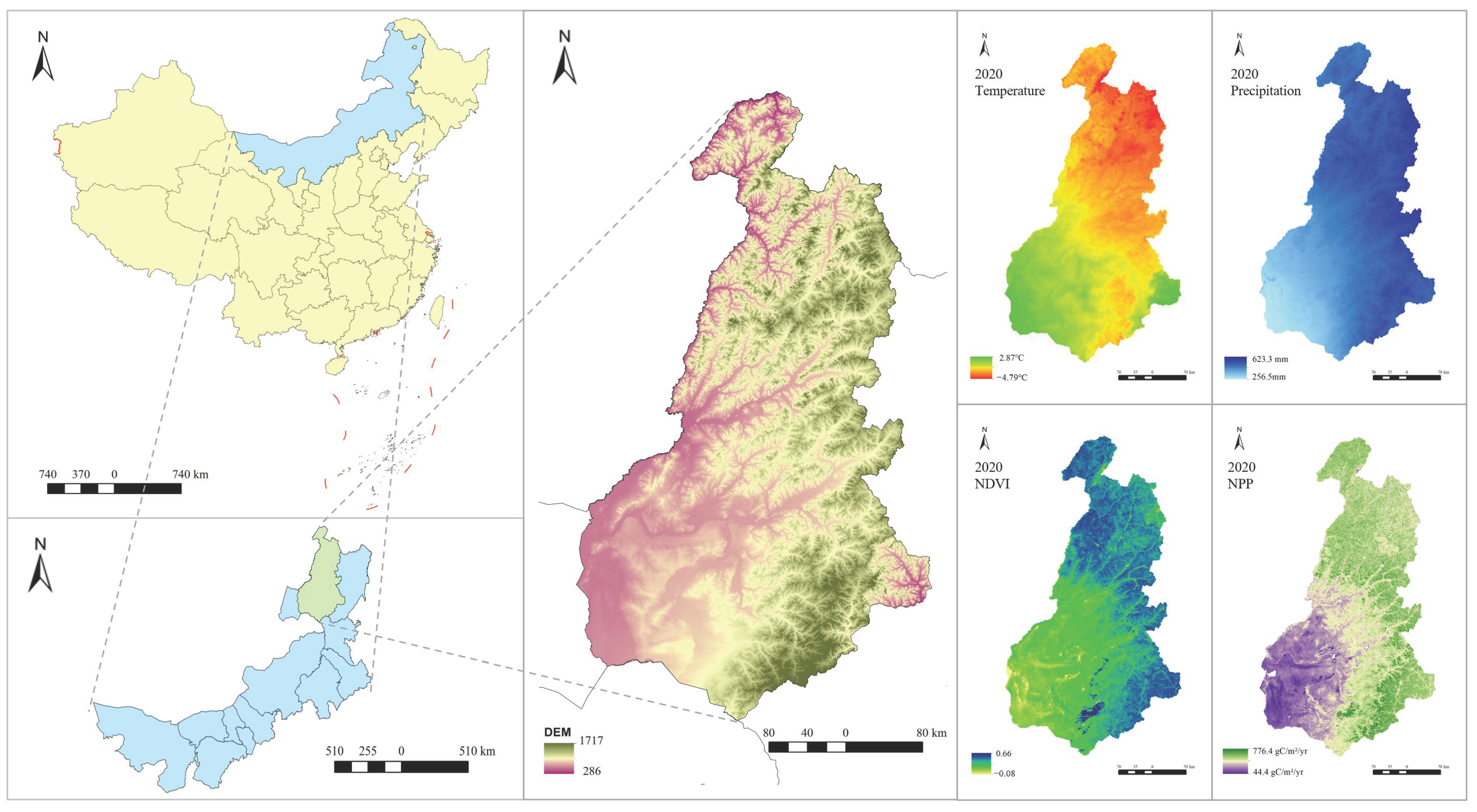
The forest–grassland ecotone of the Greater Khingan Mountains in Inner Mongolia, China (Figure 1) is not only an important ecological barrier in northern China but also an important ecologically fragile area. It is located in the central part of Hulunbuir, Northeast Inner Mongolia, covering an area of about 134,300 km2, extending about 696 km from north to south and about 384 km from east to west. The study area contains seven banners (district and county-level cities), including Xin Barag Left Banner, Ewenki Autonomous Banner, Hailar District, Prairie Chenbarhu Banner, Yakeshi City, Genhe City, and Ergun City. The terrain of the whole region is high in the east and low in the west, which belongs to the shallow mountainous, and hilly area. The region has a temperate continental monsoon climate, hot and rainy in summer, and cold and dry in winter, with an average temperature of 2.1 °C and annual precipitation of 428 mm. The vegetation in this region is dominated by forest and grassland, with a coverage rate of over 90%. The meteorological and vegetation factor maps of the study area in 1990, 2000, and 2010 are presented in the Supplementary Materials Figures S1–S3.
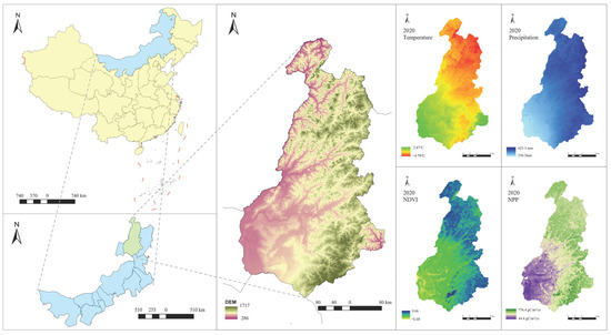
Figure 1.
The location, climate, and vegetation of the forest–grassland ecotone in the Greater Khingan Mountains, Inner Mongolia.
2.2. Data Sources and Preprocessing
The data used in this study include land cover, precipitation, temperature, night light, elevation, population density, normalized difference vegetation index (NDVI), and net primary productivity (NPP). The land-cover data were derived from the 30 m annual China land-cover dataset (CLCD) from 1985 to 2022 (https://zenodo.org/records/5816591#.ZAWM3BVBy5c, accessed on 10 October 2024). The CLCD is the first year-by-year China landcover dataset derived from Landsat, with an overall accuracy of 79.31% [56]. ArcGIS10.8 was used to reclassify the dataset into six categories: cropland, forest, grassland, water, urban, and barren. The monthly precipitation dataset, monthly temperature dataset, and yearly nighttime light dataset at the spatial resolution of 1km were obtained from the National Tibetan Plateau Scientific Data Center (http://data.tpdc.ac.cn, accessed on 10 October 2024). The annual precipitation raster data were generated by accumulating the monthly precipitation, and the annual temperature raster data were generated by averaging the 12 monthly temperatures. The elevation data were from the Geospatial Data Cloud ASTER GDEM digital elevation dataset (http://www.gscloud.cn/search, accessed on 10 October 2024). The population density data were from the Centre for Resource Environmental Science and Data (CRESD) (https://www.resdc.cn/DOI:10.12078/2017121101, accessed on 10 October 2024). Due to the lack of population density data for 2020, the data for 2019 was used to represent the population density for 2020. The NDVI data came from the Global Change Research Data Publishing and Repository (https://www.geodoi.ac.cn/edoi.aspx?DOI=10.3974/geodb.2023.04.06.V1, accessed on 10 October 2024). The NPP data were from the MODIS 17A3.006 dataset in Google Earth Engine (https://code.earthengine.google.com, accessed on 10 October 2024). The geographical coordinate system of all spatial data is WGS_1984_Albers.
2.3. Research Methods
In this study, the land use classification data of the study area during the period of 1990 to 2020 was used to analyze the transfer status of different landscape types in ArcGIS. The fishnet split method was used to divide the landscape units, and the landscape stability index was computed based on the landscape indices obtained from Fragstats 4.2. In order to explore the spatiotemporal change characteristics of landscape stability, the Kriging interpolation method was used to obtain the geospatial distribution pattern of landscape stability, and the changes in landscape stability and transfer trends were analyzed. Then, the stability ellipse model and centroid model were used to determine the spatial migration dynamics of the landscape stability in the study area. Finally, the Geodetector and Geographically Weighted Regression (GWR) models were adopted to reveal the potential driving factors and spatial distribution of dominant driving factors for the changes in landscape stability patterns.
2.3.1. Conversion of Different Landscape Types
By superimposing the maps of land classification types in different periods after reclassification, we quantitatively analyzed the transformation of each landscape type in different periods in order to reflect the dynamic trend of landscape type transfer from 1990 to 2020. The landscape transfer matrix is as follows:
where Kab refers to the area (km2) of the ath type of landscape in the initial period transformed into the bth type of landscape in the final period; n is the number of land use types.
2.3.2. Calculation of Landscape Pattern Index
Landscape stability is closely associated with landscape structure, landscape shape, and landscape heterogeneity [32,57]; thus, the following landscape indices were selected based on the three aspects: patch density (PD), landscape shape index (LSI), total edge contrast index (TECI), contagion (CONTAG), Shannon’s diversity index (SHDI), and Shannon’s evenness index (SHEI). Fragstats 4.2 was used to calculate the landscape indices of the study area. Spearman’s correlation analysis was also performed on the above indicators using SPSS 26.0 to exclude the indicators with significant correlation (Table 1). The results showed that PD was significantly correlated with LSI, CONTAG was significantly correlated with SHDI and SHEI, and SHDI and SHEI were highly correlated at the significance level of 0.01. Thus, PD, TECI, and CONTAG were selected for further landscape analysis in the study area.

Table 1.
Spearman correlation coefficients between different landscape indices.
2.3.3. Calculation of Landscape Stability and Classification
According to the theory of hierarchical patch dynamics, if the CONTAG of the landscape is higher, the PD and the TECI are smaller, the landscape stability of the landscape system will be less likely to change when confronted with disturbance [34,58]. Therefore, the landscape stability evaluation model can be constructed as follows:
where S refers to the landscape stability of each landscape unit, C refers to CONTAG, P refers to PD, and T stands for TECI. Higher values of S tend towards a steady state, and vice versa for an unstable state.
According to the principle that the landscape sample area should be 2–5 times the average patch area in order to better reflect the pattern information of the surrounding landscape in the sampling area [59,60], this study used the fishnet tool in ArcGIS 10.8 software to set up the fishing grid at the grid size of 15 km × 15 km and divide the study area into 690 regular grid units (Supplementary Materials: Figure S4). Based on the landscape indices obtained from Fragstats 4.2, the landscape stability value in each grid unit was calculated using the landscape stability evaluation model, and the fishing grid was connected to the landscape stability value in the grid unit. The Kriging interpolation method and the normalization method were adopted to obtain the landscape stability of the whole study area [61]. In order to achieve a balance between highlighting the changes in landscape stability intermediate values and extreme values while maximizing the category differences as much as possible, the landscape stability was divided into five levels: unstable, less stable, relatively stable, stable, and extremely stable, based on the geometrical interval method [62], the natural breakpoint method [32], and the data distribution of each grid unit by year.
2.3.4. Analysis of Spatial Migration of Landscape Stability Pattern
The centroid model and standard deviation ellipse model are commonly used statistical methods for revealing the spatial distribution characteristics of geographic elements [63,64]. This study merged the stable and extremely stable landscape areas in ArcGIS 10.8 and introduced the standard deviation ellipse and stability centroid migration model to analyze the spatial migration trend of landscape stability in the forest–grassland ecotone of the Greater Khingan Mountains, Inner Mongolia based on the relative position of the centroid migration as well as the parameters of the major and minor axes of the standard deviation ellipse. The centroid model is expressed in Equation (3), and the standard deviation ellipse model is expressed in Equations (4)–(9).
where M(SDEx, SDEy) is the landscape stability centroid of the study area, xi and yi are the geographical coordinates of each element, X and Y are the arithmetic mean centers, θ is the inclination angle of the ellipse (x-axis based, north direction as 0 degree, and rotates clockwise), and are the differences between the mean center and the xy coordinates; σx is the length of the x-axis of the ellipse; σy is the length of the y-axis of the ellipse; n is the number of units.
2.3.5. Analysis of Driving Factors of Landscape Stability Pattern
According to the core principle of GeoDetector 1.0-3, if an independent variable has a significant impact on a dependent variable, then the spatial distribution of the independent and dependent variables should be similar [65]. In this study, the GeoDetector was used to analyze the driving mechanism of landscape stability in the study area from 1990 to 2020. The following driving factors from four categories were taken into consideration: meteorological driving factors (temperature and precipitation), vegetation driving factors (NPP and NDVI), policy driving factors (Natural Forest Protection Program), and social driving factors (population and nighttime light). The study mainly focused on two modules (factor detection and interaction detection) in order to reveal the driving mechanism of different driving factors on the spatial differentiation of landscape stability in the forest–grassland ecotone of the Greater Khingan Mountains, Inner Mongolia.
Factor detection refers to the extent to which the driving factor X can explain the spatial differentiation of attribute Y, which is measured by the q value, the specific calculation formula is as follows:
where h = 1, …, L represents the stratification of variable Y or factor X; Nh and N are the number of units in stratum h and the whole area, respectively; σ2h and σ2 are the variances of Y values in stratum h and the whole area, respectively. SSW and SST are the sum of variances within the layer (Within Sum of Squares) and the total variance of the entire region (Total Sum of Squares). The range of q value is [0, 1]. The larger the q value, the stronger the explanatory power of the driving factor.
Interaction detection is used to evaluate the interaction between different driving factors Xs. In other words, it is to evaluate whether the joint effect of driving factors X1 and X2 will increase or weaken the explanatory power of the dependent variable Y, or whether the impact of these driving factors on Y is independent of each other. The interrelationships between driving factors are shown in Table 2.
Table 2.
Relationships between driving factors in interaction detection.
2.3.6. Spatial Heterogeneity of Dominant Driving Factors
Geographically Weighted Regression (GWR) is a spatial statistical technique that models the relationship between a dependent variable and independent variables while allowing for spatial variation in the model parameters, making it sensitive to local geographic variations. In this study, the GWR model was used to explore the mechanism of the dominant driving factors on the pattern of landscape stability at the spatial level. The GWR model is expressed as follows:
where yi is the landscape stability value of sample i, (ui,vi) are the spatial geographical coordinates of sample i, ρ0 (u0,v0) is the estimated constant value of the sample point, ρj (uj,vj) is the jth regression coefficient of sample point i, xij is the value of the jth independent variable in sample point i, and εi is a normal distribution error with a mean value of 0.
In this study, the 15 km × 15 km grids were used to mesh the dominant driving factors and connected with the grid cells of landscape stability values. After conducting GWR analysis on the grid cells, the Kriging interpolation and the normalization method were used to explore the spatial distribution heterogeneity of the impacts of the dominant driving factors in the study area at different times. The positive values indicate positive impact and negative values indicate negative impact. The closer the coefficient is to 1, the stronger the positive impact between the two variables. The closer it is to 0, the less closely impacted the two variables are. The closer it is to −1, the stronger the negative impact between the two variables.
3. Results
3.1. Landscape Type Transformation in the Study Area from 1990 to 2020
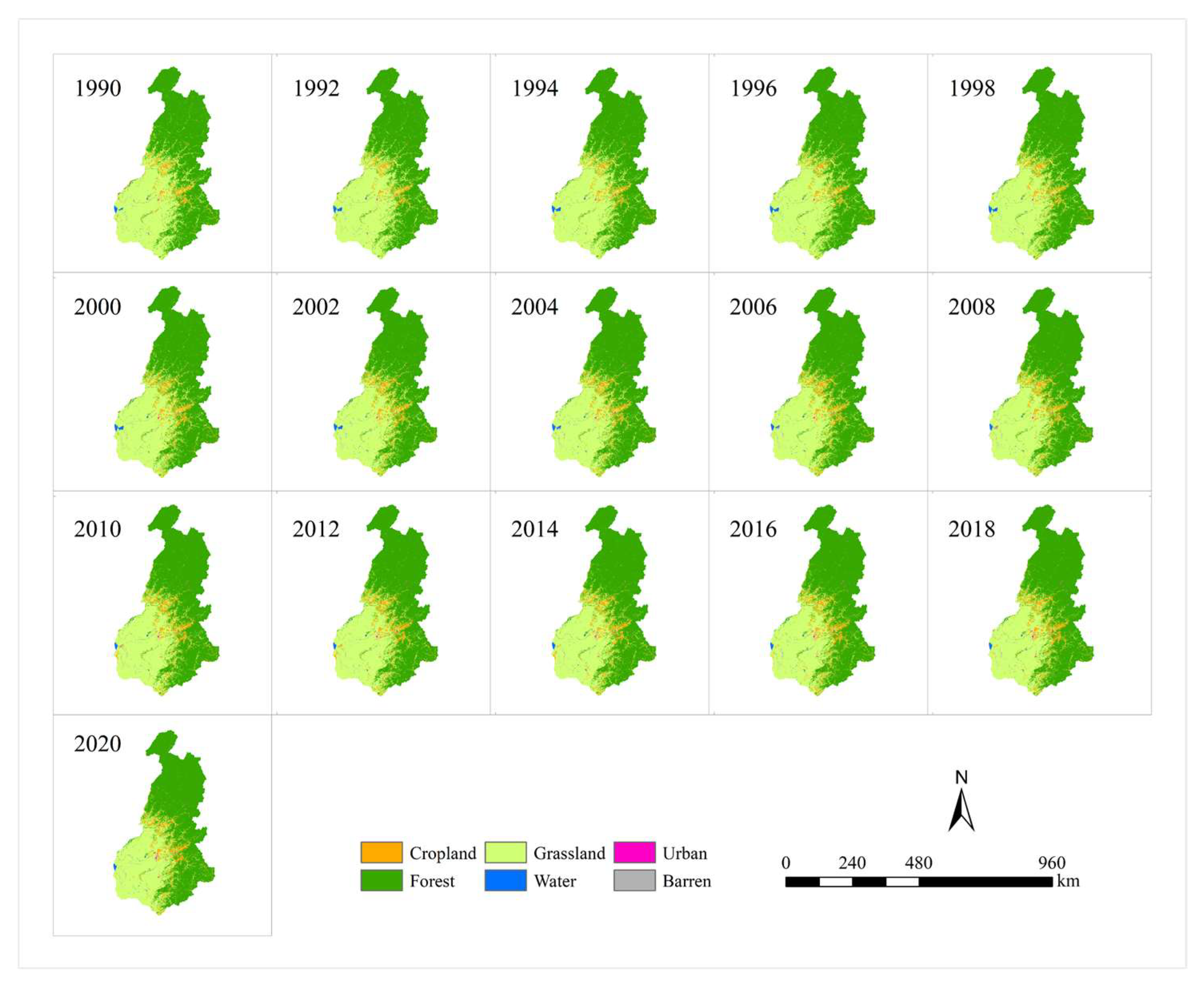
The changes in landscape types in the forest–grassland ecotone of the Greater Khingan Mountains in Inner Mongolia from 1990 to 2020 are shown in Figure 2. It can be seen that the dominant landscape types in the region have undergone certain changes within the 30 years. The proportion of forest landscape coverage increased from 54.92% to 58.63%, and the proportion of grassland landscape coverage decreased from 41.03% to 35.85%. The trend of forest-dominated landscape in the forest–grassland ecotone in the Greater Khingan Mountains of Inner Mongolia has been strengthening from 1990 to 2020.
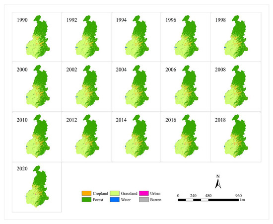
Figure 2.
Annual landscape distribution of the forest–grassland ecotone in the Greater Khingan Mountain, Inner Mongolia from 1990 to 2020.
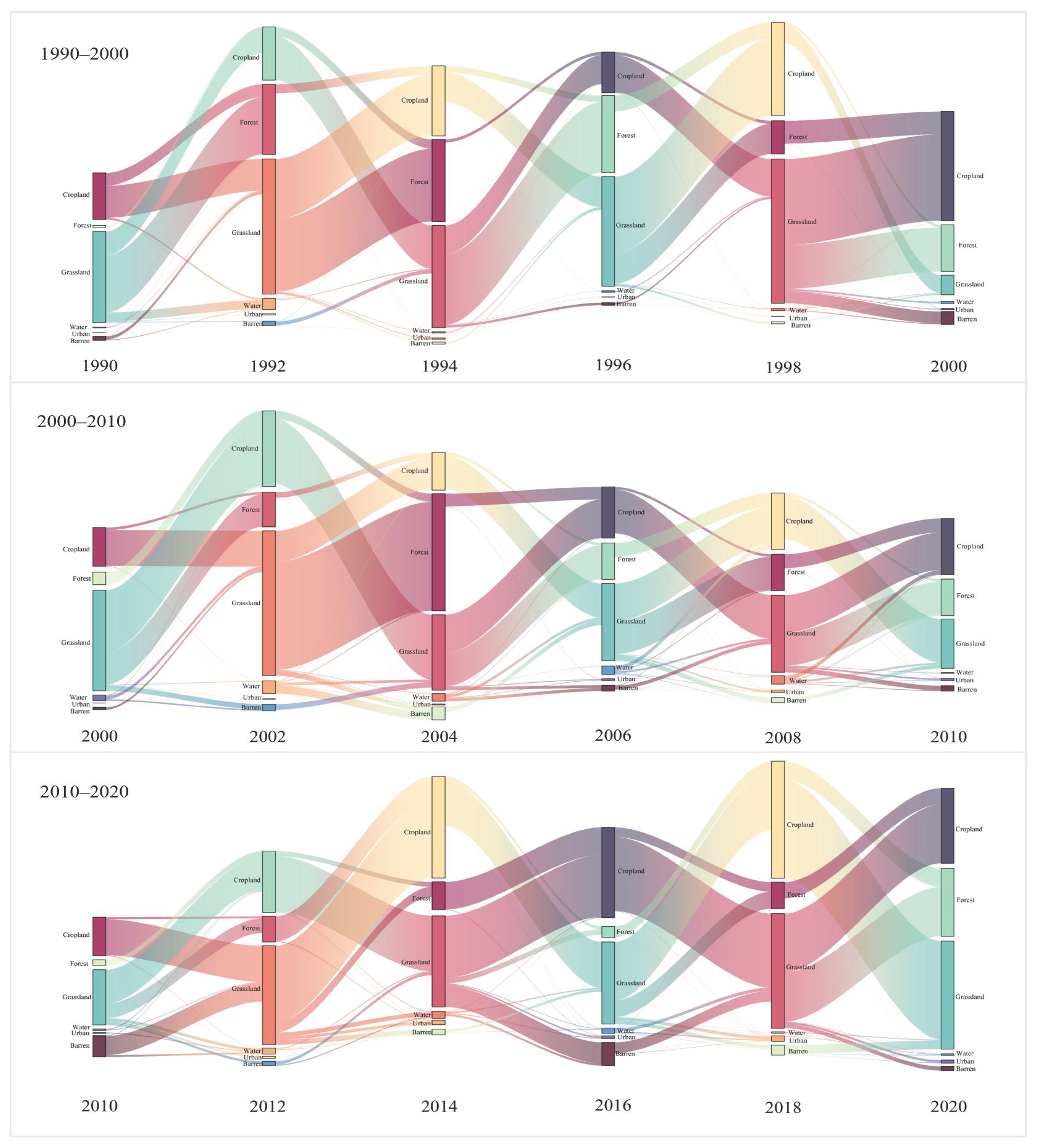
Figure 3 illustrates the dynamic trends of landscape type transfer from 1990 to 2020 (excluding non-transferred landscapes), where the left-side column represents landscape inflow (other types of landscapes are transformed into the current landscape) and the right-side column represents landscape outflow (the current landscape is transformed into other types of landscapes). As shown in Figure 3, the largest amount of land transferred out was grassland in the study area, with a total area of 8594.24 km2 transferred out in 30 years, which indicates that grassland had shown a certain degradation trend. Of which, 5218.52 km2 of grassland was converted into forests. This may be due to the fact that grassland was gradually replaced by shrubs and trees after natural succession due to climate change and human disturbance in areas where forest–grassland ecosystems were intertwined. In total, 2994.08 km2 of grassland was converted into cropland, 140.28 km2 was converted into an urban area, and 191.13 km2 of grassland was converted into barren, due to the impacts of increasing social demand, overgrazing, over-reclamation, and natural disasters (e.g., grassland fires, flooding). The largest amount of transfer was in forests, mainly from cropland and grassland with a cumulative area of 5732.3 km2, followed by cropland with a cumulative area of 1505.6 km2. In addition, the urban area also increased steadily, with a cumulative increase of 210.3 km2, while the areas of water and barren all showed a downward trend.
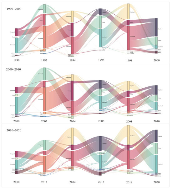
Figure 3.
Dynamic trends of landscape type transfer from 1990 to 2020 (excluding non-transferred landscapes).
3.2. Dynamic Characteristics of Landscape Index in the Forest–Grassland Ecotone of the Greater Khingan Mountains in Inner Mongolia
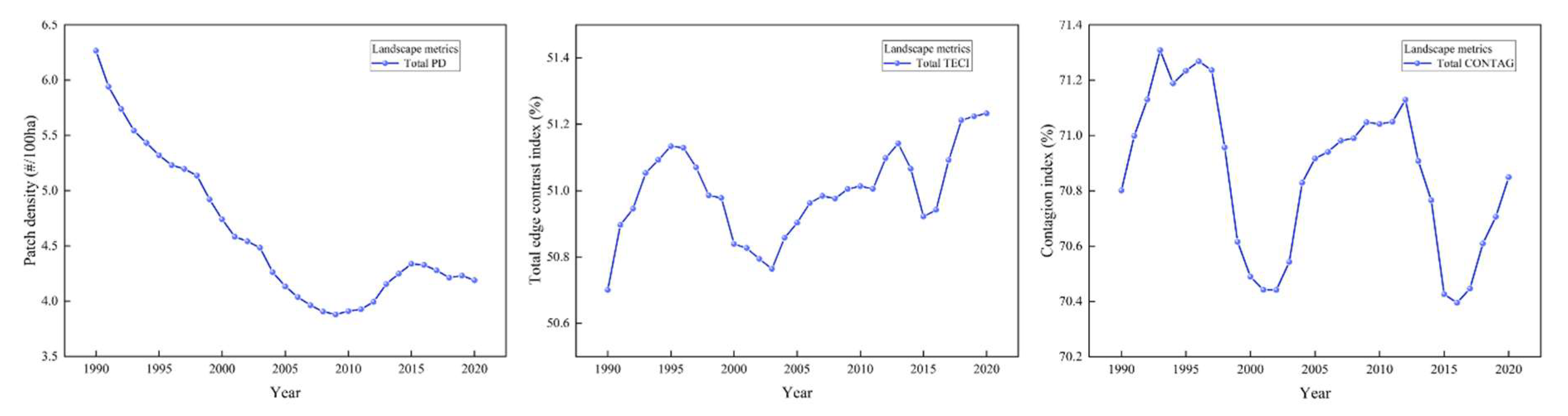
The dynamic changes in landscape indices and stability in the study area are shown in Figure 4. The overall PD value of the forest–grassland ecotone in the study area basically showed a decreasing trend, which indicates that the overall patch density gradually decreased, larger patches tended to dominate the landscape, and the degree of landscape fragmentation decreased relatively. By studying the PD index of various types of landscapes in the study area, the results showed that grassland landscapes had the highest PD, followed by forest landscapes, and urban and water landscapes had the lowest patch density. TECL showed a trend of first increasing, then decreasing and then increasing again over time. The increasing trend was observed in 1990–1995, 2003–2012, and 2016–2020, respectively. This may be due to the fact that human activities such as urban expansion increased the contrast degree between habitat edges and other landscape types. Among different landscapes in the study area, the urban landscape had the highest TECL, followed by the water landscape, and the cropland landscape had the lowest TECL. The landscape index CONTAG ranged from 70.4% to 71.4%, which was slightly fluctuating but relatively stable, indicating that the overall landscape configuration in the study area was relatively stable and patches were relatively concentrated in space.
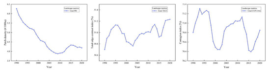
Figure 4.
Dynamic changes in landscape indices and stability of the forest–grassland ecotone in the Greater Khingan Mountain, Inner Mongolia from 1990 to 2020.
3.3. Spatial Pattern Changes and Transfer Characteristics of Landscape Stability in the Forest–Grassland Ecotone of the Greater Khingan Mountains in Inner Mongolia
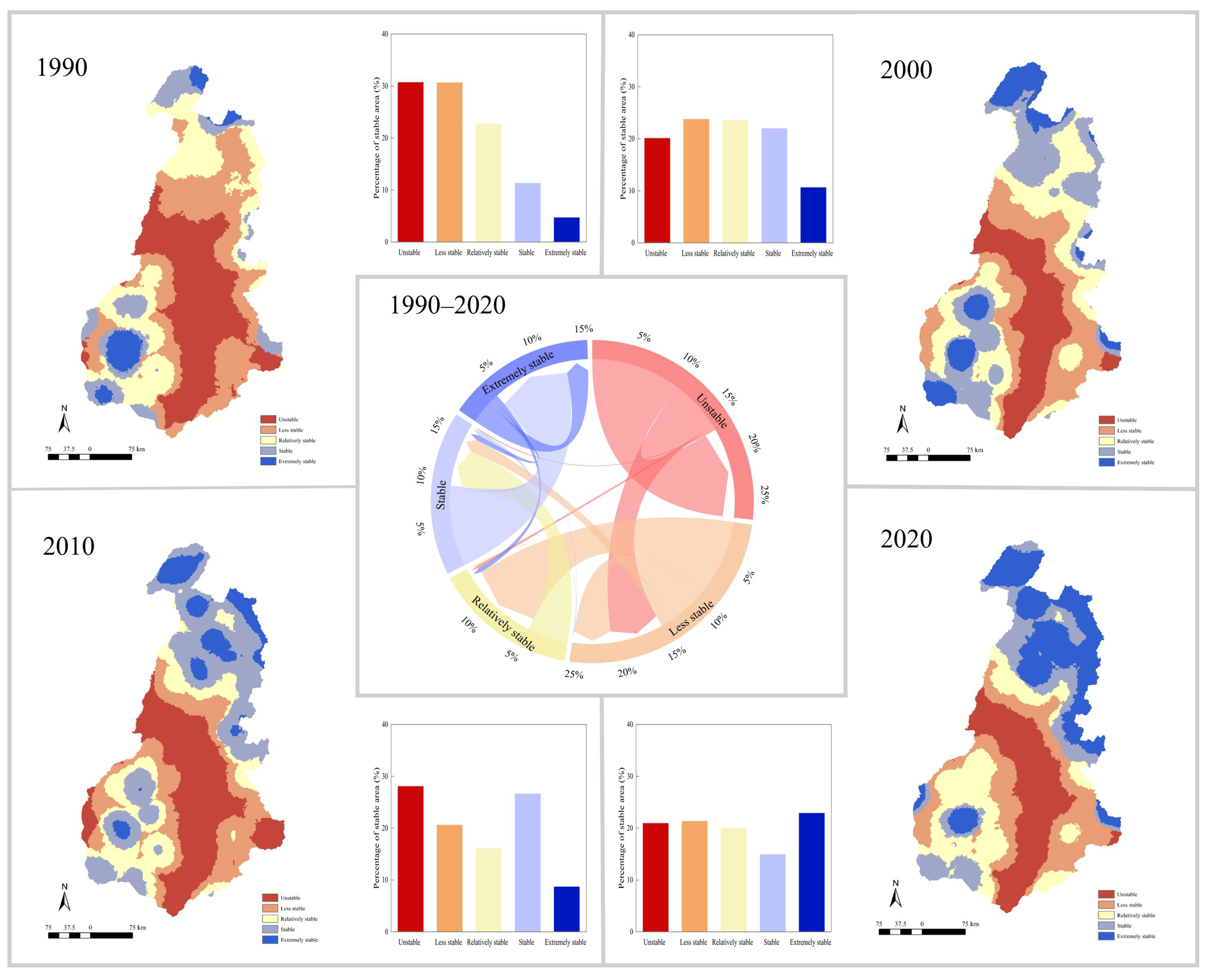
Figure 5 shows the changes in the spatial pattern of landscape stability in the forest–grassland ecotone of the Greater Khingan Mountains in Inner Mongolia from 1990 to 2020. Overall, the landscape stability showed an improving trend over time. The landscape in 1990 was dominated by unstable and less stable areas, with a total area of about 82,263.68 km2, accounting for about 61.31%, while stable and extremely stable areas accounted for about 15.96%. From 1990 to 2000, the proportion of unstable areas decreased significantly, and the proportion of stable areas increased significantly. By 2010, the proportion of unstable and less stable landscape areas decreased to 48.63%, and the proportion of stable and extremely stable areas was about 35.28%, an increase of 19.32% over 1990. By 2020, the extremely stable landscape area had increased significantly, reaching about 30,695.83 km2, accounting for about 22.88% of the total area.

Figure 5.
Changes in the spatial pattern of landscape stability of the forest–grassland ecotone in the Greater Khingan Mountains, Inner Mongolia from 1990 to 2020.
The variations in landscape stability classification in the study area are shown in the center of Figure 5. It is found that the study area was mainly characterized by the transfer-out of the unstable class and the transfer-in of the stable class during the period of 1990 to 2020. The area from unstable to less stable level was about 16,168.2 km2, the area from less stable to relatively stable level was about 23,645.84 km2, the area from relatively stable to stable level was about 12,183.93 km2, and the area from stable to extremely stable level was about 23,592 km2. In sum, each landscape stability class basically showed a trend of transformation from a low-stability level to a higher-stability level.
3.4. Migration Trends of the Spatial Pattern of Landscape Stability in the Forest–Grassland Ecotone of the Greater Khingan Mountains in Inner Mongolia
The landscape stability area of the forest–grassland ecotone in the study area extended year by year in the northeast-southwest direction (Figure 6). The area of stable landscape increased from 21,451.2 km2 to 50,071.1 km2, and the spatial migration of the stable area also led to the shift in the centroid and the standard deviation ellipse of landscape stability in the study area. As shown in Figure 6, the center of landscape stability in the study area basically showed a trend of shifting from southwest to northeast. Within the 30 years, the stability center of the study area moved from 119°43′ E to 120°43′ E, and from 49°36′ N to 50°35′ N, with a shifting distance of about 132.4 km. It is worth noting that the stability center in 2000–2005 shifted from northeast to southwest, which was due to the significant increase in the stable landscape area in the central part in 2000–2005, resulting in the migration of the landscape stability center to the southwest.
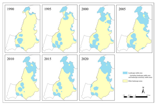
Figure 6.
Understory spatial migration of the stable landscape area in the forest–grassland ecotone of the Greater Khingan Mountains in Inner Mongolia from 1990 to 2020.
The standard deviation ellipse of landscape stability in the study area also shifted to a certain extent within 30 years (Figure 7). The long axis of the stability ellipse decreased from 281.15 km in 1990 to 253.29 km in 2020, and the short axis increased from 92.53 km in 1990 to 110.02 km in 2020. This indicates that the stable landscape in the study area was more closely distributed in the northeast-southwest direction, showing increased landscape stability, while the stability was extended and diffused in the southeast–northwest direction. In addition, the ratio of the short axis to the long axis of the stability ellipse had certain fluctuations between 1990 and 2020, which indicates that the expansion speed of the region in the north–south direction and in the east–west direction was not stable.
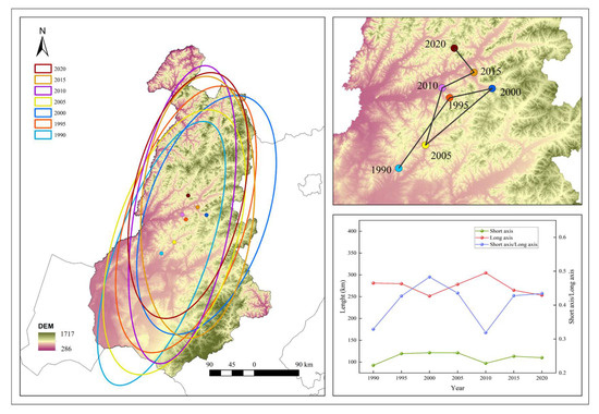
Figure 7.
Dynamic changes in landscape stability centroid and standardized deviation ellipse in the forest–grassland ecotone of the Greater Khingan Mountains in Inner Mongolia.
3.5. Analysis of Driving Factors for Landscape Stability in the Forest–Grassland Ecotone of the Greater Khingan Mountains in Inner Mongolia
Results showed that the influences of different factors (i.e., temperature, precipitation, NPP, NDVI, forest area, population, and nighttime light) on the landscape stability of the forest–grassland ecotone in the study area changed over time. As shown in Table 3, climate factors (temperature and precipitation) were the dominant factors affecting the landscape stability pattern in the study area. The explanatory power (q value) of temperature increased from 0.297 in 1990 to 0.478 in 2020. The q value of precipitation increased from 0.349 in 1990 to 0.505 in 2010. Although the q value of precipitation decreased to 0.208 in 2020, the explanatory power of this factor was still higher than that of most other types of influencing factors. Therefore, the climate factors had significant driving effects on the landscape stability of the forest–grassland ecotone in the study area. Vegetation factors (including NPP and NDVI) all also showed a significant relationship with the landscape stability in the study area, but the driving force intensity was lower than that of climate driving factors, thus they were secondary driving factors. In addition, with the implementation of the National Natural Forest Protection Program, the impact of forest area on landscape ecological stability increased from 0.55% in 1990 to 8.64% in 2020. Both population and nighttime lighting factors had relatively little impact on the landscape stability and the impact of population changed from significant to insignificant. This may be because the population density in the study area was low and decreased over the years, so the impacts of human activities on the overall landscape stability became insignificant.
Table 3.
q values of different driving factors for landscape stability.
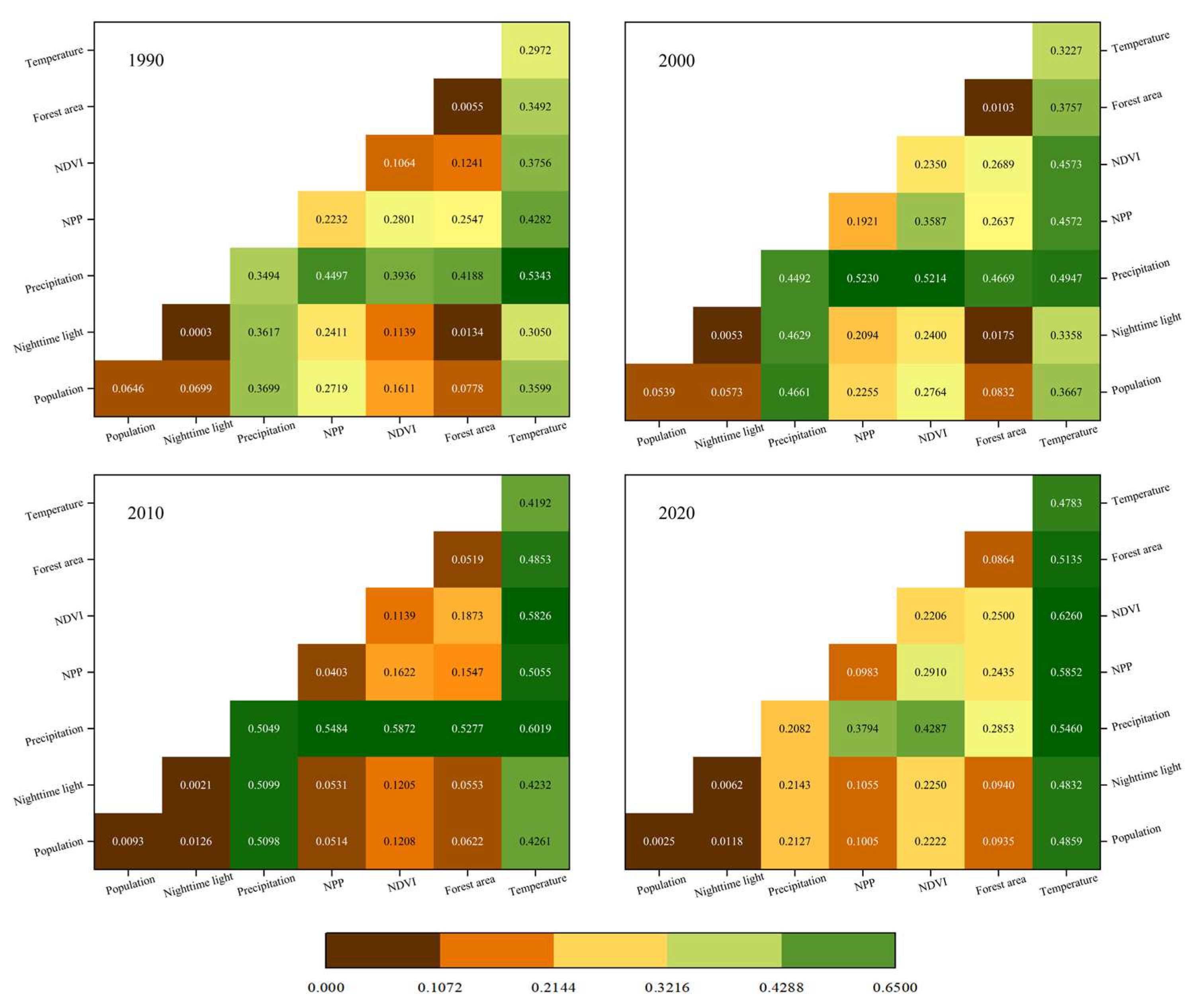
Since landscape stability is simultaneously affected by multiple factors, which are also mutually affected, the interaction detector was used to further explore the impacts of the interactions of different factors on the spatial differentiation of landscape ecological stability in the forest–grassland ecotone of the study area. The interaction test results showed two effects: bivariate enhancement and nonlinear enhancement (Figure 8). Different combinations of climate-driving factors and vegetation-driving factors showed good interactive effects. For example, the interaction between precipitation and NPP in 2000 can explain 52.30% of the total impact on landscape stability. Similarly, the interaction between temperature and NDVI in 2020 can explain 62.60% of the total impact on landscape stability. Therefore, the interaction effects of all driving factors on landscape stability were greater than those of the individual driving factors. The key interactions included Temperature Ո Precipitation, NPP Ո Precipitation, Temperature Ո NDVI, etc. In sum, the landscape stability in the study area was affected by bivariate and nonlinear-enhanced manners, which showed more significant effects than individual driving factors.
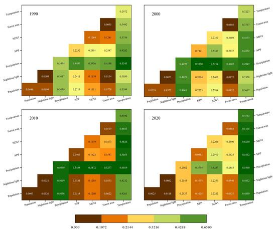
Figure 8.
Interactive effects of the driving factors on the landscape stability.
3.6. Spatial Heterogeneity of Key Driving Factors in the Forest–Grassland Ecotone of the Greater Khingan Mountains in Inner Mongolia
Based on the q value and significance in Table 3, temperature, precipitation, and NDVI were determined as the dominant factors affecting landscape stability in the study area. It was verified that the joint F values of the dominant factors all passed the significance test at the significance level of 0.001, and the variance inflation factor (VIF) test showed that the VIF values were all less than 7.5 (Supplementary Materials: Table S1), which indicates that there was no multicollinearity between the dominant factors, and GWR analysis can be further performed to determine the spatial heterogeneity of the dominant driving factors.
The average R2 of the GWR models in the study area at different time periods was 0.677, and the average adjusted R2 was 0.676 (n = 690), showing a better goodness of fit. Figure 9 illustrates the results of the GWR analysis, which shows that the dominant driving factors exhibited different spatial heterogeneity in the study area with the change in time. During the period of 1990 to 2020, the impact of temperature on landscape stability became increasingly significant, and the area with positive correlation gradually expanded. This may be influenced by global warming, with more organisms gradually showing temperature adaptability, thereby gradually enhancing the positive impact on landscape stability. In addition, the positively correlated impact area gradually spread northward over time, which may indicate that some organisms showed a northward migration trend as the global temperature rose, thereby promoting landscape stability. The driving factor of precipitation was found to have a strong positive impact on the landscape stability in the northern part of the study area and a strong negative impact in the southern part of the study area. This may be because the forest–grassland ecotone in the northern part was dominated by forests, and the increase in precipitation was more likely to promote forest growth, thereby promoting the stability of the landscape. The forest–grassland ecotone in the southern part of the study area was dominated by grasslands, and excessive increase in precipitation may cause grassland erosion, which was not conducive to landscape stability. It is noted that the spatial impact of precipitation on landscape stability in the study area in 1990 was slightly different from that in other years, probably due to the changes in the spatial distribution patterns of precipitation. In 1990–2000, NDVI showed a strong positive correlation with landscape stability in the northern part of the study area, indicating that vegetation growth promoted landscape stability. In the south, however, there was a negative correlation or a weaker impact during the period. This may be due to the fact that the grassland-dominated landscape had a weaker ability to adapt to the environment and may be more susceptible to environmental disturbances and fragmentation, which was not conducive to the stability of the overall landscape. As time went by, NDVI in the southern part of the study area showed a positive correlation trend with landscape stability, which may be affected by the expansion of forests in the forest–grassland ecotone.
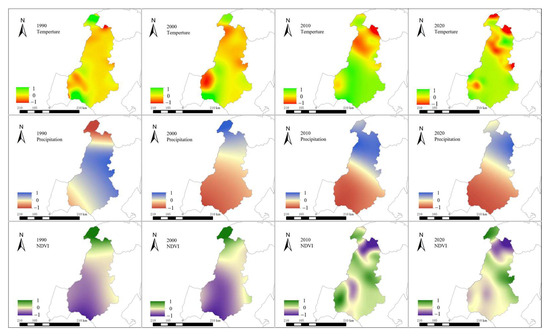
Figure 9.
Spatial heterogeneity of key driving factors in the forest–grassland ecotone of the Greater Khingan Mountains in Inner Mongolia from 1990 to 2020.
4. Discussion
4.1. Changes in Landscape Stability Pattern in the Forest–Grassland Ecotone of the Greater Khingan Mountains in Inner Mongolia from 1990 to 2020
Landscape pattern is a key factor affecting the balance and health of ecosystems [66]. A stable landscape pattern can promote interactions between species, enhance the resilience of ecosystems, and thus increase the resilience of ecosystems [67,68]. Our study evaluated the landscape stability of the forest–grassland ecotone in the Greater Khingan Range, Inner Mongolia. The results showed that from 1990 to 2020, the landscape stability of the study area gradually improved. The landscape stability level basically showed a trend of transformation from a low-stability level to a higher-stability level. Guo et al. [3] analyzed the landscape fragmentation of forest–grassland ecotone in northern China from 1990 to 2020 and found that the proportion of highly fragmented areas decreased by more than 10% within 30 years, while the proportion of moderately and lowly fragmented areas increased. This indirectly indicates that the landscape in the forest–grassland ecotone was gradually becoming more stable over time. By comparing the stability of arid oases [69], karst mountain cities [32], wetlands [70,71], and lakes [72], we found that landscape stability in most areas was not ideal over time, and some areas with improved landscapes may be greatly affected by policy interventions. Compared with single ecosystems such as wetlands, watersheds, and mountains, the forest–grassland ecosystem provides higher biodiversity, has stronger self-regulation ability and self-adaptation function, and exhibits stronger landscape stability. Our study found that the forest–grassland ecotones in the study area were more significantly affected by climate factors, while other areas, such as watersheds, may be more susceptible to human disturbance which is more sudden than natural disturbances. This suggests that interlaced ecosystems may show better landscape variation trends than single ecosystems, and the unique ecological advantages of forest–grassland ecotones cannot be ignored.
4.2. Spatial Migration Trend of Landscape Stability in the Forest–Grassland Ecotone of the Greater Khingan Mountains in Inner Mongolia from 1990 to 2020
Standard deviation ellipse and centroid migration can accurately reveal the spatial distribution characteristics of geographic units. Current landscape studies mainly focus on risk centers and risk ellipses to study regional landscape migration [73,74,75,76]. Our study is the first to introduce landscape stability centers and landscape stability ellipses by combining stable and extremely stable landscapes in landscape research. The study showed that the landscape stability of the forest–grassland ecotones in the study area was basically extended in the direction of southwest to northeast. From the maps of landscape stability change in the study area (Figure 5 and Figure 6), the landscape stability pattern showed a gradual stabilization from the middle to the northeast and southwest edges from 1990 to 2020, showing a stability transition trend of southwest-northeast belt spreading. The stability center basically showed a shift from southwest to northeast, which was due to the degrading of the grassland in the southwest area and forest encroachment into grasslands in the northeast area. A study published in the Journal of Science [77] showed that the world’s fauna and plants were migrating further to northern and alpine regions due to climate change, and the forest–grassland ecotone with rich species diversity in this study reflected a similar trend.
4.3. Analysis of Driving Factors of Landscape Stability in the Forest–Grassland Ecotone of the Greater Khingan Mountains in Inner Mongolia from 1990 to 2020
According to the Synthesis Report for the Sixth Assessment Report of the Intergovernmental Panel on Climate Change, the global surface temperature has increased by 1.1 °C compared to the c level, and human activities have also affected global precipitation [78]. It is noted that the average temperature in the study area increased by 0.64 °C and the precipitation decreased by 79.2 mm from 1990 to 2020. Our results indicated that climate factors (temperature and precipitation) were the main factors affecting the stability of the landscape pattern in the study area during the period from 1990 to 2020. The impact also increased over time, indicating that the forest–grassland ecotone was being affected by climate change [1]. This climate change had a direct impact on ecosystems and drove changes in landscape stability in the study area. Vegetation factors (including NPP and NDVI) were indirectly affected by climate, but the driving force intensity in the study area was lower than that of climate factors. In addition, with the implementation of China’s Natural Forest Protection Project [79,80], the impact of forest area on landscape ecological stability gradually increased, which maintained the regional ecological stability to a certain extent and promoted the stable balance of the landscape. Human disturbances are believed to have great impacts on the landscape fragmentation of forest–grassland ecotones [3]; however, our study found that human factors (including population and light) did not significantly affect the landscape stability of the forest–grassland ecotone. It should be noted that some policy factors (e.g., banning grazing and resting grazing on grassland) cannot be quantified spatially, which were not considered in the anthropogenic disturbance factors. In addition, different research perspectives also contribute to the differences in the impacts of different driving factors on the landscape of the forest–grassland ecotone. Therefore, the effects of human interference still need to be further explored when relevant data are available.
Forest expansion can reduce forest fragmentation and improve ecosystem stability in fragile landscapes [81]. The study further analyzed the spatial heterogeneity of the dominant factors through GWR. The results showed that precipitation and NDVI were positively correlated with landscape stability in the northern region of the study area. Since the dominant landscape in this part was forest, precipitation was conducive to the growth of forests and thus promoted the stability of the landscape. Zhai et al. [82] analyzed the meteorological factors on forest growth rate in the southeast slope of Taihang Mountains, China, and found that forest growth stock could increase by 21.1 m3∙hm−2 when precipitation increases by 100 mm. Babst et al. [83] indicated that climate change had positive impacts on forest growth in cold-humid environments. However, precipitation and NDVI were found to have negative impacts on the landscape stability of the south grassland-dominated forest–grassland ecotone. Compared to forests, grasslands were more susceptible to precipitation erosion and external disturbance [84]. Even if the NDVI of grassland increased, fragmentation was still likely to occur. In addition, as time went by, the area positively correlated with temperature and NDVI gradually expanded in the south, which indicated that the grassland-dominated area gradually adapted to the changes in temperature and NDVI, and the area positively correlated with landscape stability gradually expanded.
4.4. Limitations and Future Research
The edge effect of the double-superimposed ecosystem brings both fragility and stability to the forest–grassland ecotone. Previous studies on this area mainly focused on risk assessment. Although this study systematically discussed the issue from the perspective of landscape stability, the research scale is based on macro landscape stability, which may ignore the details of landscape stability changes in some regions. In the future, more detailed information and data acquisition methods (e.g., Unmanned Aerial Vehicle, LIDAR) can be combined to carry out multi-scale information fusion to further study the landscape pattern of forest–grassland ecotones.
5. Conclusions
A comprehensive evaluation of the changes in the health and stability of the forest–grassland ecotone is of great significance for ecological monitoring and restoration in the region. The study conducted dynamic monitoring and driving force analysis on the landscape stability in the forest–grassland ecotone of the Greater Khingan Mountains in Inner Mongolia, China from 1990 to 2020. The results showed that the landscape pattern of the forest–grassland ecotone in the study area had changed over time and the overall situation of landscape stability was gradually improving. The spatial pattern of landscape stability showed a southwest-northeast belt-like spreading, and the stability center gradually migrated to the northeast. In addition, the study found that climate factors were the main driving factors affecting landscape stability changes, human factors did not have a significant impact on landscape stability, and different dominant driving factors showed different spatial heterogeneity over time. This study explored the unique ecological advantages of the forest–grassland ecotone from the perspective of landscape stability changes, which will help ecological restoration departments to further conduct ecological assessments of the forest–grassland ecotone, and may also provide references for the ecological landscape research in other forest–grassland ecotone areas.
Supplementary Materials
The following supporting information can be downloaded at https://www.mdpi.com/article/10.3390/land14020396/s1, Figure S1. Meteorological and vegetation factor maps of the study area in 1990. Figure S2. Mete-orological and vegetation factor maps of the study area in 2000. Figure S3. Meteorological and vegetation factor maps of the study area in 2010. Figure S4. The study area for fishery grid division. And Table S1. OLS table for selecting the leading driving factors.
Author Contributions
Conceptualization, Q.H. and J.W.; methodology, Q.H., J.W. and W.L.; software, Q.H.; validation, Q.H., J.W. and W.L.; formal analysis, Q.H.; investigation, Q.H.; writing—original draft preparation, Q.H. and J.W.; writing—review and editing, J.W. and W.L.; supervision, J.W. and W.L.; project administration, J.W.; funding acquisition, J.W. All authors have read and agreed to the published version of the manuscript.
Funding
This research was funded by the National Key R&D Program of China (2023YFF1304001-03).
Institutional Review Board Statement
Not applicable.
Informed Consent Statement
Informed consent was obtained from all participants involved in the study.
Data Availability Statement
The data used to support the findings of this study are available from the corresponding author upon request.
Conflicts of Interest
The authors declare no conflicts of interest.
References
- Myster, R.W. Ecotones Between Forest and Grassland; Springer: New York, NY, USA, 2012. [Google Scholar]
- You, G.Y.; Liu, B.; Zou, C.X.; Li, H.D.; McKenzie, S.; He, Y.Q.; Gao, J.X.; Jia, X.R.; Arain, M.A.; Wang, S.S.; et al. Sensitivity of vegetation dynamics to climate variability in a forest-steppe transition ecozone, north-eastern Inner Mongolia, China. Ecol. Indic. 2021, 120, 106833. [Google Scholar] [CrossRef]
- Guo, J.; Li, Y.H.; Ma, W.; Guo, Q.H.; Cheng, K.; Ma, J.; Wang, Z.W. Changes of Chinese forest-grassland ecotone in geographical scope and landscape structure from 1990 to 2020. Ecography 2024, 2024, e07296. [Google Scholar] [CrossRef]
- Manning, A.D.; Gibbons, P.; Lindenmayer, D.B. Scattered trees: A complementary strategy for facilitating adaptive responses to climate change in modified landscapes? J. Appl. Ecol. 2009, 46, 915–919. [Google Scholar] [CrossRef]
- Tian, C.; Yang, X.B.; Liu, Y. Edge effect and its impacts on forest ecosystem: A review. Chin. J. Appl. Ecol. 2011, 22, 2184–2192. [Google Scholar]
- Banerjee, S.; Thrall, P.H.; Bissett, A.; Heijden, M.G.A.; Richardson, A.E. Linking microbial co-occurrences to soil ecological processes across a woodland-grassland ecotone. Ecol. Evol. 2018, 8, 8217–8230. [Google Scholar] [CrossRef]
- Lashchinskiy, N.; Korolyuk, A.; Makunina, N.; Anenkhonov, O.; Liu, H.Y. Longitudinal changes in species composition of forests and grasslands across the North Asian forest steppe zone. Folia. Geobot. 2017, 52, 175–197. [Google Scholar] [CrossRef]
- Morgan, P.; Heyerdahl, E.K.; Strand, E.K.; Bunting, S.C.; Riser, J.P.; Abatzoglou, J.T.; Nielsen-Pincus, M.; Johnson, M. Fire and land cover change in the Palouse Prairie-forest ecotone, Washington and Idaho, USA. Fire Ecol. 2020, 16, 2. [Google Scholar] [CrossRef]
- Shumilovskikh, L.; Sannikov, P.; Efimik, E.; Shestakov, I.; Mingalev, V.V. Long-term ecology and conservation of the Kungur forest-steppe (pre-Urals, Russia): Case study Spasskaya Gora. Biodivers. Conserv. 2021, 30, 4061–4087. [Google Scholar] [CrossRef]
- Liu, L.C.; Lu, X.S.; Lv, S.H.; Lin, D. Analysis of landscape sustainability in Hulunbeir Forest-Steppe ecotone. Pratacult. Sci. 2008, 25, 119–124. [Google Scholar]
- Li, S.J.; Sun, Z.G.; Tan, M.H.; Guo, L.L.; Zhang, X.B. Changing patterns in farming-pastoral ecotones in China between 1990 and 2010. Ecol. Indic. 2018, 89, 110–117. [Google Scholar] [CrossRef]
- Hou, W.; Walz, U. Enhanced analysis of landscape structure: Inclusion of transition zones and small-scale landscape elements. Ecol. Indic. 2013, 31, 15–24. [Google Scholar] [CrossRef]
- Qiao, Z.; Yang, X.; Liu, J.; Xu, X.L. Ecological Vulnerability Assessment Integrating the Spatial Analysis Technology with Algorithms: A Case of the Wood-Grass Ecotone of Northeast China. Abstr. Appl. Anal. 2013, 2013, 207987. [Google Scholar] [CrossRef]
- Carlson, B.Z.; Renaud, J.; Biron, P.E.; Choler, P. Long-term modeling of the forest-grassland ecotone in the French Alps: Implications for land management and conservation. Ecol. Appl. 2014, 24, 1213–1225. [Google Scholar] [CrossRef] [PubMed]
- Shao, Q.F. The Research of Eco-Environment Remote Sensing Monitoring and Ecological Vulnerability Spatiotemporal Process Driving Mechanism in the Forest-Grass Ecotone of Northwest Sichuan. Ph.D. Thesis, Chengdu University of Technology, Chengdu, China, 2019. [Google Scholar]
- Simonson, J.T.; Johnson, E.A. Development of the cultural landscape in the forest-grassland transition in southern Alberta controlled by topographic variables. J. Veg. Sci. 2005, 16, 523–532. [Google Scholar] [CrossRef]
- Barros, C.; Thuiller, W.; Munkemuller, T. Drought effects on the stability of forest-grassland ecotones under gradual climate change. PLoS ONE 2018, 13, e0206138. [Google Scholar] [CrossRef]
- Smith, T.B.; Saatchi, S.; Graham, C.; Slabbekoorn, H.; Spicer, G. Putting process on the map: Why ecotones are important for preserving biodiversity. In Phylogeny and Conservation; Purvis, A., Gittleman, J.L., Brooks, T., Eds.; Cambridge University Press: Cambridge, UK, 2005; pp. 166–197. [Google Scholar]
- Mao, X.P.; Diao, J.J.; Fan, J.W.; Lyu, Y.Y.; Xu, W.G.; Wang, Z.; Li, M.S. Dynamic analysis and prediction of landscape pattern in Daxinganling forest-grass ecotone in Inner Mongolia. Acta Ecol. Sin. 2021, 41, 8623–8634. [Google Scholar]
- Lemessa, D.; Mewded, B.; Alemu, S. Vegetation ecotones are rich in unique and endemic woody species and can be a focus of community-based conservation areas. Bot. Lett. 2023, 170, 507–517. [Google Scholar] [CrossRef]
- Han, J.X.; Wang, R.Z.; Zhang, Y.G.; Jiang, Y. Research progress in plant and soil microbial diversity in forest-grassland ecotone. Chin. J. Ecol. 2024, 43, 2574–2586. [Google Scholar]
- Schindler, D.E.; Hilborn, R.; Chasco, B.; Boatright, C.P.; Quinn, T.P.; Rogers, L.A.; Webster, M.S. Population diversity and the portfolio effect in an exploited species. Nature 2010, 465, 609–612. [Google Scholar] [CrossRef]
- Li, W.J.; Kang, J.W.; Wang, Y. Distinguishing the relative contributions of landscape composition and configuration change on ecosystem health from a geospatial perspective. Sci. Total. Environ. 2023, 894, 165002. [Google Scholar] [CrossRef]
- Elmqvist, T.; Folke, C.; Nyström, M.; Peterson, G.; Bengtsson, J.; Walker, B.; Norberg, J. Response diversity, ecosystem change, and resilience. Front. Ecol. Environ. 2003, 1, 488–494. [Google Scholar] [CrossRef]
- Thébault, E.; Loreau, M. Trophic interactions and the relationship between species diversity and ecosystem stability. Am. Nat. 2005, 166, E95–E114. [Google Scholar] [CrossRef]
- Forman, R.T.T.; Godron, M. Landscape Ecology; John Wiley & Sons: New York, NY, USA, 1986. [Google Scholar]
- Wu, J. Landscape sustainability science: Ecosystem services and human well-being in changing landscapes. Landsc. Ecol. 2013, 28, 999–1023. [Google Scholar] [CrossRef]
- Turner, M.G. Disturbance and landscape dynamics in a changing world. Ecology 2010, 91, 2833–2849. [Google Scholar] [CrossRef] [PubMed]
- Peng, J.; Wang, Y.L.; Liu, S.; Wu, J.F.; Li, W.F. Landscape ecological evaluation for sustainable coastal land use. Acta. Geogr. Sin. 2003, 58, 363–371. [Google Scholar]
- Crews-Meyer, K.A. Agricultural landscape change and stability in northeast Thailand: Historical patch-level analysis. Agric. Ecosyst. Environ. 2004, 101, 155–169. [Google Scholar] [CrossRef]
- Wang, X.L.; Liu, X.L. Analysis on the stability of eastern Qilian mountainous landscape based on RS. Remote Sens. Technol. Appl. 2009, 24, 665–669. [Google Scholar]
- Zhang, X.; Wang, Z.X. Evaluation and characteristic analysis of urban landscape stability in karst mountainous cities in the central Guizhou Province. Acta Ecol. Sin. 2022, 42, 5243–5254. [Google Scholar]
- Tong, X.; Feng, Y. A review of assessment methods for cellular automata models of land-use change and urban growth. Int. J. Geogr. Inf. Sci. 2020, 34, 866–898. [Google Scholar] [CrossRef]
- McGarigal, K.; Marks, B.J. Fragstats: Spatial Pattern Analysis Program for Quantifying Landscape Structure; USDA, Forest Service, Pacific Northwest Research Station: Corvallis, OR, USA, 1995. [Google Scholar]
- Srivastava, P.; Pal, D.K.; Aruche, K.M.; Wani, S.P.; Sahrawat, K.L. Soils of the Indo-Gangetic Plains: A pedogenic response to landscape stability, climatic variability, and anthropogenic activity during the Holocene. Earth Sci. Rev. 2015, 140, 54–71. [Google Scholar] [CrossRef]
- Suir, G.M.; Sasser, C.E. Use of NDVI and landscape metrics to assess effects of riverine inputs on wetland productivity and stability. Wetlands 2019, 39, 815–830. [Google Scholar] [CrossRef]
- Clark, D.B.; Clark, D.A.; Oberbauer, S.F.; Kellner, J.R. Multidecadal stability in tropical rain forest structure and dynamics across an old-growth landscape. PLoS ONE 2017, 12, e0183819. [Google Scholar] [CrossRef] [PubMed]
- Margules, C.; Pressey, R.L. Systematic conservation planning. Nature 2000, 405, 243–253. [Google Scholar] [CrossRef] [PubMed]
- Farina, A. Principles and Methods in Landscape Ecology; Chapman & Hall: London, UK, 1998. [Google Scholar]
- Guisan, A.; Thuiller, W. Predicting species distribution: Offering more than simple habitat models. Ecol. Lett. 2005, 8, 993–1009. [Google Scholar] [CrossRef]
- Lindén, A.; Knape, J. Estimating environmental effects on population dynamics: Consequences of observation error. Oikos 2009, 118, 675–680. [Google Scholar] [CrossRef]
- Beckman, N.G.; Rogers, H.S. Consequences of seed dispersal for plant recruitment in tropical forests: Interactions within the seedscape. Biotropica 2013, 45, 666–681. [Google Scholar] [CrossRef]
- Song, Y.; Zhang, Q.J.; Zhou, T.T.; Pan, T. Spatio-temporal pattern and evolutionary heterogeneity of ecological land in the Yellow River Basin during 1980-2020. Resour. Dev. Market. 2024, 40, 1128–1139. [Google Scholar]
- Wu, J.G.; Zhang, Q.; Li, A.; Liang, C.Z. Historical landscape dynamics of Inner Mongolia: Patterns, drivers, and impacts. Landsc. Ecol. 2015, 30, 1579–1598. [Google Scholar] [CrossRef]
- Fair, K.R.; Anand, M.; Bauch, C.T. Spatial structure in protected forest-grassland mosaics: Exploring futures under climate change. Glob. Change Biol. 2020, 26, 6097–6115. [Google Scholar] [CrossRef]
- Chen, A.; Yang, X.C.; Guo, J.; Zhang, M.; Xing, X.Y.; Yang, D.; Xu, B.; Jiang, L.W. Dynamic of land use, landscape, and their impact on ecological quality in the northern sand-prevention belt of China. J. Environ. Manag. 2022, 317, 115351. [Google Scholar] [CrossRef]
- Militino, A.F. Mixed effects models and extensions in ecology with R. J. R. Stat. Soc. A 2010, 173, 938–939. [Google Scholar] [CrossRef]
- Lawley, D.N.; Maxwell, A.E. Factor analysis as a statistical method. J. R. Stat. Soc. D 2018, 12, 209–229. [Google Scholar] [CrossRef]
- Jia, W.J.; Wang, M.F.; Zhou, C.H.; Yang, Q.H. Analysis of the spatial association of geographical detector-based landslides and environmental factors in the southeastern Tibetan Plateau, China. PLoS ONE 2021, 16, e0251776. [Google Scholar] [CrossRef] [PubMed]
- Wei, W.; Zhang, M.; Yi, L.M.; Zhang, K. An analysis of the differences in evolution characteristics and influencing factors of the territorial spatial pattern between Fujian and Taiwan over the past 40 years. World Reg. Stud. 2024, 1–16. Available online: http://kns.cnki.net/kcms/detail/31.1626.P.20240930.1700.002.html (accessed on 1 December 2024).
- Wang, Y.Q.; Sun, X.Y. Spatiotemporal evolution and influencing factors of ecosystem service value in the Yellow River Basin. Environ. Sci. 2024, 45, 2767–2779. [Google Scholar]
- Zhang, P.; Zhang, Y.X.; Wang, Y.; Ding, Y.; Yin, Y.Z.; Dong, Z.; Wu, X.H. Analysis of temporal-spatial patterns and impact factors of typhoon disaster losses in China from 1978 to 2020. Trop. Geogr. 2024, 44, 1047–1063. [Google Scholar]
- Yi, J.Y.; Luo, M.L.; Bai, L.C.; Wu, Q.S. Quantitative attribution of topographic factors influencing vegetation indices in typical climatic zones: Based on geographic detector and GWR. J. China West Norm. Univ. Nat. Sci. 2024, 45, 457–465. [Google Scholar]
- Lv, Y.Y.; Wang, Z.; Xia, X.; Yuan, H.H.; Li, M.S.; Xu, W.G. Spatiotemporal evolutions and spatial processes of cultivated land landscape in Daxinganling forest-grass ecotone in the Inner Mongolia. Acta Ecol. Sin. 2023, 43, 1209–1218. [Google Scholar]
- Yuan, H.H.; Wang, Z.; Xu, W.G.; You, G.Y.; Zhang, J.L. Vegetation dynamics and influence factors in forest-steppe transition ecozone: The case of Daxing’an Mountains, Northeast China. Acta. Ecol. Sin. 2022, 42, 7321–7335. [Google Scholar]
- Yang, J.; Huang, X. The 30 m annual land cover dataset and its dynamics in China from 1990 to 2019. Earth Syst. Sci. 2021, 13, 3907–3925. [Google Scholar] [CrossRef]
- Xu, Q.Y.; Wang, W.W.; Mo, L. Evaluation of landscape stability in the Beijing-Tianjin-Hebei region. Acta Ecol. Sin. 2018, 38, 4226–4233. [Google Scholar]
- Turner, M.G. Landscape ecology: The effect of pattern on process. Annu. Rev. Ecol. Syst. 1989, 20, 171–197. [Google Scholar] [CrossRef]
- Su, H.M.; He, A.X. Land use analysis of Fuzhou City based on RS and geostatistics. J. Nat. Resour. 2010, 25, 91–99. [Google Scholar]
- Xie, X.P.; Chen, Z.C.; Wang, F.; Bai, M.W.; Xu, W.Y. Ecological risk assessment of Taihu Lake basin based on landscape pattern. Chin. J. Appl. Ecol. 2017, 28, 3369–3377. [Google Scholar]
- MacKenzie, D.I.; Royle, J.A.; Bailey, L.L.; Nichols, J.D.; Pollock, K.H.; Hines, J.E. Occupancy Estimation and Modeling: Inferring Patterns and Dynamics of Species Occurrence, 2nd ed.; Academic Press: Cambridge, MA, USA, 2017. [Google Scholar]
- Solhi, S.; Khosravi, G. Using a new method in the terrain landscape classification of Iran. Quant. Geomorphol. Res. 2020, 9, 132–154. [Google Scholar]
- Chen, H.M.; Liu, F.L.; Yang, B.W. Study on spatial and temporal changes of land use and landscape pattern evolution in Zhaotong city. Shanghai Land Res. 2024, 45, 92–98. [Google Scholar]
- Gao, Q.; Chen, S.Y.; Wang, H.Y. Study on spatial-temporal transition and driving factors of smart farms in China. Chin. J. Agric. Resour. Reg. Plan. 2024, 1–13. Available online: https://link.cnki.net/urlid/11.3513.s.20240905.1126.002 (accessed on 10 October 2024).
- Wang, J.F.; Xu, C.D. Geodetector: Principle and prospective. Acta. Geogr. Sin. 2017, 72, 116–134. [Google Scholar]
- Li, Z.Y.; Ma, T.X.; Cai, Y.M.; Zhai, C.; Qi, W.X.; Dong, S.K.; Gao, J.X.; Wang, X.G.; Wang, S.P. Stable or unstable? Landscape diversity and ecosystem stability across scales in the forest–grassland ecotone in northern China. Landsc. Ecol. 2023, 38, 3889–3902. [Google Scholar] [CrossRef]
- Tscharntke, T.; Tylianakis, J.M.; Rand, T.A.; Didham, R.K.; Fahrig, L.; Batáry, P.; Bengtsson, J.; Clough, Y.; Crist, T.O.; Dormann, C.F.; et al. Landscape moderation of biodiversity patterns and processes—Eight hypotheses. Biol. Rev. 2012, 87, 661–685. [Google Scholar] [CrossRef]
- Dong, J.Q.; Jiang, H.; Gu, T.W.; Liu, Y.X.; Peng, J. Sustainable landscape pattern: A landscape approach to serving spatial planning. Landsc. Ecol. 2022, 37, 31–42. [Google Scholar] [CrossRef]
- Li, H.F.; Wang, Y.Q.; Wang, J.; Song, S.Y.; Xu, D.Y. Landscape stability dynamics and their driving forces in core area of Ejina Oasis from 2013 to 2020. Bull. Soil. Water. Conserv. 2022, 42, 268–276. [Google Scholar]
- Zhou, G.M.; Li, X.J.; Wang, Z.Q.; Deng, Z.M.; Yu, M.F. Study on the change and stability of wetland landscape pattern in East Dongting Lake. Hunan. For. Sci. Technol. 2021, 48, 79–86. [Google Scholar]
- Zhang, G.S.; Cai, Y.Y.; Yang, X.C.; Yan, J.S.; Sun, J.W.; Wang, Q.M.; Zhan, S.C.; Huang, X.L. Evaluation of landscape stability and vegetation carbon storage value in Liaohe delta coastal wetland. Mar. Environ. Sci. 2023, 42, 612–621. [Google Scholar]
- Lu, T.; Zhao, S.T.; Zhou, C.Y.; Sun, J.Y. Change of landscape pattern in Caizi Lake Basin from 1992 to 2022. J. Hubei Univ. Nat. Sci. 2025, 47, 63–74. [Google Scholar]
- Soliman, M.; Newlands, N.K.; Lyubchich, V.; Gel, Y.R. Multivariate copula modeling for improving agricultural risk assessment under climate variability. Variance 2023, 16, 1–19. [Google Scholar]
- Xia, Y.; Li, J.; Li, E.H.; Liu, J.J. Analysis of the spatial and temporal evolution and driving factors of landscape ecological risk in the Four Lakes Basin on the Jianghan Plain, China. Sustainability 2023, 15, 13806. [Google Scholar] [CrossRef]
- Yan, Z.Y.; Wang, Y.Q.; Wang, Z.; Zhang, C.R.; Wang, Y.J.; Li, Y.M. Spatiotemporal analysis of landscape ecological risk and driving factors: A case study in the Three Gorges Reservoir Area, China. Remote Sens. 2023, 15, 4884. [Google Scholar] [CrossRef]
- Liu, Y.Z.; Cao, W.P.; Wang, F.Y. Spatiotemporal evolution of land cover and landscape ecological risk in Wuyishan National Park and surrounding areas. Land 2024, 13, 646. [Google Scholar] [CrossRef]
- Pecl, G.T.; Araújo, M.B.; Bell, J.D.; Blanchard, J.L.; Bonebrake, T.C.; Chen, I.; Clark, T.D.; Colwell, R.K.; Danielsen, F.; Evengård, B.; et al. Biodiversity redistribution under climate change: Impacts on ecosystems and human well-being. Science 2017, 355, eaai9214. [Google Scholar]
- IPCC. Sections. In Climate Change 2023: Synthesis Report. Contribution of Working Groups I, II and III to the Sixth Assessment Report of the Intergovernmental Panel on Climate Change; Core Writing Team, Lee, H., Romero, J., Eds.; IPCC: Geneva, Switzerland, 2023; pp. 35–115. [Google Scholar]
- Jiang, L.H.; Zhao, W.; Lewis, B.J.; Wei, Y.W.; Dai, L.M. Effects of management regimes on carbon sequestration under the Natural Forest Protection Program in northeast China. J. For. Res. 2018, 29, 1187–1194. [Google Scholar] [CrossRef]
- Qiao, D.; Yuan, W.T.; Ke, S.F. China’s Natural Forest Protection Program: Evolution, impact and challenges. Int. For. Rev. 2021, 23, 338–350. [Google Scholar] [CrossRef]
- Liao, C.J.; Yue, Y.M.; Wang, K.L.; Fensholt, R.; Tong, X.W.; Brandt, M. Ecological restoration enhances ecosystem health in the karst regions of Southwest China. Ecol. Indic. 2018, 90, 416–425. [Google Scholar] [CrossRef]
- Zhai, J.W.; Sun, S.J.; Xue, B.B. Sensitivity of forest growth rate to temperature and precipitation change in Taihang Mountains. For. Ecol. Sci. 2001, 4, 324–328. [Google Scholar]
- Babst, F.; Bouriaud, O.; Poulter, B.; Trouet, V.; Girardin, M.P.; Frank, D.C. Twentieth century redistribution in climatic drivers of global tree growth. Sci. Adv. 2019, 5, eaat4313. [Google Scholar] [CrossRef]
- Li, M.H.; Du, J.K.; Li, W.T.; Li, R.J.; Wu, S.Y.; Wang, S.S. Global vegetation change and its relationship with precipitation and temperature based on GLASS-LAI in 1982-2015. Sci. Geogr. Sin. 2020, 5, 823–832. [Google Scholar]


Disclaimer/Publisher’s Note: The statements, opinions and data contained in all publications are solely those of the individual author(s) and contributor(s) and not of MDPI and/or the editor(s). MDPI and/or the editor(s) disclaim responsibility for any injury to people or property resulting from any ideas, methods, instructions or products referred to in the content. |
© 2025 by the authors. Licensee MDPI, Basel, Switzerland. This article is an open access article distributed under the terms and conditions of the Creative Commons Attribution (CC BY) license (https://creativecommons.org/licenses/by/4.0/).