Abstract
Managed dyke realignment (MR) is a nature-based technique that shifts dyke systems farther inland, allowing for restoration of tidal flow and tidal wetland vegetation. While restoration of tidal flow can result in rapid sediment accretion and vegetation recovery, dykelands on the east coast of Canada are often agricultural, with legacy vegetation and ditches present upon initiation of MR. We combined measurements of sediment flux and accretion, digital surface and drainage network models, and vegetation mapping to understand the effects of legacy features on geomorphological evolution and restoration trajectory at a Bay of Fundy MR site. Removal of legacy vegetation and channels in a borrow pit allowed comparison with unaltered areas. Magnitudes of volumetric change from erosion at the channel mouth were similar to gains on the borrow pit, suggesting that channel mouth erosion could represent a significant sediment subsidy for restoring the marsh platform. Pre-existing pasture vegetation is likely to have slowed wetland vegetation establishment, suggesting that mowing prior to MR may speed recovery. Repeated high resolution vertically precise aerial surveys allowed understanding of the effects of elevation and proximity to the drainage network on spatial and temporal variability in marsh surface elevation increase and vegetation recovery.
1. Introduction
Sea level rise (SLR) and increased storm activity threaten coastal communities, property and infrastructure [1,2]. Past approaches have emphasized hard infrastructure for coastal protection, including dykes and seawalls. In Nova Scotia, Canada, Acadian settlers historically constructed dykes to convert natural tidal wetlands into fertile agricultural land, a practice that continues today; 240 km of dykes currently protect approximately 20,000 ha of agricultural land and infrastructure [3]. Dykes need to be maintained and/or repaired regularly; however, such activities are increasingly expensive and sometimes physically unfeasible [4]. Where dykes are deemed too costly to maintain, a nature-based solution, managed dyke realignment (MR), can be used to allow some formerly dyked areas to be restored to tidal wetlands. MR involves shifting the dyke system farther inland (while also usually reducing its length to decrease costs in future maintenance) and reintroducing tidal flow [5]. Re-establishment of a tidal wetland in front of the new dyke provides protection from coastal erosion by means of wave attenuation [6,7], as well as other valuable ecosystem services, including wildlife habitat and carbon storage [8,9]. Wetland restoration often follows a recognized trajectory once tidal flow has been reintroduced via dyke breaching; intertidal mudflats form which are then colonized by halophytic (salt-tolerant) plants [10,11,12,13]. However, the pace of this successional change is highly variable and is influenced by many factors.
Reintroduction of tidal flow adds three important inputs to the former dyked area: kinetic energy from the flow of water, sediment suspended in the water column, and salt (Figure 1). High flow velocities across the entrance to the site or creek mouth can lead to erosion, resulting in higher suspended sediment concentrations [14,15,16,17,18]. Since most tides do not flood the entire site, water access to the site during most tides relies on a drainage system comprising tidal channels and creek networks that are key features of salt marsh landscapes, as they facilitate flooding, sediment deposition and drainage of the marsh platform [19]. Re-establishment of tidal flow can incorporate legacy ditch networks resulting from agricultural use [20,21], revive relict natural creek networks [22], and create new drainage features [23], all relying on energy inputs from tidal flow. The drainage network can then facilitate transport of sediment and salt water to the restoring marsh [23,24,25] (Figure 1). The pre-existing vegetation can be killed off by burial following sediment deposition where sediment concentrations are high [26] and by salt exposure where sediment concentrations are lower [25,27]. Tidal wetland vegetation can then replace the original plants, arriving at the site via floating seeds or rhizomes, via drainage networks in water or ice [28], or from wind or animal dispersal [29] (Figure 1).
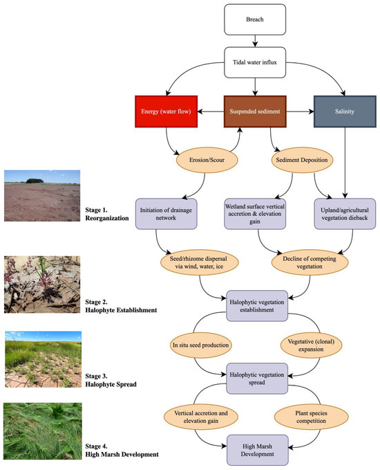
Figure 1.
Conceptual framework linking drivers of tidal wetland restoration following managed dyke realignment. Stages 1–4 follow [12].
Survival and expansion of tidal wetland plants on an MR site depends greatly on inundation frequency and duration [30,31] and thus ultimately on the elevation of the tidal flat or marsh surface [5,25]. Sediment accretion results from deposition of material from tidal waters and, in conjunction with organic matter accumulated by plant production, allows the wetland surface to rise in elevation [32,33]. Dykeland surfaces have often lost elevation over time due to lack of sediment inputs, compaction and altered drainage [34], whereas tidal wetlands are sinks for sediment suspended in incoming tidal waters and freshwater runoff from uplands [35]. In the upper Bay of Fundy, tidal wetland sediments originate largely from mineral material suspended in the water [36], thus deposition is important in determining the ability of a wetland to establish and to keep pace with sea level rise [19,32]. As tidal wetland plant communities expand, the role of plants in trapping sediments further increases elevation gain [32,37] (Figure 1).
The key processes of erosion and activation of the drainage network are governed by the energy of water flowing into the system. Flow velocity measurements at the creek mouth combined with an estimate of the cross-sectional area of the inlet allow calculation of discharge, the volume of water flowing in and out of the wetland (tidal prism) [15,25,38]. The amount of sediment in the water is quantified as suspended sediment concentration (SSC). Because of the importance of sediment deposition in the development of the new marsh, it is also desirable to calculate a sediment budget by quantifying sediment flux (the mass of sediment (SSC) travelling through the inlet [39] and subtracting flux out of the site on the ebb tide from the flux entering the site on the flood tide. Sediment flux may depend on season, as winter usually has a greater frequency of storms, which can result in higher suspended sediments and wetland surfaces, and lower vegetation cover and biofilm activity, leading to increased erodibility [38,40,41,42].
The effects of sediment dynamics are quantified by examining the change in marsh surface elevation. It can take up to 15 years for marsh surface elevation to stabilize following MR, and 60–100 years for equilibrium conditions to develop [43,44]. Repeated transect elevation surveys can provide an overview of net changes to elevation, but separation of aboveground processes, like sediment accretion, from belowground processes requires a more nuanced approach, such as using a combination of rod surface elevation tables (RSET), which precisely measure the elevation of the wetland surface relative to a fixed base [45,46], and marker horizons (MH), which measure the depth of sediments accreting on top of the original marsh surface after tidal restoration. Subtracting the magnitude of vertical sediment accretion from the elevation change quantifies the net effect of sub-surface processes, which include decomposition, compaction, groundwater flux and organic matter accumulation [45,46].
While MHs are usually sampled yearly, quantifying sediment accretion for individual tides can be accomplished by establishing sediment traps, where sediment accumulates on filter papers that are removed after each tide [47]. Similarly, RSET and MH techniques are precise but hard to replicate across a large area; digital surface models (DSMs) derived from repeated aerial surveys can provide estimates of vertical elevation change over the entire wetland surface when vegetation coverage is sparse or non-existent [48,49]. Drainage networks can also be mapped using DSMs, allowing assessment of the role of the evolving drainage network on the vertical growth of the wetland surface and vegetation establishment [23,50].
Quantifying landscape changes that accurately reflect such a dynamic system requires repeat surveys with varying resolution and precision, as well as varying technologies and survey methods. This is particularly relevant in the early years of restoration, where surficial sediments are very unconsolidated, with young seedlings establishing; both are highly influenced by physical disturbance, such as walking. Remote sensing techniques, such as the use of Remotely Piloted Aircraft Systems (RPAS), provide alternative methods for monitoring the morpho-dynamic processes of coastal wetlands, while reducing the need for researcher access to the marsh surface. Recent studies have only begun to utilize RPAS technology for measuring surface elevation change and drainage network initiation and development in salt marsh and mud flat environments [23,48,49,51,52,53], allowing repeated surveying at higher spatial resolutions than achievable with traditional survey methods. However, none of these studies incorporate detailed measurements of the sediment dynamics, which are driving the observed geomorphological changes [35].
This study applies recent advancements in RPAS technology to monitor and measure the ecomorphodynamic evolution and vegetation establishment of a restoring MR site in the Upper Bay of Fundy. The novelty of our work is the integration of measurements of sedimentary processes and hydrodynamics at a range of spatial (plot level to site wide) and temporal scales (individual tidal cycles, seasonal, annual) to inform the interpretation of changes we document using the RPAS technologies. We combined measurements of sediment flux and accretion, digital surface and drainage network models and vegetation mapping to understand the geomorphological evolution and vegetation dynamics at a MR site. The site had an area where the original agricultural surface was unaltered prior to restoration of tidal flow, as well as an area where the surface was altered by removal of vegetation and leveling (borrow pit). This allowed comparison between areas with legacy drainage and vegetation and those with a relatively clean slate. Given intermediate levels of suspended sediment in source tidal waters at the site, and recent agricultural history, we hypothesize that spatial variation in geomorphological evolution and vegetation establishment will depend on the presence of legacy features. In addition, the presence of only one tidal inlet (breach) and its erosion in response to high tidal current velocities provide an early sediment subsidy to the evolving marsh platform during over-marsh tides.
2. Materials and Methods
2.1. Site Description
The Converse dyke realignment and salt marsh restoration site is located within the Cumberland Basin in the Upper Bay of Fundy, Canada. The Cumberland Basin Estuary covers 118 km2 and approximately 2/3 of this area is occupied by salt marshes and mud flats [47]. Salt marshes in this region are exposed to semi-diurnal macro-tidal conditions, with a tidal range of 12–14 m [35], seasonally variable, high suspended sediment concentrations ranging from 0.05 g∙L−1 to 4.0 g×L−1 [36], and temperate weather conditions, with ice and snow present for at least 3 months of the year [47]. Salt marshes in the Cumberland basin are minerogenic, with surface elevation increases resulting primarily through sediment deposition rather than below ground biomass accumulation. Suspended and deposited sediments within the basin range in size from fine to coarse silt [36,54].
The study site runs along the eastern (Nova Scotia) side of the mouth of the Missaguash River, which represents the boundary with the province of New Brunswick (Figure 2). The original dyke protecting the agricultural land was experiencing extensive erosion, so the site was chosen for a MR and restoration project [55]. The site showed signs of subsidence behind the dyke prior to restoration, with a difference of ~45 cm lower on the agricultural surface compared to the fringe (foreshore) marsh [55]. Suspended sediment concentrations are intermediate (range: 0.08–2.0 g×L−1; [55].
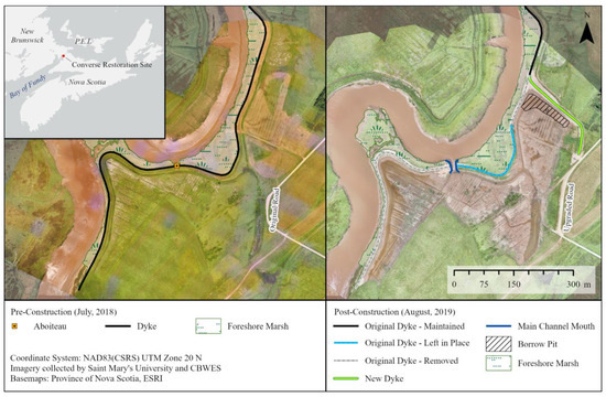
Figure 2.
Pre-construction (July 2018) and post-construction (August 2019) configurations at the Converse restoration site.
This project involved breaching a 420 m section of dyke in two locations, backfilling the removed materials into the drainage ditch inland of the original dyke to a surface elevation of ~5.9 m CGVD2013, and bringing the surface to the elevation of the natural foreshore marsh. This also included removing the existing aboiteau to allow the creation of a drainage outlet in its place (referred to as the main channel mouth) connecting the inner ditch to the main river channel. Prior to dyke breaching, 150 m of new dyke was constructed to a minimum elevation of ~7.2 m CGVD2013 to continue protection of adjacent dykeland. The new dyke was constructed using material taken from the agricultural field in front of the new dyke, referred to as a ‘borrow pit’, a portion of the decommissioned dyke and from an adjacent upland area (Figure 2). A section of the Fort Lawrence Road, which was below the Higher High Water Large Tide (HHWLT) elevation prior to restoration, was realigned and raised to a minimum elevation of ~7.2 m CGVD2013 [55]. These activities were completed by 21 December 2018, when the aboiteau was removed and first tide flowed into the site. Total restored area for this site was 15.3 ha, based on the area flooded at HHWLT (6.9 m CGVD2013) [55]. Relict agricultural ditches covered most of the site, excluding the borrow pit, where sediment was excavated and the remaining surface was flattened and graded (Figure 2), and a small pond for watering livestock occupied the southeastern corner of the site. There were also some remnants of natural salt marsh channels that pre-date the site’s agricultural history located south of the borrow pit (northeast section of the site). Hydrological flow onto the site is restricted by the main channel mouth on most high tides, but larger spring tides allow for over-marsh flow into the site in areas where the dyke was levelled/backfilled at peak water levels (Figure S1).
Elevation changes on the restoration site were quantified using transect surveys, digital elevation models (DEMs) from aerial surveys and RSETs [45,55]. RSETs and MHs were established in 2018 at four locations, one within the unmanipulated fringe marsh and three on the restoration site; three MHs were established adjacent to each RSET (Figure 3). RSETs and MHs were measured each fall beginning in 2019. Net accretion between years is determined by subtracting the current year’s measurement from the previous year’s. Three transects were established from the upland edge toward the fringe marsh and surveyed using the real-time kinematic global navigation satellite system (RTK GNSS) (Leica Viva GS14 GNSS Smart Antenna (Leica, Wetzlar, Germany), manufacturer’s reported positional accuracy of 11.35 mm horizontal and 18.35 mm vertical); three additional transects with permanent vegetation and sediment sampling plots were established (Figure 3) and all transects were sampled in 2017 (baseline/pre-restoration), 2019, 2020 and 2021. Twenty additional 1 m × 1 m vegetation plots were established in 2021 within the main restoration site for ground truthing of aerial imagery classifications. Detailed vegetation plot and sediment core data have been analysed in [55].
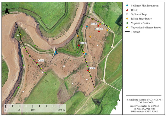
Figure 3.
Converse Marsh monitoring station layout including location of RSETs with MHs, vegetation plots, sediment flux instrumentation and rising stage bottles (RSB) locations.
2.2. Water and Sediment Flux
Sediment flux is defined as the amount of sediment travelling via tidal flow through a defined area [39]. In order to quantify sediment flux through the main inlet mouth, instruments were installed for five or six tides for each of three deployments that took place in August and November 2020 and July 2021 (years 2 and 3 post-restoration) [56]. High spring tides were targeted to make sure that the entire MR site platform was covered in water at high tide. Hydrologic variables, including water depth, velocity, and SSC, were measured over each tide at the main channel mouth to capture the temporal variations of inlet conditions. Cross-sectional measurements of the inlet were also taken for each deployment period. Additional velocity and SSC measurements were taken in the channels to help understand the dispersion of sediment throughout the site (Figure 3). At the main channel mouth, a Nortek Aquadopp Acoustic Doppler Current Profiler (ADCP)(Nortek, Boston, MA, USA), ISCO automated water sampler (Teledyne ISCO, Lincoln, NE, USA) and Ruskin RBR (RBR Ltd., Ottawa, Canada) were deployed. The ADCP was located on the floor of the inlet with the +X axis pointing downstream, aligned with the flow direction (Figure S2). The ground and ADCP sensor height were measured with an RTK GNSS for each deployment. The ADCP was programmed to take measurements every 10 s for 30 cells above the ADCP, set to 0.2 m in distance, totalling 6.2 m above the ADCP sensor. This height purposely exceeded the top of the main channel mouth and the highest potential tides. The ISCO automated water sampler pumped 500 mL water samples at 15-min intervals (Figure S3); a Ruskin RBR XR-420 was placed near the inlet, in the thalweg of the channel leading to the borrow pit, with the sensor 10 cm above the bed. Every 10 s during the deployments, it measured salinity (Practical Salinity Units: PSUs). Cross-sectional area of the main channel mouth for each deployment was determined from the DEM; discharge and sediment flux were calculated using the area of each ADCP cell and the SSC data from the ISCO for each completely submerged cell [56]. Average velocity of submerged cells for each timestep was used for depth averaged velocity (DAV).
To quantify sediment deposition on the marsh surface, sediment traps were deployed at eight locations throughout the site (Figure 3). Each trap consisted of a numbered Whatman 90 mm CAT5 filter paper (Cytiva Life Sciences, Vancouver, BC, Canada) set on top of a supporting 3M Scotch-Britetm heavy duty scouring pad (3M, St. Paul, MN, USA) between two aluminum sheets with a 90 mm circular cut out [38,40] (Figure S4). The traps were visually levelled upon deployment. After each tide, the filter papers were transferred to petri dishes and swapped for clean traps and filter papers. The filter papers from each sediment trap sample were dried and weighed to determine the deposition weight per unit area, using the pre-weights of each numbered filter paper and the effective area of the sediment trap (the cut-out area) where the sediment settled [38,40].
2.3. Aerial Surveys
Low-altitude RPAS surveys were conducted between July 2019 and July 2021 (years 1–3 post-restoration) with a DJI Phantom 4 RTK quadcopter (DJI, Shenzhen, China) at a flight altitude of 65 m above ground level. These flights were conducted with an oblique camera angle of 10° from nadir in order to allow vertical structures, such as channel banks, to be measured more accurately. An additional survey on 6 September 2022 (year 4 post-restoration) was conducted with a DJI Matrice 300 RTK quadcopter (DJI, Shenzhen, China) at a flight altitude of 80 m and a nadir camera angle. All surveys were conducted around low tide to maximize the amount of exposed sediment within the survey area, and covered a target area that included the borrow pit, main channel mouth, and the channel connecting both features. Ground control points were deployed on the site and measured with an RTK GNSS prior to each survey [57,58] (Figure S5).
2.4. Aerial Image Analysis
A DSM and ortho-mosaic were produced from the Structure from Motion (SfM) processing in Agisoft Metashape or Pix4D Mapper for each collection date (Figure S6). Products were exported with a pixel resolution of 2 cm (3.5 cm for the September 2022 survey). Vertical offset values between RTK GNSS validation points and DSMs for all collection dates ranged between −7.0 cm and 5.7 cm, and the average mean absolute error was 1.6 cm. The range in vertical root mean square error (RMSEz) was 1.3–3.3 cm. A Digital Elevation Model (DEM) was created for each survey by masking out water, vegetation and anthropogenic features in the DSMs, leaving only bare ground pixels.
Channels were delineated using a semi-automated method, scripted using Python (v. 2.7.16) and ESRI ArcPy tools (Figure S7) using November 2019, June, July, August, October, November 2020, May 2021 and November 2022 DEMs (only 2019 and 2022 results will be presented here). A flow accumulation threshold of 120,000 cells was used. Stream order was determined using the reverse order Strahler method [59], and the stream shapefiles were smoothed using the Paek method and a smoothing tolerance of 0.4 m. Stream segments were classified as either existent (>2 cm depth and connected to the rest of the existent channel network) or proto (<2 cm depth or disconnected from the existent channel network) (Figure S7) [60]. Since the script classified channels based on channel depth only, incorporating hydraulic connectivity and correcting erroneous classification results were completed manually post-classification.
Seasonal and yearly changes in surface elevation were assessed by calculating DEMs of Difference (DoDs) from the photogrammetric elevation models. For consistency in DoD extents, all DEMs were clipped to a minimum extent that represented only areas of overlap between all datasets. Resulting DEM rasters were subtracted from one another using the Raster Calculator tool to calculate surface elevation change over time per pixel for five intervals (Table 1) [52,53]. Volumetric change for each DoD was calculated by multiplying each DoD by pixel area and summing across all pixels in the dataset. Separate calculations were also performed for the borrow pit, main channel mouth and drainage channels (including the main channel mouth).

Table 1.
List of input DEMs for DoD creation, and representative DoD time periods.
To account for volumetric uncertainty in the above-mentioned datasets, a Level of Detection (LoD) was applied to all DoDs. This method of error estimation utilizes the individual DEM RMSE values and calculates their propagation into the DoDs using the following equation [61,62]:
where is the propagated DoD error and are the vertical RMSE values for the corresponding DEMs. LoDs were calculated for each DoD using the 68% confidence intervals, and volumetric change rasters were created incorporating each LoD threshold using the Raster Calculator tool by excluding all pixel values between (−)LoD and (+)LoD. The same procedure as outlined above for calculating total volumetric change was used for each of these volumetric rasters of “significant” change. Average vertical change for each dataset was compared across the datasets over the same interval using t-tests; within a dataset, average vertical changes were compared across intervals using paired t-tests. Multiple linear regression models were calculated in R [63] to predict surface elevation change (DoD rasters) based on starting elevation (DEM at beginning of interval) and distance from channel (DFC) rasters. DFC rasters were creating using the Euclidean distance to the closest channel classified as ‘existent’. The Create Random Points tool was used to select a series of randomly distributed points within the minimum DoD extent. The number of points selected was approximately 0.03% of raster cells within the specified extent. The residuals of each fitted model were inspected to assess homogeneity and normality. A log transformation was applied to predictors in cases where there was substantial deviation from the homogeneity of variance, and the models were re-run with the transformed datasets. Both predictor variables were scaled (converted to unit variance) so that coefficient magnitudes could be directly compared. Predictors in all models were screened for co-linearity by calculating variance inflation factors, and models were run if all variables showed variance inflation factors < 10. Cross validation was completed to estimate the prediction error of each model and the magnitude of effects of spatial auto correlation was assessed using variance partitioning [64]. Three intervals for DoD calculation were examined in this analysis: 1-year (24 November 2019–5 October 2020), winter (24 November 2019–1 June 2020), and growing season (1 June 2020–5 October 2020).
2.5. Vegetation Mapping and Classification
Twenty additional 1 m × 1 m vegetation plots were established on the restoration site in summer 2022, stratified by 0.5 m elevation intervals from the 2021 DEM and georeferenced with the RTK GNSS. Each vegetation plot was divided into a grid of 25 20 cm × 20 cm squares and the presence of each species within each square recorded. Aerial images from 24 September 2018, 16 July 2019, 21 August 2020, 25 July 2021, and 6 September 2022 were used to track vegetation changes. Supervised object-based classification used the dominant species (most abundant) from the 20 vegetation plots (40 plots in 2022) as a training set for each year. The classes “brackish grasses”, “early establishers”, “Sporobolus alterniflorus”, “high marsh” and “Sporobolus michauxianus” were grouped as a combined “halophytic vegetation” class to evaluate the spatial persistence of halophytic vegetation. Since calculating a DoD requires masking the vegetated areas within the DSMs to create DEMs, the new shapefiles had to be paired with the previous year’s DoD to obtain valid bare ground data beneath the vegetation features, so persistence and elevation change rates could only be calculated for 2021 and 2022. Areas of halophytic vegetation persistence were determined by comparing the halophytic vegetation extent for each year and identifying areas of overlap. New growth was determined from 2020–2022 using the extracted halophyte feature classes in the first step and the persistent halophyte feature classes. All halophytes from 2020 represented new colonization; therefore, the extracted halophyte class in the first step represented new growth. New colonization/expansion was determined in 2021 by subtracting the persistent vegetation from the total halophytes in the study area, leaving only new colonization in the output layer.
3. Results
3.1. General Restoration Trajectory
In the first year post-restoration (2019), there was limited colonization by tidal wetland vegetation; however, there was sediment deposition on the former agricultural surface and dieback of agricultural species, resulting in a surface mostly covered with sediment (Figure 4). The breach channel increased in cross-sectional area, widening slightly, but had mostly eroded down to the remnants of the aboiteau. The re-introduction of tidal flow initiated a relict and hybrid drainage network in the first year. Revegetation was slow over the first three years but by 2022 the site was mainly covered with various types of tidal wetland vegetation (Figure 4). Elevations increased throughout most of the site (Table 2). Elevation loss was mainly restricted to the primary tidal channel, with elevations on the western bank of the channel mouth lower by up to a meter. Elevation loss was also observed on the platform near the channel mouth. Notably, the borrow pit experienced the most deposition, increasing in elevation by 40 cm or more in some locations. Areas with remnant agricultural ditches typically maintained their position over time as part of the channel network, following the right angles and straight lines of the relict ditch network (Figure 5). New channels with more sinuous patterns developed within legacy natural features and embryonic channels also developed in the borrow pit area (Figure 5). Areas such as the borrow pit were faster to establish channel networks, despite higher-than-average rates of sediment deposition in this area.
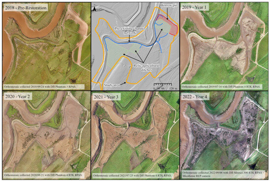
Figure 4.
Development of the Converse Marsh from 2018 pre-restoration to 2022-Year 4 post restoration.
Table 2.
Elevation statistics from transects surveyed with an RTK GNSS [55]. Elevations relative to CGVD2013, 2017 data are considered as “pre-restoration”.
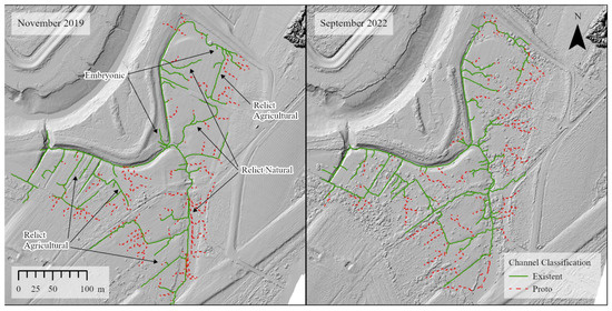
Figure 5.
Drainage networks in November 2019 and September 2022. 2019 map annotated to show examples of relict agricultural, relict natural and embryonic channels.
Surface and subsurface processes both affected elevation changes within the restoration site. In the first year, the largest increase in surface elevation occurred at RSET-1 at the western end of the restoration site; the lowest within the restored area was at RSET-3 closest to the borrow pit (Figure 6). Approximately half of the Year-1 surface elevation increase at RSET-1 can be attributed to sediment accretion (3.71 ± 0.2 cm∙a−1), with the remainder (3.3 cm∙a−1) associated with below ground processes (Figure 6). The substrate consisted primarily of old pasture grasses overlain by bare mud. RSET-2 showed a negative net elevation change between years 2 and 3, but a positive accretion value over the interval. This means that elevation losses due to processes operating below the MH were greater than the elevation gain from sediment accretion. Negative belowground change at these two stations in 2020 and 2021 may have resulted from collapse of air pockets created by initial burial of pasture grasses by sediment and thus, despite net positive accretion, the surface elevation increased only slightly, or sank relative to the previous year’s measurement. Accretion values for the three stations on the restoration site were generally higher than at the reference station RSET-4, although RSET-3 showed some loss of previously deposited sediments between 2020 and 2021. RSET-4 on the natural foreshore marsh recorded yearly elevation increases between 0.7 and 2.2 cm (Figure 6). Overall, the net positive elevation changes were mainly due to sediment accretion, which usually exceeded the belowground changes that reduced elevation (Figure 6).
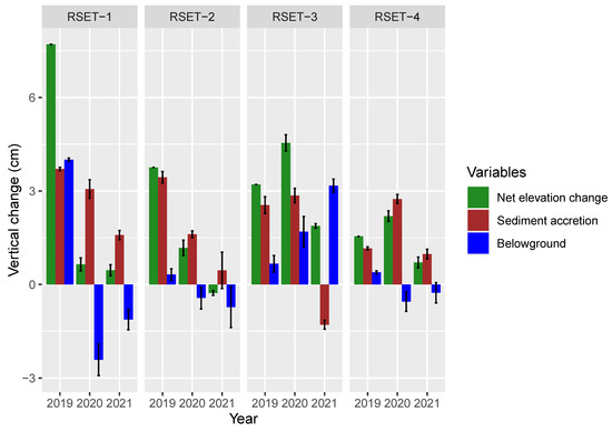
Figure 6.
Vertical change of the marsh surface at Converse restoration site measured at RSET stations. Yearly values represent change in elevation or accretion relative to the previous year’s measurement. Net elevation change measured from RSETs. “Accretion” represents the net amount of sediment deposited on the surface (accumulation of sediment above the MH); “Belowground” represents net change due to changes below the MH (Net elevation—Accretion).
3.2. Hydrology, Inlet Evolution
While the instrument deployments in August and November 2020 and July 2021 all occurred during Spring tides, they differed in position within the perigean-spring tidal cycle (Figure S8). The November deployment was almost at the height of the 206 day, perigean-spring cycle and had the highest tides recorded. August was closer to the middle of this cycle and July 2021 closer to the low point. Based on the predicted maximum tide heights (obtained through the Canadian Hydrographic Service (CHS station 00190, [65])), approximately 15% of tides during the deployments flooded the entire marsh surface (bank-full conditions at 5.9 m CGVD2013) (Figure 7). The salinity of the water entering the site from August 2019 to July 2021 ranged from 19 to 31 PSU (Table S1).
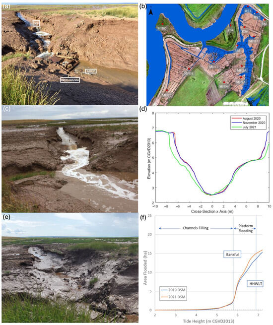
Figure 7.
Inlet evolution: (a) inlet in August 2020 (20 months post restoration) showing instrument locations; (b) site flooded to bank-full level (5.9 m CGVD2013); (c) inlet in November 2020; (d) cross-sectional data of inlet for each deployment; (e) inlet in July 2021; (f) hypsometric curve showing area flooded at tide height with critical elevation thresholds indicated.
Within the first two years of re-introduction of tidal flow, approximately 126.6 ± 8.0 m3 (95% CI) of sediment was eroded within the mouth of the channel inlet [60]. There were changes in the cross-sectional area of the inlet between each deployment as it eroded and evolved. The inlet was smallest in August 2020, then slightly widened by the November 2020 deployment (Figure 7), with an approximate cross-sectional area of 50 m2. There was more noticeable widening to approximately 55 m2 in the 8.5 months leading up to the July 2021 deployment (Figure 7); the inlet/V3 area also became more smoothly sloped toward the inlet (Figure 7). Within deployments, maximum flood and ebb velocities increased with increasing tidal water surface elevation. In August, the inlet current velocities on the ebb tide were noticeably higher than in November 2020 and July 2021, seen in the average depth averaged velocity. The maximum depth averaged velocity of the August ebb tides were over 1 m∙s−1 and matched that of November, which came from the observed 7.04 m tide (Table 3). August had the highest individual cell velocities of 2 m·s−1 at the surface, almost reaching the thalweg. November Tide 4 matched these velocities, reaching 2 m·s−1 at the thalweg (Figure 8), possibly creating scour; November flood tide maximum discharge values were almost double the maxima for the summer deployments (Table 3). The flood and ebb velocities grew weaker after the August deployment, with the exception of the 7.04 m November tide.
Table 3.
Hydrology and sediment variables recorded at the inlet mouth at Converse restoration site.
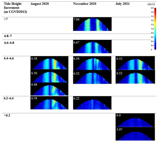
Figure 8.
Velocity plots (from the Storm64 program) showing velocity of the rising and falling water, with height relative to the ADCP. Plots are divided into maximum tide height increments.
Generally, similar tides had similar discharge values, regardless of velocities, indicating interactions with the cross-sectional area. November 2020 had the highest average and maximum discharge for the flood and ebb tide (Table 3). August 2020 and July 2021 had similar maximum flood and ebb discharge values, but August had higher average values. All deployments had higher SSC values on the flood tide, except for the end of the November tides (Table 3). SSC differences are seen between November and August, where the maximum flood SSC was around twice as high in November (Table 3). However, July had nearly the same maximum flood values as November, likely due to a heavy rain event prior to one of the July tides (Figure S9). Instantaneous sediment flux exhibited similar patterns to those of velocity and discharge (Table 3).
Deposition onto sediment traps varied between tides and deployments (Table 4); the proportion of traps receiving deposition ranged from 57% on the lowest tide to 100% of stations for 6 of the 13 tides. November received the most deposition on average and August received the least (Table 4).
Table 4.
Maximum, minimum, and average deposition values for each deployment (g·m−2) per tide.
3.3. Surface Elevation Change
The 1–2 years post-restoration DoD (Figure 9) shows mostly positive surface elevation change in the borrow pit and field area just south of the borrow pit. The majority of positive values in these areas ranged between the LoD (2.5 cm) and 10 cm, but there were some small areas of between 10 cm and 50 cm of surface elevation increase in the borrow pit. The southwest part of the site representing the old agricultural surface showed mainly small negative change (decrease in elevation) but most of these areas saw change not exceeding the LoD. Over the entire MR site, vertical change and volumetric changes were net positive for the entire year, net negative for winter, but net positive for the growing season (Figure 10). For both variables in the whole site analysis, whole year and winter confidence intervals overlap zero (Figure 10). Borrow pit vertical and volumetric changes were net positive, and higher in winter than growing season (Figure 10). Both drainage channels and the main channel mouth had net negative change for the whole year and winter datasets, contrasting with net change of around 0 for the growing season (Figure 10).
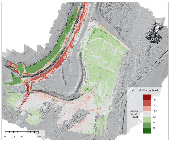
Figure 9.
DoD raster showing surface elevation change from 24 November 2019 to 5 October 2020 (1-year). LoD was calculated using a 68% confidence interval. Background is a hill-shade of the 5 October 2020 DSM.
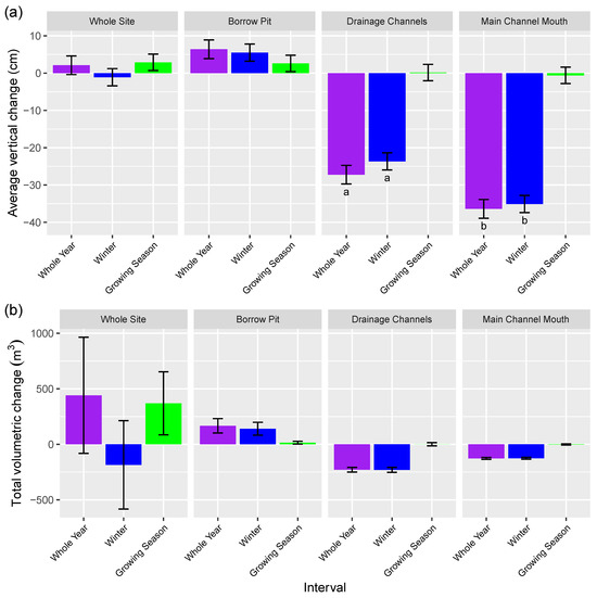
Figure 10.
Vertical and volumetric change calculated from DoD, using a level of detection based on a 68% confidence interval. In (a), all averages are significantly different from one another (p < 0.0001), except those sharing letters; Error bars: Volumetric uncertainties (b) were calculated using the equation in [66], and vertical change uncertainties (a) were calculated by dividing the volumetric uncertainty by area. Whole year: 24 November 2019 to 5 October 2020; Winter: 24 November 2019 to 1 June 2020; growing season: 1 June 2020 to 5 October 2020.
Predictive modelling of elevation change showed a similar pattern for most datasets: a strong negative effect of elevation (higher elevations gained less elevation), a positive, but weaker effect of DFC (areas farther from the channel gained more elevation) and a significant interaction effect (Tables S2–S13). Interpreting the interaction effect, the whole year and winter models showed similar results, with the overall effect of elevation on surface elevation change being negative at all DFC values, but the overall effect of DFC was positive below a certain elevation threshold, and negative above this threshold. The overall effect of DFC on surface elevation change was positive in both growing season models. The overall effect of elevation on surface elevation change was consistently negative in the borrow pit growing season model. Spatial autocorrelation was detected in each of the multiple regression models, with variance partitioning indicating that the majority of the variance explained by the fixed effects in the model should be considered as spatially structured environmental variation [64] (Tables S3–S13). Further modelling has suggested that, when spatial autocorrelation terms are added to the multiple regression models, p-values and coefficients are similar to those presented here (Tables S2–S13).
3.4. Vegetation
In 2019 (Year 1 post-restoration), the site was dominated by bare ground (~85%), with remnants of the pasture vegetation persisting (~15%) (Figure 11). In 2020, bare ground remained dominant in the site (~81%), though the agricultural/pasture vegetation had largely been replaced by Sporobolus michauxianus and dead material (Figure 11). The first notable establishment of halophytes was evident in 2020 (Figure 11 and Figure 12), though 10% of the study site was still characterized by dead vegetation (Figure 11). New halophyte establishment totalled approximately 10% coverage in 2020. By Year 3 post-restoration (2021), the site had reduced to approximately 40% bare ground, with approximately 47% of the area covered by new halophytes, and 9% coverage of halophytes established in the previous year (Figure 11). There appeared to be rapid establishment of halophyte species, notably Sporobolus alterniflorus (5%) colonization in the center and northwestern section of the site, and bare ground dominance shifted toward early establisher (halophytic annuals) dominance (30%) (Figure 11 and Figure 12a). By 2022 there was a reduction in coverage by early establishers and increase in target species S. alterniflorus to approximately 15% cover, with 36% cover from previously established and 23% from newly established halophytes (Figure 11 and Figure 12). Vegetation plot data confirms large increases in species richness, total plant cover, halophyte richness and abundance between 2020 and 2021 [55]. Multivariate analysis confirms that the vegetation had shifted from agricultural/pasture species to dominance by native tidal wetland species by 2021 [55].
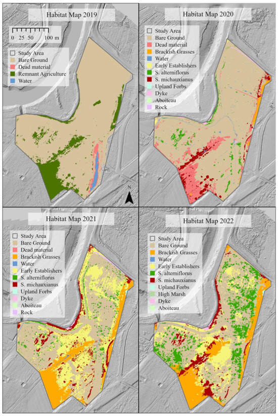
Figure 11.
Habitat map of the study area within the Converse Marsh from 2019 to 2022 (Year 1 post-restoration to Year 4 post-restoration). “Brackish Grasses”: Agrostis stolonifera, Elymus repens. “Early Establishers”: Suaeda spp., Salicornia spp., Atriplex spp. “High Marsh”: Sporobolus pumilus, Juncus gerardii. “Upland forbs”: Trifolium spp., Solidago spp. etc.
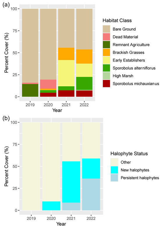
Figure 12.
Stacked bar charts representing the (a) percentage cover of each class within the study area from year 1 post-restoration to year 4 post-restoration; (b) the abundance of ’other’ cover (includes bare ground, dead material and agricultural vegetation), persistent halophytes, and new halophytes (new growth) from Year 1 post-restoration (2019) to Year 4 post-restoration (2022).
Establishment of halophytic vegetation in 2020 occurred in higher elevation areas, particularly toward the outer bounds of the study site (Figure 13). S. michauxianus appeared to grow dominantly in a linear pattern, particularly adjacent to ditches along the west side of the site (Figure 13). New growth and establishment the following year demonstrated greater variability in patches. Expansive patches were notable in the center of the site, which were dominated by early establishers (Figure 11 and Figure 13). There was also evidence of clonal spread, particularly by S. alterniflorus, as patches in 2020 developed rings of new colonization around them in 2021 (Figure S10). In the eastern section of the site, there appeared to be linear spread of halophytic vegetation along relict agricultural ditches (Figure 13). Year 4 post-restoration (2022) exhibited less new establishment. However, it was notable that small patches of S. alterniflora tended to merge and form larger patches of dense monocultures in the center and western areas of the study site (Figure 11). Vegetation establishment appears to be associated with channel networks in 2020 (Figure 13) but newly establishing vegetation in 2021 and 2022 does not show such an association (Figure 13). Cracks in the surface of mud flats in the borrow pit and other areas also saw establishment of S. alterniflorus by 2022 (Figure S11).
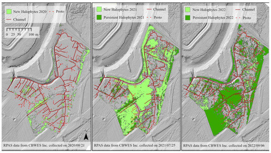
Figure 13.
Relationship between channel networks and vegetation colonization in from 2020 to 2022. Light green represents new colonization, dark green represents persistent vegetation, solid red lines represent channels and dashed red lines represent proto-channels.
4. Discussion
The ecomorphodynamics and evolution of tidal wetland landscapes reflect a complex interaction of sedimentary, hydrodynamic and vegetation processes that change over time [35]. Restoration of tidal hydrology created three important inputs to the Converse MR site. The energy from renewed tidal flow drove the geomorphic evolution of the site, reconfiguring the inlet, provided an initial sediment subsidy as it eroded, and drove rapid development of a drainage network. This led to rapid deposition of sediment to much of the site. The RSET results and DoDs suggest that, overall, the site has experienced vertical growth over the first four years post-restoration at a rate that exceeds sea level rise (approximately 0.004 m∙a−1) [67]. At sites where early deposition of sediment is very high, this can create a clean slate for rapid establishment of tidal wetland vegetation [26]; however, at Converse, the depth of accreting sediment was not high enough to create such a clean slate effect, except in the borrow pit area, where prior vegetation was removed. The first areas where halophytic vegetation established were areas that showed remnant agricultural vegetation in 2019 and mainly dead vegetation in 2020 (and were not covered by sediment; otherwise they would have been classified as “bare ground”) (Figure 11). This points to the influence of the third input, i.e., salinity from tidal waters, which was likely responsible for killing off legacy vegetation that was not buried under sediment [27]. The initial elevation of the marsh platform is also an important conditioning variable on vegetation recovery; it was the highest elevations that were not completely covered with sediment where new vegetation first established, resulting in brackish vegetation by 2020–2022 (Figure 11). The vegetation maps also reinforce the role of the drainage network in fostering tidal wetland vegetation establishment where new tidal wetland vegetation first established along the creek network. The Converse Site is following similar restoration trajectories reported in other management realignment sites in the Bay of Fundy [12,26,68] and in Europe [23,24,25,69], and our work provides one of the most comprehensive field studies of the co-evolution of the salt marsh landscape and halophyte establishment and spread.
4.1. Geomorphological Evolution and Re-Organization
The initial re-introduction of tidal flow in December 2018 stimulated initial erosion at the channel inlet and significant downcutting of a drainage ditch that preceded this study [70]. This initial erosion and self-engineering provided an initial sediment subsidy to the former agricultural surface. Inlet erosion and internal adjustment associated with increased tidal flow is well documented in previous studies [23,51,71]; however, this contribution and provision of a sediment subsidy is rarely documented. Significant external erosion noted in [15] was not observed at the Converse site. Therefore, our study suggests that deliberate under-sizing of inlet dimensions to allow for erosion and self-organization could be an important design element in future MR schemes.
Combining detailed measurements of water velocities and sediment flux at the site inlet with extensive aerial capture of DEMs over time can help explain the importance of seasonal variation to the evolution of the site. A recent numerical model with an unstructured flexible mesh (Delft3D-FM) was applied to the Converse site to simulate the hydrodynamics inside and around the breach before and after tidal flooding during spring tides, to evaluate the initial impacts of MR [72]. Maximum modelled discharge into the site (23 m3∙s−1) aligned with measured values on flood tides; however, modelled ebb velocities as water drained the site were underestimated compared to recorded values in our study. This is likely due to the model grid resolution, which may not be able to adequately reflect drainage through narrow, deep agricultural ditches. Model results demonstrate that the initial fast incoming currents can exceed 1.0 m∙s−1 through the breach and then decrease as water is spread over a large area, with an average depth of 0.66 m over the newly restoring marsh platform, and current speeds decrease to below 0.3 m∙s−1 [72]. This is sufficient to allow for sediment deposition on the marsh surface as observed within our study and is within the range of velocities over the marsh surface recorded in other studies in the Bay of Fundy [38,47].
Hydrodynamic conditions at the inlet varied temporally over each tide and between deployments during one year of site evolution. The larger perigean-spring tides had higher velocity and SSC values, thus experiencing a higher influx of sediment through the inlet, but average velocity decreased over time in tandem with the widening inlet [73,74]. Higher velocities result in higher SSC from resuspension [75] during tides with peak velocities around 1 to 1.2 m∙s−1 [76]. Higher amplitude tides cause higher SSC values on natural marshes [77,78], because of these higher velocities and the erosion of mudflats fronting them [76,77,78,79]. SSC also increases from the erosion of tidal channels experiencing high velocities. Studies have previously attributed higher SSC and deposition to certain seasons because of weather and biological factors [80,81,82,83,84]. Reductions in SSC and sediment flux as the site developed and velocities decreased could not be confirmed using results from sediment traps due to precipitation before the last deployment, raising ambient SSC; however, RSET and MH results showed decreasing accretion rates accompanying lower rates of elevation change over the first three years post-restoration (Figure 6).
The large perigean-spring tide recorded resulted in the largest import of sediment and redistribution within the site. While the deployments generally coincided with relatively high tide and energy conditions, velocities above 1 m∙s−1 were only detected in tides above 6.2 m CGVD2013, which are infrequent at the site; thus, relatively few tides are likely to be responsible for the geomorphological changes seen at the site (Figure S9), matching previous studies [14,78]. Over time, the inlet’s morphology will adjust to an equilibrium form and provide less sediment input onto the marsh platform. This inlet will respond to future changes in hydrology (increased tidal prism with sea level rise, intensive pluvial events) or climate (changes in ice conditions) by adjusting its form, potentially triggering another cycle of erosion and sediment input.
The DoD analysis, however, confirms that winter was associated with more negative changes to elevation (outside of the borrow pit area), on large areas of the flat which were previously agricultural surface, likely to be due to the settlement of air pockets (false surfaces) described above. However, in in-channels and at the main site inlet, negative elevation likely results from increased erosion due to greater maximum discharge rates in winter, as well as the effects of ice blocks (Figure 10). Increased SSC in the Bay of Fundy in the winter [38,42] is expected to increase sediment deposition rates [85] and surface elevation change. In the borrow pit, all DoD time periods resulted in a net gain of surface elevation, with the highest gain occurring over the winter as expected, and measured deposition in sediment traps was also higher during the November deployment than either of the two growing season deployments. Given confirmed sediment deposition at the site in winter and the small magnitude of negative change detected (confidence intervals overlap zero) for the whole site dataset in contrast with the borrow pit, where legacy vegetation was removed, this suggests that the negative vertical change was an artifact driven by the areas of the site that had legacy agricultural vegetation. The main channel mouth was characterized by net erosion (surface elevation decrease) throughout the year, with the highest magnitude of change occurring over the winter. The volume of sediment influx to the borrow pit was slightly higher than sediment loss in the channel mouth over all time periods, indicating that some sediment is entering the site from other areas; however, the magnitudes are very similar (Figure 10b), indicating a potentially major role of erosion at the single tidal inlet as a sediment subsidy to the marsh platform in early restoration. Previous work has identified sediment accretion rates in other borrow pits in the Bay of Fundy as varying significantly, ranging from −0.54 m×y−1 to 0.18 m×y−1 [52], with results from this study falling within that range. The amount of vertical change in the borrow pit was similar to sediment deposition values collected at the Aulac MR site just north of Converse in the second year of restoration [12], as well as sediment accretion values for the same time period measured at the Converse restoration site using MH [55]. Daily sedimentation rates at the Converse site were markedly higher (360 to 620 g∙m−2 per day) than those recorded using sediment traps in the Perkpolder site (100 g∙m−2 per day) in the Netherlands by [25], despite not being situated at the maximum estuarine turbidity.
Sedimentation is critical to allow for the subsided formerly dyked agricultural surface to rise within the tidal frame to an elevation that can support the establishment of halophytic vegetation [12,24,26]. The regression models linking elevation and distance to channels with elevation change confirm the negative relationship between elevation and sediment deposition (Tables S2–S7), likely due to the negative relationship between inundation duration and elevation [86], thus opportunity for deposition is decreased at higher elevations. A similar general principle is probably at work explaining the positive relationship between distance to channel and vertical elevation change: at a given elevation, areas closer to the channel obtain less sediment as velocities are higher. However, because the drainage network was studied at early stages of its evolution, the interaction effect detected suggests that, very close to the channel, the highest velocities result in lower net gain in elevation due to a combination of active erosion of channel sides and higher velocities, reducing opportunities for sediment to settle. This results in an optimal distance from the channel for maximal deposition with declines farther and closer to the channel. This may contrast with mature sites, where channel erosion has largely ceased [38]. Sediment trap results show overall higher deposition during tides with greater sediment flux, indicating the dependency of accretion on SSC in the channels, which are important conduits for the delivery of sediment to the marsh surface. The approach here used a simplified statistical modeling framework that incorporated only two variables; further modelling efforts are indicated and could benefit from incorporation of theory and a more complex set of predictor variables [72,87].
4.2. Effects of Legacy Vegetation
Differences in vertical growth at the marsh surface and vegetation recovery were attributable to spatial variability within the site, caused by the elevation gradient but also by the geomorphological interventions in the borrow pit area on the north side of the site. The areas on the southeastern section of the site had remnant vegetation from the agricultural surfaces at the time of hydrological restoration, leading to a layer of sediment on top of dying pasture grasses. The sediment was not heavy enough to fully compact the vegetation layer, in contrast to sites with larger initial sediment accretion [26], resulting in pockets of air between the actual ground surface and sediments that had been deposited. This would have created false surfaces in some areas of the DSM that were not accounted for in processing. During winter 2019, additional deposited sediment as well as snow and ice may have increased compaction forces on the vegetated layer, reducing air pockets and lowering sediment surface elevation, as measured in June 2020. In the resulting winter DoD, these areas were characterized by surface elevation loss, but that loss may have been a result of compaction rather than sediment erosion; those areas may have actually had considerable amounts of sediment deposition. In the borrow pit, where agricultural vegetation had been removed during excavation, deposited sediments caused surface elevation to increase, resulting in the net volumetric gain as calculated for all time periods.
Erasing the legacy of pasture vegetation and lowering of the surface elevation by excavation of the borrow pit and subsequent leveling of the north portion of the site avoided the problem of poor conditions for plant growth caused by air pockets or decomposing vegetation, but that section of the site also had relatively slow plant recovery. In this case, it took several years for elevation to build up to support vegetation establishment and this was also seen at the nearby Aulac restoration site [12]. Microtopography in newly restored salt marshes has been shown to facilitate the re-establishment of pioneer species through seed entrapment, as well as the provision of favorable water relations for seedling establishment [88]. S. alterniflorus and early establishers were consistently close to channels (<10 m), which is likely to be highly influenced by their tolerance for high saline environments and frequent tidal inundation compared to other species, but is also possibly a vector for seeds and rhizomes to reach the site. This is especially important, as initial colonizers tend to facilitate the establishment of other perennial halophytes as they facilitate sediment trapping, raising the elevation in the tidal frame and creating more favourable conditions for later successional species, the high marsh dominant S. pumilus [12]. The patterns evident in the habitat maps show that the remnant agricultural channels are more associated with new halophyte establishment than new channels. The borrow pit area was the last to be colonized by plants, possibly due to the time required for the surface elevation to build up, the erasure of previous legacies or the initial lack of surface microtopography, although surficial cracks in the sediment surface also showed halophytic plant establishment occurring by 2022.
4.3. Effects of Relict Hydrological Features
Comparison of channel delineations from multiple collection dates indicated an early initialization of drainage networks and the general stability of these networks throughout the study period [55,60]. The developing channel network has incorporated relict agricultural features where present, but also some relict natural features, and embryonic channels have developed where the effects of the antecedent landscape history were not present. Channels developing within the borrow pit were characterized by a sinuous appearance and differed from the majority of channels within the rest of the site that incorporated agricultural ditch features. This is similar to findings by [23] in the UK and [25] in the Netherlands. Lowering of the surface elevation by excavation of the borrow pit and its connection to the river allowed for frequent flooding, resulting in a morphological evolution that more closely resembled natural salt marsh processes. More research is required to determine differences in long-term trajectory within the borrow pit and the remainder of the Converse restoration site.
Overall, the site’s drainage network was relatively stable throughout the study period and the ultimate channel network patterns imprinted within the first year of tidal flow. Since the channel study began almost one year after the initial introduction of tidal waters to the study site, measurements of channel initialization in the first year of restoration could not be conducted, but a related modelling study showed that velocities in the first year were sufficient to cause erosion, with a maximum discharge of 23 m3∙s−1 [89]. RPAS data collected during the 2019 field season as part of the site monitoring project and other research activities provided additional insights into channel evolution. There is general alignment between channels present just a few months after the site breach and the delineation, demonstrating that embryonic channels in areas unaffected by relict landscape features established rapidly [70]. This finding agrees with modelling results [90], as well as empirical study results [23], in which channel networks had begun establishing within an MR site in the UK within 1 year of site restoration. Once established, the persistence (and deepening) of tidal channels in the evolving marsh surface align with tidal creek evolution reported in young natural marshes [91]. However, some shallow ditches in the western section infilled, re-directing draining tidal waters to adjacent deeper ditches.
4.4. Halophyte Establishment and Spread
The development of vegetation at the Converse restoration site aligns well other studies in the Bay of Fundy [12,26,68]. In the Aulac MR site, four stages of vegetative community succession were recognized: (i) initial rapid deposition of unconsolidated sediment and loss of terrestrial vegetation with remnants of S. michauxianus persisting (1 y post-breach), (ii) establishment and spread of S. alterniflorus and loss of S. michauxianus (2–5 y post), (iii) high percentage cover and decreased spatial variability of S. alterniflorus, and (iv) maturation of sediments and encroachment of high marsh [12]. First and second years post-restoration at Converse show a similar trajectory, characterized by limited establishment of target halophytic species, with remnants of the site’s agricultural vegetation persisting and a marsh surface of mainly bare ground from deposited sediment. The initial low abundance of halophytic vegetation early in the restoration trajectory is well supported in the literature [12,26], and at Converse may be due to the decomposing layer of dead vegetation and wet conditions that gave rise to an anoxic environment [92], or a negative effect of air pockets on plant growth. The effects of the legacy of dead pasture vegetation also suggest that mowing the site prior to restoring tidal hydrology may result in faster colonization by halophytic vegetation.
Year 2 post-restoration demonstrated initial colonization of halophytic species, primarily, S. alterniflorus, S. michauxianus, and early establishers (annuals). Given the proximity of the intact fringe marsh, it is likely that these species reached the site by seed transport. This was supported by the small circular patches that were present on the mudflat in the center of the site. However, there were also larger patches of S. alterniflorus that had not been present the previous year, suggesting that rhizome material of S. alterniflorus was deposited via winter ice blocks [28,71,93] or tides [12], which is a common phenomenon in the Bay of Fundy.
As the site accreted sediment and became more stable, it created more favourable conditions for plant establishment, which was more evident in Year 3 post-restoration: early establishers such as Suaeda spp. dominated the site and bare ground area was reduced by nearly half. Salt marsh annuals (Suaeda spp. and Salicornia spp.) have been recorded as the earliest colonists in other studies [94,95,96,97]. The expansive patches of annual halophytes represent primary salt marsh succession. Their presence promotes sediment accretion and facilitates the establishment of target perennial halophytes that characterize later successional stages [92]. This was demonstrated in Year 4 post-restoration as S. alterniflorus represented a larger portion of the site and had begun to replace Suaeda and other annuals in lower elevations. Development of high marsh, characterized by Sporobolus pumilus and Juncus gerardii that became common by Year 4, is characteristic of the fourth phase of succession [26]. This suggests that the Converse restoration site achieved each successional stage within a 4-year time frame and is on a positive trajectory towards complete restoration.
S. alterniflorus showed a shift from establishment of individuals via seed or rhizome, to clonal spread from established patches in later years, a phenomenon also reported in other studies [95]. There were several indicators of clonal spread of vegetation, particularly by S. alterniflorus. First, there were patches that grew larger surrounding rings of vegetation in consecutive years [93]. Next, the prominent straight lines emerging from the mature patches of S. alterniflorus (Figure 11 and Figure S10) would eventually merge with nearby patches to form monospecific populations [68].
4.5. Utility of RPAS for Monitoring Restoration Trajectories
An RTK-enabled RPAS was utilized in this research, along with SfM workflows to conduct multi-temporal aerial surveys of a restoring MR site on the Bay of Fundy, Canada, to measure changes in surface elevation and to map drainage networks. Accuracies of the collected datasets were high compared to results from similar studies in salt marsh systems [23,51,52,53,98], allowing for the measurement of fine-scale changes and details within the site. Nevertheless, there were clear limits to the use of these techniques, especially for assessment of volumetric change. As calculated volumetric uncertainty at those scales often exceeded measured volumetric change, it is recommended that future volumetric change calculations in MR sites with similar sedimentation rates be limited to small areas of interest in which expected surface elevation change is significant (e.g., majority of cells greater than LoD), such as a borrow pit (area of relatively lower elevation) or channel mouth (area of high erosion), or be conducted over time periods ≥ 1 year. An additional concern in conducting DoD analyses to calculate volumetric change is the nature of surface elevation change measurements. Surface elevation change in a salt marsh system is comprised of both above ground and below ground processes. Above ground processes include sediment accretion and erosion, and below ground processes include below ground biomass growth, compaction, and water saturation [32,99]. Converting surface elevation change to sediment volumetric change (an above ground process) automatically assumes that below ground processes are negligible. This was not the case, however, at the Converse restoration site, where compaction of agricultural vegetation was identified, and other types of below ground processes may have been occurring. Finally, the DSM error estimation method used in this research was the calculation of a single error value for each surface model. While this approach is generally accepted and utilized in the literature, several studies have recommended the use of spatially variable error estimations [100,101,102] to better represent the non-random, spatially correlated error present in SfM elevation models. The application of a spatially variable error estimation method for RPAS datasets in this research may have reduced the issues encountered with directionality of error in some parts of the study site and false surface elevation change measurement. It is recommended that spatially variable error estimation techniques be researched to determine their applicability for RPAS surface models and, if appropriate, incorporated into further DoD and volumetric change analyses. Further modelling of sediment dynamics should combine sediment elevation change assessed from RPAS data with intensively sampled sediment traps and other point measurements.
4.6. Effects of Tidal Wetland Restoration on Ecosystem Services
Tidal wetland restoration via MR is expected to increase the provisioning of particular ecosystem services [9]. At the Converse MR site, the vertical gains of the marsh platform accompanied by increased vegetation cover suggest that the site has gained resilience in the face of SLR due to less potential for erosion. Plant cover also contributes to wave attenuation [6,9], which enhances coastal protection. The surrounding area is mainly agricultural, so the increased coastal resilience provided by the new salt marsh as well as the new dyke are expected to contribute to sustained or increased agricultural production in the local area. While fish populations were not monitored in this study, other MR projects in the upper Bay of Fundy show that salt marsh restoration results in relatively rapid onset of use by fish of commercial and cultural importance [27,71], typically as nursery habitat. The relict agricultural ditches are likely to have fostered vegetation recovery via provision of spatial heterogeneity [94] and dissemination of seeds or vegetative propagules, enhancing the site’s ability to provide coastal protection and habitat for food fish. Ecosystem services tied to wetland vegetation might be improved early in the restoration trajectory by mowing agricultural surfaces prior to MR or planting high marsh vegetation [68,103].
Previous studies at the nearby Aulac site and other Bay of Fundy projects suggest that MR can result in the rapid burial of carbon when vertical sediment accretion rates are high [12,26,68,104], resulting in a carbon sequestration ecosystem service [8]. Vertical accretion rates were relatively low in the first three years post-restoration at Converse and, while there was a net gain in sediment at the site overall, it is likely that a considerable amount of sediment deposited on the marsh surface originated locally, from the channel mouth and drainage channels (Figure 10b). While carbon sequestration rates can be high in tidal wetlands due to trapping of sediments that would otherwise eventually released into the atmosphere [8,9], in our case the accreting sediments are likely to contain some material that was previously "stored" in nearby environments, thus more research is required to determine the net effects of MR projects on greenhouse gas balance.
Ecosystem service provisioning in the context of MR can involve trade-offs, where wetland restoration could enhance some services but diminish others [9]. The decision to conduct MR at Converse results from an attempt to optimize ecosystem services, prioritizing the interests of local stakeholders [55,70]. Here, some marginal agricultural land that was prone to flooding has been lost, but with the trade-off that the inland agricultural tracts are now better protected. With the transformation of a terrestrial agricultural ecosystem to a wetland, other studies in the region have investigated the impacts on pollinator communities that could provide services to nearby croplands [105]. Both tidal wetlands and dyke infrastructure support similar, diverse pollinator assemblages [105] and, with MR resulting in a landscape of old and new dykes and a restoring wetland at Converse, we expect that provision of habitat resources for pollinators has remained the same or improved. Cultural ecosystem services also show trade-offs in MR projects. In the Bay of Fundy, dyke infrastructure is used recreationally but also has cultural importance to the Acadians. Tidal wetlands are also used recreationally but have cultural importance to the Mi’kmaq. While we have not undertaken a study of changes to cultural ecosystem services at this site, on balance MR resulted in a greater area of tidal wetland as well as enhanced protection for dyke infrastructure and local farmland.
5. Conclusions
Relict agricultural drainage features and vegetation affected the wetland restoration process. Sediment deposition on top of remnant pasture vegetation may have created conditions that slowed the initial establishment of tidal wetland vegetation. Conversely, relict agricultural ditches that existed in a portion of the site were quickly incorporated into the developing creek network and are likely to have played a role in accelerating vegetation establishment. Removal of the pre-existing vegetation and channel network in the borrow pit part of the site resulted in the rapid development of a new channel network. This area showed more consistent positive elevation changes than other parts of the site, but had relatively slow vegetation recovery, likely due to lower initial surface elevation and possibly the lack of initial microtopography. Nevertheless, after four years the site is largely vegetated, regardless of early conditions. Ecosystem service provisioning in MR is driven, in part, by vegetation recovery; mowing legacy agricultural vegetation prior to MR may speed up tidal wetland plant establishment. This study also shows the importance of high impact, low frequency events in shaping the evolution of the system with relatively few high tides, especially in winter, responsible for the biggest impact on site geomorphology. Repeated high resolution vertically precise aerial surveys allowed understanding of the effects of elevation and proximity to the drainage network on spatial and temporal variability in marsh surface elevation increase and vegetation recovery.
Supplementary Materials
The following supporting information can be downloaded at: https://www.mdpi.com/article/10.3390/land14030456/s1, Figure S1: Flood map for Converse restoration site, from 2020 river logger flood statistics; Figure S2: Acoustic doppler current profiler (ADCP) with ISCO automated water sampler nozzle to the left of the ADCP, taken 23 August 2020 at Converse restoration site; Figure S3: ISCO automated water sampler body setup on dyke beside inlet, taken 15 November 2020; Figure S4: Sediment station (pre-collection) with sediment trap, tile, and rising stage bottle (RSB), taken 23 July 2021; Figure S5: Approximate GCP deployment locations at the Converse restoration site for RPAS aerial surveys. GCP locations varied slightly between deployments. Background imagery collected 21 August 2020 with a DJI Phantom 4 RTK RPAS; Figure S6: Ortho-mosaic and digital surface model outputs from Agisoft Metashape after structure from sotion processing of the 1 June 2020 dataset; Figure S7: Channel classification script steps; Figure S8: Predicted maximum tide height (PMTH) (chart datum) over study period; Figure S9: Water levels in the Converse River and restoration site with precipitation from Nappan Auto, NS Climate Data Station; Figure S10: Colonization of halophytes/brackish communities from 2020–2022; Figure S11: Sporobolus alterniflorus establishing in cracks in the sediment surface (2022 growing season); Table S1: Salinity of water entering site via the main inlet from August 2019 to July 2021 in Practical Salinity Units (PSU); Table S2. Multiple linear regression results for surface elevation change within the study site but excluding main channel mouth, drainage ditches and borrow pit from 24 November 2019 to 5 October 2020 (1-year); Table S3: Variance partitioning results for the unscaled multiple linear regression model of surface elevation change within the study site but excluding main channel mouth, drainage ditches and borrow pit from 24 November 2019 to 5 October 2020 (1-year); Table S4: Multiple linear regression results for surface elevation change within the study site but excluding main channel mouth, drainage ditches and borrow pit from 24 November 2019 to 1 June 2020 (winter); Table S5: Variance partitioning results for the unscaled multiple linear regression model of surface elevation change within the study site but excluding main channel mouth, drainage ditches and borrow pit from 24 November 2019 to 1 June 2020 (winter); Table S6: Multiple linear regression results for surface elevation change within the study site but excluding main channel mouth, drainage ditches and borrow pit from 1 June 2020 to October 2020 (growing season); Table S7: Variance partitioning results for the unscaled multiple linear regression model of surface elevation change within the study site but excluding main channel mouth, drainage ditches and borrow pit from 1 June 2020 to 5 October 2020 (growing season); Table S8: Multiple linear regression results for surface elevation change in the borrow pit from 24 November 2019 to 5 October 2020 (1-year); Table S9: Variance partitioning results for the unscaled multiple linear regression model of surface elevation change within the borrow pit from 24 November 2019 to 5 October 2020 (1-year); Table S10: Multiple linear regression results for surface elevation change in the borrow pit from 24 November 2019 to 1 June 2020 (winter); Table S11: Variance partitioning results for the unscaled multiple linear regression model of surface elevation change within the borrow pit from 24 November 2019 to 1 June 2020 (winter). Table S12: Multiple linear regression results for surface elevation change in the borrow pit from 1 June 2020 to 5 October 2020 (growing season); Table S13: Variance partitioning results for the unscaled multiple linear regression model of surface elevation change within the borrow pit from 1 June 2020 to 5 October 2020 (growing season). Reference [106] is cited in the Supplementary Materials.
Author Contributions
Conceptualization, S.C., M.E., D.v.P., J.G., T.B. and J.L.; Methodology, S.C., M.E., K.N., D.v.P., J.G., T.B. and J.L.; Software, S.C., M.E., K.N., E.P. and J.L.; Formal Analysis, S.C., M.E., K.N., D.v.P. and J.L.; Investigation, S.C., M.E. and K.N.; Resources, T.B. and D.v.P.; Data Curation, S.C., M.E., K.N., D.v.P. and J.G.; Writing—Original Draft Preparation, J.L.; Writing—Review and Editing, S.C., M.E., K.N., D.v.P., E.P., J.G., T.B. and J.L.; Visualization, S.C., M.E. and K.N.; Supervision, D.v.P., T.B. and J.L.; Project Administration, D.v.P., J.G. and T.B.; Funding Acquisition, D.v.P. and T.B. All authors have read and agreed to the published version of the manuscript.
Funding
This project is funded by the Government of Canada through the Department of Fisheries and Oceans Coastal Restoration Fund, funding reference number 17-HMAR-00533. The Converse Dyke Managed Realignment is a case study for the NSERC ResNet. We acknowledge the support of the Natural Sciences and Engineering Research Council of Canada (NSERC), funding reference number NSERC NETGP 523374-18.
Data Availability Statement
Datasets used to create the analyses contained in this paper will be uploaded to the publicly accessible https://borealisdata.ca/dataverse/smu (accessed on 19 February 2025) upon publication.
Acknowledgments
We thank Greg Baker for geomatics advice and support. Timothy Milligan and Chris Ross for technical advice; Reyhan Akyol, Maka Ngulube, Élise Rogers, Leila Rashid provided invaluable assistance with fieldwork. We also thank the Nova Scotia Department of Agriculture, Land Protection Branch for their support. This work took place on the unceded territory of the Mi’kmaw people; we are grateful for their ancestral and ongoing stewardship of the lands and waters.
Conflicts of Interest
The authors declare no conflicts of interest.
Abbreviations
The following abbreviations are used in this manuscript:
| MR | Managed dyke realignment |
| SLR | Sea level rise |
| SSC | Suspended sediment concentration |
| RSET | Rod surface elevation table |
| MH | Marker horizon |
| DSM | Digital surface model |
| RPAS | Remotely piloted aircraft system |
| HHWLT | Higher High Water Large Tide |
| DEM | Digital elevation model |
| RTK GNSS | Real-time kinematic global navigation satellite system |
| ADCP | Acoustic doppler current profiler |
| PSU | practical salinity unit |
| DAV | depth averaged velocity |
| SfM | Structure from Motion |
| RMSE | Root mean square error |
| DoD | Digital elevation model of difference |
| LoD | Level of detection |
| DFC | Distance from channel |
| CHS | Canadian Hydrographic Service |
References
- Stocker, T.F.; Qin, D.; Plattner, G.K.; Tignor, M.; Allen, S.K.; Boschung, J.; Nauels, A.; Xia, Y.; Bex, V.; Midgley, P.M. (Eds.) Climate Change 2013: The Physical Science Basis. Contribution of Working Group I to the Fifth Assessment Report of the Intergovernmental Panel on Climate Change; Cambridge University Press: Cambridge, UK; New York, NY, USA, 2013. [Google Scholar] [CrossRef]
- Bush, E.; Gillett, N.; Watson, E.; Fyfe, J.; Vogel, F.; Swart, N. Understanding observed global climate change. In Canada’s Changing Climate Report; Bush, E., Lemmen, D.S., Eds.; Government of Canada: Ottawa, ON, Canada, 2019; pp. 24–72. [Google Scholar]
- van Proosdij, D.; Perrott, B.; Carroll, K. Development and application of a geo-temporal atlas for climate change adaptation in Bay of Fundy dykelands. J. Coast. Res. 2013, 65, 1069–1074. [Google Scholar] [CrossRef]
- van Proosdij, D. (Saint Mary’s University, Halifax, NS, Canada); Page, S. (Saint Mary’s University, Halifax, NS, Canada). Best Management Practices for Climate Change Adaptation in Dykelands: Recommendations for Fundy ACAS Sites. Unpublished report. 2012. [Google Scholar]
- French, P.W. Managed realignment—The developing story of a comparatively new approach to soft engineering. Estuar. Coast. Shelf Sci. 2006, 67, 409–423. [Google Scholar] [CrossRef]
- Vuik, V.; Jonkman, S.; Borsje, B.W.; Suzuki, T. Nature-based flood protection: The efficiency of vegetated foreshores for reducing wave loads on coastal dikes. Coast. Eng. 2016, 116, 42–56. [Google Scholar] [CrossRef]
- Costanza, R.; Pérez-Maqueo, O.; Martinez, M.L.; Sutton, P.; Anderson, S.J.; Mulder, K. The Value of Coastal Wetlands for Hurricane Protection. Ambio 2008, 37, 241–248. Available online: https://www.jstor.org/stable/25547893 (accessed on 31 March 2023). [CrossRef] [PubMed]
- Mason, V.G.; Burden, A.; Epstein, G.; Jupe, L.L.; Wood, K.A.; Skov, M.W. Blue carbon benefits from global saltmarsh restoration. Glob. Change Biol. 2023, 29, 6517–6545. [Google Scholar] [CrossRef]
- Sherren, K.; Ellis, K.; Guimond, J.A.; Kurylyk, B.; LeRoux, N.; Lundholm, J.; Mallory, M.L.; Van Proosdij, D.; Walker, A.K.; Bowron, T.M.; et al. Understanding multifunctional Bay of Fundy dykelands and tidal wetlands using ecosystem services—A baseline. Facets 2022, 6, 1446–1473. [Google Scholar] [CrossRef]
- Morris, R.K.A. Managed realignment: A sediment management perspective. Ocean. Coast. Manage. 2012, 65, 59–66. [Google Scholar] [CrossRef]
- Burden, A.; Garbutt, R.; Evans, C.; Jones, D.; Cooper, D. Carbon sequestration and biogeochemical cycling in a saltmarsh subject to coastal managed realignment. Estuar. Coast. Shelf Sci. 2013, 120, 12–20. [Google Scholar] [CrossRef]
- Virgin, S.D.S.; Beck, A.D.; Boone, L.K.; Dykstra, A.K.; Ollerhead, J.; Barbeau, M.A.; McLellan, N.R. A managed realignment in the upper Bay of Fundy: Community dynamics during salt marsh restoration over 8 years in a megatidal, ice-influenced environment. Ecol. Eng. 2020, 149, 105713. [Google Scholar] [CrossRef]
- Xu, Y.; Kalra, T.S.; Ganju, N.K.; Fagherazzi, S. Modeling the dynamics of salt marsh development in coastal land reclamation. Geophys. Res. Lett. 2022, 49, e2021GL095559. [Google Scholar] [CrossRef]
- O’Laughlin, C. The Effect of Changing Tidal Energy Over the Spring-Neap Cycle on Net Sediment Deposition in a Hypertidal Bay of Fundy Salt Marsh Creek. Master’s Thesis, Saint Mary’s University, Halifax, NS, Canada, 2012. Available online: https://library2.smu.ca/handle/01/25205 (accessed on 16 March 2024).
- Friess, D.A.; Möller, I.; Spencer, T.; Smith, G.M.; Thomson, A.G.; Hill, R.A. Coastal saltmarsh managed realignment drives rapid breach inlet and external creek evolution, Freiston Shore (UK). Geomorphology 2014, 208, 22–33. [Google Scholar] [CrossRef]
- Dale, J.; Burgess, H.M.; Cundy, A.B. Sedimentation rhythms and hydrodynamics in two engineered environments in an open coast managed realignment site. Mar. Geol. 2017, 383, 120–131. [Google Scholar] [CrossRef]
- Law, B.A.; Milligan, T.G.; Hill, P.S.; Bugden, G.L. The effect of concentration on particle settling in the Minas Basin, Nova Scotia. Cont. Shelf Res. 2021, 223, 104448. [Google Scholar] [CrossRef]
- Brunetta, R. Evolution of Restoration Projects of Coastal Wetlands: From Tidal Flat to Salt Marsh. Ph.D. Thesis, Universita Degli Studi di Ferrara, Ferrara, Italy, 2022. [Google Scholar]
- Fagherazzi, S.; Kirwan, M.L.; Mudd, S.M.; Guntenspergen, G.R.; Temmerman, S.; D’Alpaos, A.; van de Koppel, J.; Rybczyk, J.M.; Reyes, E.; Craft, C.; et al. Numerical models of salt marsh evolution: Ecological, geomorphic, and climatic factors. Rev. Geophys. 2012, 50, 2011RG1000359. [Google Scholar] [CrossRef]
- French, J.R.; Stoddart, D.R. Hydrodynamics of salt marsh creek systems: Implications for marsh morphological development and material exchange. Earth Surf. Proc. Land. 1992, 17, 235–252. [Google Scholar] [CrossRef]
- MacDonald, G.K.; Noel, P.E.; van Proosdij, D.; Chmura, G.L. The Legacy of Agricultural Reclamation on Channel and Pool Networks of Bay of Fundy Salt Marshes. Estuar. Coast. 2010, 33, 151–160. Available online: https://www.jstor.org/stable/40663635 (accessed on 5 January 2024). [CrossRef]
- Eisma, D. Morphology of intertidal areas. In Intertidal Deposits; Eisma, D., Ed.; CRC Press: Boca Raton, FL, USA, 1997; pp. 317–344. [Google Scholar]
- Dale, J.; Burgess, H.M.; Burnside, N.G.; Kilkie, P.; Nash, D.J.; Cundy, A.B. The evolution of embryonic creek systems in a recently inundated large open coast managed realignment site. Anthr. Coasts 2018, 1, 16–33. [Google Scholar] [CrossRef]
- Brunetta, R.; de Paiva, J.S.; Ciavola, P. Morphological Evolution of an Intertidal Area Following a Set-Back Scheme: A Case Study from the Perkpolder Basin (Netherlands). Front. Earth Sci. 2019, 7, 228. [Google Scholar] [CrossRef]
- Brunetta, R.; Ciavola, P. Evolution of wetlands in the northern part of the Po Delta: The experience of unmanaged realignments. Earth Surf. Proc. Land. 2024, 49, 4008–4031. [Google Scholar] [CrossRef]
- van Proosdij, D.; Graham, J.; Lemieux, B.; Bowron, T.; Poirier, E.; Kickbush, J.; Ellis, K.; Lundholm, J. High sedimentation rates lead to rapid vegetation recovery in tidal brackish wetland restoration. Front. Ecol. Evol. 2023, 11, 1112284. [Google Scholar] [CrossRef]
- Bowron, T.; Neatt, N.; van Proosdij, D.; Lundholm, J.; Graham, J. Macro-tidal salt marsh ecosystem response to culvert expansion. Restor. Ecol. 2011, 19, 307–322. [Google Scholar] [CrossRef]
- Rabinowitz, T.; Greene, L.; Glogowski, A.D.; Bowron, T.; van Proosdij, D.; Lundholm, J. Hitchhiking halophytes in wrack and sediment-laden ice blocks contribute to tidal marsh development in the Upper Bay of Fundy. Wetl. Ecol. Manag. 2022, 30, 375–388. [Google Scholar] [CrossRef]
- Neff, K.P.; Baldwin, A.H. Seed dispersal into wetlands: Techniques and results for a restored tidal freshwater marsh. Wetlands 2005, 25, 392–404. [Google Scholar] [CrossRef]
- McKee, K.L.; Mendelssohn, I.A. Response of a freshwater marsh plant community to increased salinity and increased water level. Aquat. Bot. 1989, 34, 301–316. [Google Scholar] [CrossRef]
- Barkowski, J.W.; Kolditz, K.; Brumsack, H.; Freund, H. The impacts of tidal inundation on salt marsh vegetation after de-embankment on Langeoog Island, Germany—Six years times series of permanent plots. J. Coast. Conserv. 2009, 13, 185–206. [Google Scholar] [CrossRef]
- Allen, J.R.L. Morphodynamics of Holocene salt marshes: A review sketch from the Atlantic and Southern North Sea coasts of Europe. Quat. Sci. Rev. 2000, 19, 1155–1231. [Google Scholar] [CrossRef]
- Lal, K.K.; Woodroffe, C.C.; Zawadzi, A.; Rogers, K. Coastal wetland elevation dynamics, sedimentation and accommodation space across timescales. Estuar. Coast. 2024, 47, 1828–1843. [Google Scholar] [CrossRef]
- Byers, S.E.; Chmura, G.L. Salt Marsh Vegetation Recovery on the Bay of Fundy. Estuar. Coast. 2007, 30, 869–877. Available online: https://www.jstor.org/stable/27654722 (accessed on 3 October 2024).
- Davidson-Arnott, R.G.D.; van Proosdij, D.; Ollerhead, J.; Schostak, L. Hydrodynamics and sedimentation in salt marshes: Examples from a macrotidal marsh, Bay of Fundy. Geomorphology 2002, 48, 209–231. [Google Scholar] [CrossRef]
- Amos, C.L.; Tee, K.T.; Zaitlin, B.A. The post-glacial evolution of Chignecto Bay, Bay of Fundy, and its modern environment of deposition. Can. Soc. Pet. Geol. Mem. 1991, 16, 59–90. [Google Scholar]
- Stumpf, R.P. The process of sedimentation on the surface of a salt marsh. Estuar. Coast. Shelf Sci. 1983, 17, 495–508. [Google Scholar] [CrossRef]
- Poirier, E.; van Proosdij, D.; Milligan, T.G. The effect of source suspended sediment concentration on the sediment dynamics of a macrotidal creek and salt marsh. Cont. Shelf Res. 2017, 148, 130–138. [Google Scholar] [CrossRef]
- Murphy, S.; Voulgaris, G. Identifying the role of tides, rainfall and seasonality in marsh sedimentation using long-term suspended sediment concentration data. Mar. Geol. 2006, 227, 31–50. [Google Scholar] [CrossRef]
- van Proosdij, D.; Ollerhead, J.; Davidson-Arnott, R.G.D. Seasonal and annual variations in the volumetric sediment balance of a macro-tidal salt marsh. Mar. Geol. 2006, 225, 103–127. [Google Scholar] [CrossRef]
- Spencer, T.; Friess, D.; Möller, I.; Brown, S.; Garbutt, R.; French, J. Surface elevation change in natural and re-created intertidal habitats, eastern England, UK, with particular reference to Freiston Shore. Wetl. Ecol. Manag. 2012, 20, 9–33. [Google Scholar] [CrossRef]
- Tao, J.; Hill, P.S.; Mulligan, R.P.; Smith, P.C. Seasonal variability of total suspended matter in Minas Basin, Bay of Fundy. Estuar. Coast. Shelf Sci. 2014, 151, 169–180. [Google Scholar] [CrossRef]
- Gerwing, T.; Davies, M.; Clements, J.; Flores, A.; Thomson, H.; Nelson, K.; Kushneryk, K.; Brouard-John, E.; Harvey, B.; Plate, E. Do you want to breach an embankment? Synthesis of the literature and practical considerations for breaching of tidally influenced causeways and dikes. Estuar. Coast. Shelf Sci. 2020, 245, 107024. [Google Scholar] [CrossRef]
- Jongepier, I.; Wang, C.; Missiaen, T.; Soens, T.; Temmerman, S. Intertidal landscape response time to dike breaching and stepwise re-embankment: A combined historical and geomorphological study. Geomorphology 2015, 236, 64–78. [Google Scholar] [CrossRef]
- Lynch, J.; Hensel, P.; Cahoon, D. The Surface Elevation Table and Marker Horizon Technique: A Protocol For Monitoring Wetland Elevation Dynamics; National Park Service: Fort Collins, CO, USA, 2015. [Google Scholar]
- Cahoon, D. Measuring and interpreting the surface and shallow subsurface process influences on coastal wetland elevation: A review. Estuar. Coast. 2024, 47, 1708–1734. [Google Scholar] [CrossRef]
- van Proosdij, D.; Davidson-Arnott, R.G.D.; Ollerhead, J. Controls on spatial patterns of sediment deposition across a macro-tidal salt marsh surface over single tidal cycles. Estuar. Coastal Shelf Sci. 2006, 69, 64–86. [Google Scholar] [CrossRef]
- Jaud, M.; Grasso, F.; Le Dantec, N.; Verney, R.; Delacourt, C.; Ammann, D.J.; Grandjean, P. Potential of UAVs for monitoring mudflat morphodynamics (application to the seine estuary, France). ISPRS Int. J. Geo.-Inf. 2016, 5, 50. [Google Scholar] [CrossRef]
- Kalacska, M.; Chmura, G.L.; Lucanus, O.; Bérubé, D.; Arroyo-Mora, J.P. Structure from motion will revolutionize analyses of tidal wetland landscapes. Remote Sens. Environ. 2017, 199, 14–24. [Google Scholar] [CrossRef]
- Vandenbruwaene, W.; Bouma, T.J.; Meire, P.; Temmerman, S. Bio-geomorphic effects on tidal channel evolution: Impact of vegetation establishment and tidal prism change. Earth Surf. Proc. Land. 2012, 38, 122–132. [Google Scholar] [CrossRef]
- Dale, J.; Burnside, N.G.; Strong, C.J.; Burgess, H.M. The use of small-Unmanned Aerial Systems for high resolution analysis for intertidal wetland restoration schemes. Ecol. Eng. 2020, 143, 105695. [Google Scholar] [CrossRef]
- Matheson, G. Enhancing Dykeland Resiliency in a Macrotidal Estuary. Master’s Thesis, Saint Mary’s University, Halifax, NS, Canada, 2020. [Google Scholar]
- Brunetta, R.; Duo, E.; Ciavola, P. Evaluating short-term tidal flat evolution through UAV surveys: A case study in the Po Delta (Italy). Remote Sens. 2021, 13, 2322. [Google Scholar] [CrossRef]
- van Proosdij, D.; Ollerhead, J.; Davidson-Arnott, R.G.; Schostak, L.E. Canadian landform examples—37. Can. Geogr. 1999, 43, 316. [Google Scholar] [CrossRef]
- Bowron, T.M.; Graham, J.; Ellis, K.; Poirier, E.; Lundholm, J.; Lewis, S.; Elliottt, M.; Rogers, E.; van Proosdij, D. Post-Restoration Monitoring (Year 3) of the Converse Salt Marsh Restoration (NS044)—2021–22 Summary Report; Publication No. 71; Department of Fisheries and Oceans & Nova Scotia Department of Agriculture: Halifax, NS, Canada, 2022; Available online: https://www.researchgate.net/publication/388080256_Post-Restoration_Monitoring_Year_3_of_the_Converse_Salt_Marsh_Restoration_NS044_-2021_Summary_Report_Citation (accessed on 16 February 2025).
- Elliot, M. The Connections Between Spatial and Temporal Variations of Hydrodynamic Conditions and Deposition Across a Marsh Surface Restored through Managed Realignment. Master’s Thesis, Saint Mary’s University, Halifax, NS, Canada, 2023. [Google Scholar]
- James, M.R.; Robson, S. Straightforward reconstruction of 3D surfaces and topography with a camera: Accuracy and geoscience application. J. Geophys. Res.-Earth 2012, 117, F03017. [Google Scholar] [CrossRef]
- Tonkin, T.; Midgley, N. Ground-control networks for image based surface reconstruction: An investigation of optimum survey designs using UAV derived imagery and structure-from-motion photogrammetry. Remote Sens. 2016, 8, 786. [Google Scholar] [CrossRef]
- Chirol, C.; Haigh, I.D.; Pontee, N.; Thompson, C.E.; Gallop, S.L. Parametrizing tidal creek morphology in mature saltmarshes using semiautomated extraction from lidar. Remote Sens. Environ. 2018, 209, 291–311. [Google Scholar] [CrossRef]
- Lewis, S. Characterizing the Evolution of a Restoring Salt Marsh Landscape with Low Altitude Aerial Imagery and Photogrammetric Techniques. Master’s Thesis, Saint Mary’s University, Halifax, NS, Canada, 2022. [Google Scholar]
- Brasington, J.; Langham, J.; Rumsby, B. Methodological sensitivity of morphometric estimates of coarse fluvial sediment transport. Geomorphology 2003, 53, 299–316. [Google Scholar] [CrossRef]
- Lane, S.M.; Westaway, R.M.; Hicks, D.M. Estimation of erosion and deposition volumes in a large, gravel-bed, braided river using synoptic remote sensing. Earth Surf. Proc. Land. 2003, 28, 249–271. [Google Scholar] [CrossRef]
- R Core Team. R: A Language and Environment for Statistical Computing; R Foundation for Statistical Computing: Vienna, Austria, 2013. Available online: https://www.R-project.org/ (accessed on 4 April 2022).
- Borcard, D.; Legendre, P.; Drapeau, P. Partialling out the spatial component of ecological variation. Ecology 1992, 73, 1045–1055. [Google Scholar] [CrossRef]
- Canadian Hydrographic Service (CHS). Tide Stations. Available online: https://tides.gc.ca/en/stations (accessed on 2 February 2022).
- Taylor, J. Introduction to Error Analysis, the Study of Uncertainties in Physical Measurements; University Science Books: New York, NY, USA, 1997. [Google Scholar]
- James, T.S.; Robin, C.; Henton, J.A.; Craymer, M. Relative sea-level projections for Canada based on the IPCC Fifth Assessment Report and the NAD83v70VG national crustal velocity model. Geol. Surv. Can. Open File 2021, 8764. [Google Scholar] [CrossRef]
- Norris, G.; Virgin, S.; Schneider, D.; McCoy, E.; Wilson, J.; Morrill, K.; Hayter, L.; Hicks, M.; Barbeau, M. Patch-level processes of vegetation underlying site-level restoration patterns in a megatidal salt marsh. Front. Ecol. Evol. 2022, 10, 10000075. [Google Scholar] [CrossRef]
- Garbutt, R.A.; Reading, C.J.; Wolters, M.; Gray, A.J.; Rothery, P. Monitoring the development of intertidal habitats on former agricultural land after the managed realignment of coastal defences at Tollesbury, Essex, UK. Mar. Pollut. Bull. 2006, 53, 155–164. [Google Scholar] [CrossRef]
- Bowron, T.M.; Graham, J.; Ellis, K.; Kickbush, J.; McFadden, C.; Poirier, E.; Lundholm, J.; van Proosdij, D. Post-Restoration Monitoring (Year 1) of the Converse Salt Marsh Restoration (NS044)—2019–20 Summary Report; Publication No. 59; Department of Fisheries and Oceans & Nova Scotia Department of Agriculture: Halifax, NS, Canada, 2020; Available online: https://www.researchgate.net/publication/349887511_Milestone_1_Technical_Report_NS044_CON_Final_FY2019-20#fullTextFileContent (accessed on 5 January 2023).
- van Proosdij, D.; Lundholm, J.; Neatt, N.; Bowron, T.; Graham, J. Ecological re-engineering of a freshwater impoundment for salt marsh restoration in a hypertidal system. Ecol. Eng. 2010, 36, 1314–1332. [Google Scholar] [CrossRef]
- Burns, R.; Mulligan, R.; van Proosdij, D.; Elliott, M.; Murphy, E. Numerical Modelling of the Hydrodynamics Driven by Tidal Flooding of the Land Surface After Dyke Breaching. Nat.-Based Solut. 2025; accepted. [Google Scholar]
- Boon, J.D.; Byrne, R.J. On basin hyposmetry and the morphodynamic response of coastal inlet systems. Mar. Geol. 1981, 40, 27–48. [Google Scholar] [CrossRef]
- van de Kreeke, J. Equilibrium and cross-sectional stability of tidal inlets: Application to the Frisian Inlet before and after basin reduction. Coast. Eng. 2004, 51, 337–350. [Google Scholar] [CrossRef]
- Hill, P.S.; Newgard, J.P.; Law, B.A.; Milligan, T.G. Flocculation on a muddy intertidal flat in Willapa Bay, Washington, Part II: Observations of suspended particle size in a secondary channel and adjacent flat. Cont. Shelf Res. 2013, 60, S145–S156. [Google Scholar] [CrossRef]
- O’Laughlin, C.; van Proosdij, D. Influence of varying tidal prism on hydrodynamics and sedimentary processes in a hypertidal salt marsh creek. Earth Surf. Proc. Land. 2013, 38, 534–546. [Google Scholar] [CrossRef]
- Christiansen, T. Sediment Deposition on a Tidal Salt Marsh. Ph.D. Thesis, University of Virginia, Charlottesville, VA, USA, 1998. Available online: https://www.vcrlter.virginia.edu/thesis/Christiansen98.pdf (accessed on 5 January 2023).
- Voulgaris, G.; Meyers, S.T. Temporal variability of hydrodynamics, sediment concentration and sediment settling velocity in a tidal creek. Cont. Shelf Res. 2004, 24, 1659–1683. [Google Scholar] [CrossRef]
- Chen, S.L.; Zhang, G.A.; Yang, S.L.; Shi, J.Z. Temporal variations of fine suspended sediment concentration in the Changjiang River estuary and adjacent coastal waters, China. J. Hydrol. 2006, 331, 137–145. [Google Scholar] [CrossRef]
- Carriére-Garwood, J. Seasonal Variation and Biological Effects on Mudflat Erodibility in the Minas Basin, Bay of Fundy. Master’s Thesis, Dalhousie University, Halifax, NS, Canada, 2013. Available online: http://hdl.handle.net/10222/42733 (accessed on 24 October 2024).
- Poirier, E. Seasonal Influences on the Ecomorphodynamics of a Hypertidal Salt Marsh and Tidal Creek System. Master’s Thesis, Saint Mary’s University, Halifax, NS, Canada, 2014. Available online: https://library2.smu.ca/handle/01/26271 (accessed on 6 October 2024).
- Garwood, J.C.; Hill, P.S.; MacIntyre, H.L.; Law, B.A. Grain sizes retained by diatom biofilms during erosion on tidal flats linked to bed sediment texture. Cont. Shelf Res. 2015, 104, 37–44. [Google Scholar] [CrossRef]
- Law, B.A.; Hill, P.S.; Milligan, T.G.; Zions, V. Temporal and spatial changes in grain size on a macro-tidal channel-flat complex: Results from Kingsport, Nova Scotia, Bay of Fundy. Ocean. Dynam 2019, 69, 239–252. [Google Scholar] [CrossRef]
- Fitzgerald, D.M.; Hughes, Z.J.; Georgiou, I.Y.; Black, S.; Novak, A. Enhanced, climate driven sedimentation on salt marshes. Geophys. Res. Lett. 2020, 47, e2019GL086737. [Google Scholar] [CrossRef]
- Friedrichs, C.T.; Perry, J.E. Tidal salt marsh morphodynamics: A synthesis. J. Coast. Res. 2001, 27, 7–37. [Google Scholar]
- Leonard, L.A. Controls of sediment transport and deposition in an incised mainland marsh basin, southeastern North Carolina. Wetlands 1997, 17, 263–274. [Google Scholar] [CrossRef]
- Temmerman, S.; Govers, G.; Wartel, S.; Meire, P. Spatial and temporal factors controlling short-term sedimentation in a salt and freshwater tidal marsh, scheldt estuary, Belgium, SW Netherlands. Earth Surf. Proc. Land. 2003, 28, 739–755. [Google Scholar] [CrossRef]
- Wang, Q.; Cui, B.; Luo, M. Effectiveness of microtopographic structure in species recovery in degraded salt marshes. Mar. Pollut. Bull. 2018, 133, 173–181. [Google Scholar] [CrossRef]
- Burns, R.A.; Mulligan, R.; van Proosdij, D.; Poirier, E.; Vouk, I.; Murphy, E. Application of a hydrodynamic model for simulating tidal flooding and suspended sediment concentrations within a dyke managed realignment site. In Coastal Sediments 2023, Proceedings of the Coastal Sediments conference, New Orleans, LA, USA, 11–15 April 2023; World Scientific Publishing: Singapore, 2023; pp. 2033–2039. [Google Scholar] [CrossRef]
- D’Alpaos, A.; Lanzoni, S.; Marani, M.; Fagherazzi, S.; Rinaldo, A. Tidal network ontogeny: Channel initiation and early development. J. Geophys. Res.-Earth 2005, 110, F000182. [Google Scholar] [CrossRef]
- D’Alpaos, A.; Lanzoni, S.; Mudd, S.M.; Fagherazzi, S. Modeling the influence of hydroperiod and vegetation on the cross-sectional formation of tidal channels. Estuar. Coast. Shelf Sci. 2006, 69, 311–324. [Google Scholar] [CrossRef]
- Mossman, H.; Brown, M.; Davy, A.; Grant, A. Constraints on salt marsh development following managed coastal realignment: Dispersal limitation or environmental tolerance? Restor. Ecol. 2012, 20, 65–75. [Google Scholar] [CrossRef]
- van Proosdij, D.; Townsend, S. Spatial and temporal patterns of salt marsh colonization following causeway construction in the Bay of Fundy. Coast. Res. 2006, 3, 1859–1863. [Google Scholar]
- Brooks, K.L.; Mossman, H.L.; Chitty, J.L.; Grant, A. Limited vegetation development on a created salt marsh associated with over-consolidated sediments and lack of topographic heterogeneity. Estuar. Coast. 2015, 38, 325–336. [Google Scholar] [CrossRef]
- Erfanzadeh, R.; Garbutt, A.; Pétillon, J.; Maelfait, J.-P.; Hoffmann, M. Factors affecting the success of early salt-marsh colonizers: Seed availability rather than site suitability and dispersal traits. Plant Ecol. 2010, 206, 335–347. [Google Scholar] [CrossRef][Green Version]
- Hughes, R.G.; Fletcher, P.W.; Hardy, M.J. Successional development of saltmarsh in two managed realignment areas in SE England, and prospects for saltmarsh restoration. Mar. Ecol.-Prog. Ser. 2009, 384, 89–100. [Google Scholar] [CrossRef]
- Wolters, M.; Garbett, A.; Bekker, R.; Bakker, J.; Carey, P. Restoration of salt-marsh vegetation in relation to site suitability, species pool and dispersal traits. J. Appl. Ecol. 2008, 43, 904–912. [Google Scholar] [CrossRef]
- Taddia, Y.; Pellegrinelli, A.; Corbau, C.; Franchi, G.; Staver, L.W.; Stevenson, J.C.; Nardin, W. High-resolution monitoring of tidal systems using UAV: A case study on Poplar Island, MD (USA). Remote Sens. 2021, 13, 1364. [Google Scholar] [CrossRef]
- Paquette, C.; Sundberg, K.L.; Boumans, R.M.J.; Chmura, G.L. Changes in Saltmarsh Surface Elevation Due to Variability in Evapotranspiration and Tidal Flooding. Estuaries 2004, 27, 82–89. Available online: https://www.jstor.org/stable/1353492 (accessed on 3 December 2024). [CrossRef]
- Wheaton, J.M.; Brasington, J.; Darby, S.E.; Sear, D.A. Accounting for uncertainty in DEMs from repeat topographic surveys: Improved sediment budgets. Earth Surf. Proc. Land. 2010, 35, 136–156. [Google Scholar] [CrossRef]
- Milan, D.J.; Heritage, G.L.; Large, A.R.; Fuller, I.C. Filtering spatial error from DEMs: Implications for morphological change estimation. Geomorphology 2011, 125, 160–171. [Google Scholar] [CrossRef]
- Cavalli, M.; Goldin, B.; Comiti, F.; Brardinoni, F.; Marchi, L. Assessment of erosion and deposition in steep mountain basins by differencing sequential digital terrain models. Geomorphology 2017, 291, 4–16. [Google Scholar] [CrossRef]
- Rabinowitz, T.; Lundholm, J.; Graham, J.; Bowron, T.; van Proosdij, D. Planting techniques and abiotic variation at two salt marsh restoration sites in the Bay of Fundy. Restor. Ecol. 2023, 31, e13707. [Google Scholar] [CrossRef]
- Wollenberg, J.T.; Ollerhead, J.; Chmura, G.L. Rapid carbon accumulation following managed realignment on the Bay of Fundy. PLoS ONE 2018, 13, e0193930. [Google Scholar] [CrossRef] [PubMed]
- Roulston, T.; Pindar, A.; Lundholm, J. An investigation of wild bee communities in salt marsh and dyke habitats in the agricultural region of Nova Scotia, Canada. Can. Entomol. 2024, in press. [CrossRef]
- Bowron, T.M.; Graham, J.; Kickbush, J.; Ellis, K.; Lewis, S.; Poirier, E.; Lundholm, J.; Rabinowitz, T.; van Proosdij, D. Post-Restoration Monitoring (Year 2) of the Converse Salt Marsh Restoration (NS044)—2020-21 Technical Report; Publication No. 65; Department of Fisheries and Oceans & Nova Scotia Department of Agriculture: Halifax, NS, Canada, 2021. [Google Scholar]


Disclaimer/Publisher’s Note: The statements, opinions and data contained in all publications are solely those of the individual author(s) and contributor(s) and not of MDPI and/or the editor(s). MDPI and/or the editor(s) disclaim responsibility for any injury to people or property resulting from any ideas, methods, instructions or products referred to in the content. |
© 2025 by the authors. Licensee MDPI, Basel, Switzerland. This article is an open access article distributed under the terms and conditions of the Creative Commons Attribution (CC BY) license (https://creativecommons.org/licenses/by/4.0/).