Abstract
Northeast China, a traditional heavy industrial base, faces significant carbon emissions challenges. This study analyzes the drivers of carbon emissions in 35 cities from 2000–2022, utilizing a machine-learning approach based on a stacking model. A stacking model, integrating random forest and eXtreme Gradient Boosting (XGBoost) as base learners and a support vector machine (SVM) as the meta-model, outperformed individual algorithms, achieving a coefficient of determination (R2) of 0.82. Compared to traditional methods, the stacking model significantly improves prediction accuracy and stability by combining the strengths of multiple algorithms. The Shapley additive explanations (SHAP) analysis identified key drivers: total energy consumption, urbanization rate, electricity consumption, and population positively influenced emissions, while sulfur dioxide (SO2) emissions, smoke dust emissions, average temperature, and average humidity showed negative correlations. Notably, green coverage exhibited a complex, slightly positive relationship with emissions. Monte Carlo simulations of three scenarios (Baseline Scenario (BS), Aggressive De-coal Scenario (ADS), and Climate Resilience Scenario (CRS)) the projected carbon peak by 2030 under the ADS, with the lowest emissions fluctuation (standard deviation of 5) and the largest carbon emissions reduction (17.5–24.6%). The Baseline and Climate Resilience scenarios indicated a peak around 2039–2040. These findings suggest the important role of de-coalization. Targeted policy recommendations emphasize accelerating energy transition, promoting low-carbon industrial transformation, fostering green urbanization, and enhancing carbon sequestration to support Northeast China’s sustainable development and the achievement of dual-carbon goals.
1. Introduction
Global warming is widely recognized as one of the most significant challenges facing contemporary societies and poses a considerable threat to the stability of ecosystems, economic prosperity, and human security [1]. Carbon emissions play a leading role in exacerbating the crisis [2]. Excessive consumption of fossil fuels and irrational industrial activities emit large quantities of carbon dioxide, exacerbating the greenhouse effect, which not only poses a serious threat to global economic security, but has far-reaching impacts on the areas of resources, energy, ecology, and food security, and thus poses a serious challenge to the survival of humankind [3,4,5,6].
In response to the challenge of rising global greenhouse gas concentrations and rising temperatures, on 12 December 2015, 197 member states under the United Nations Framework Convention on Climate Change (UNFCCC) agreed at the Paris Climate Change Conference (PCCC) to adopt the Paris Agreement [7,8]. The Agreement sets out a global action plan to combat climate change beyond 2020. Under the Paris Agreement, countries committed themselves to limiting global temperature rise to 2 °C and to working towards limiting it to 1.5 °C [9,10].
Since 2009, China has been one of the world’s leading carbon emitters, accounting for approximately 28 percent of total global carbon dioxide emissions in 2019 [11,12]. In response to its position as one of the world’s largest carbon emitters and the growing pressure to mitigate climate change, China has committed to ambitious climate goals [13]. In 2020, China announced its “dual-carbon” targets, pledging to achieve peak carbon emissions by 2030 and carbon neutrality by 2060 [14]. Carbon peak refers to the point at which a region’s carbon dioxide emissions reach their highest level before beginning to decline, while carbon neutrality means achieving “net zero” carbon emissions by balancing emitted carbon with carbon removal efforts [15]. However, reaching these targets involves substantial challenges, requiring a shift toward renewable energy sources, technological innovation, and effective carbon management strategies [16].
National-level policies provide an overarching framework and direction for achieving climate targets, but their realization ultimately depends on concrete actions at the regional level [17]. Only when individual regions achieve the carbon peak and carbon neutrality can the foundation and feasibility for attaining national goals be established [18]. This study focuses on Northeast China, a region facing challenges similar to those encountered by many areas worldwide, such as the Rust Belt in the United States, the Ruhr Area in Germany, and the Midlands in the United Kingdom. These regions were once vital pillars of national economic development but have experienced industrial decline and economic slowdown due to industrial transformation and the impacts of globalization, particularly in their traditional energy-intensive and high-emissions industries [19,20]. The three provinces of Northeast China are Jilin Province, Heilongjiang Province, and Liaoning Province. As a traditional heavy industrial base, the Northeast has a high dependence on fossil energy sources for its economic structure, with a high level of energy consumption and a relatively solid industrial structure [21]. It is also faced with complex economic and environmental contradictions that make its transition to a low-carbon economy difficult [22]. Therefore, the issue of carbon emissions in the Northeast region not only has a far-reaching impact on the ecological and economic stability of the region, but it becomes a key link in the process of achieving China’s dual-carbon goals [23]. It also provides a reference for other similar regions.
The carbon emissions characteristics of Northeast China, as an important agricultural production base and traditional heavy industrial region, are influenced by multiple factors, exhibiting complexity and diversity [24,25]. The regional economic structure, energy utilization patterns, and climatic conditions jointly exert significant influence on the carbon emissions of this region [25]. Therefore, an in-depth exploration of the comprehensive effects of these factors is of great significance for formulating effective regional carbon emissions reduction strategies. Northeast China is an important grain production area in China, with agricultural land accounting for 15% of the national total, and grain output accounting for about 20% of the national total. Numerous studies have focused on the impact of crop cultivation on the carbon emissions of this region. For instance, measures such as optimizing nitrogen fertilizer management, increasing crop planting density, implementing straw returning techniques, promoting water-saving irrigation, and adopting conservation tillage can significantly reduce greenhouse gas emissions during agricultural production processes [24,26,27,28]. Furthermore, Northeast China is also an important forestry region in China, with the highest forest coverage rate in the country. Research by Wang et al. has shown that the total carbon sink capacity of the forest vegetation in the three provinces of Northeast China is 69.45 TgC, which is equivalent to offsetting 22% of the carbon emissions from energy consumption in the region [29,30]. Permafrost, as an important carbon reservoir, stores a large amount of organic carbon and has a relatively high carbon density. Northeast China is the second-largest permafrost region in China. The changes in carbon storage in the permafrost area of the Greater Khingan Range from the late 1980s to 2020, as well as the potential impact of permafrost degradation on the stability of the carbon pool and carbon emissions, have also received attention [31,32]. As a traditional heavy industrial region, Northeast China faces significant challenges in its energy transition. In recent years, due to increasing environmental pressures and the need for energy structure adjustments, industrial transformation in Northeast China has become an urgent task. Es-sakali et al. found that, by applying advanced fault detection and diagnostic strategies, energy consumption patterns can be more accurately predicted and system efficiency improved [33], which plays a crucial role in reducing carbon emissions.
The remainder of this paper is organized as follows. Section 2 summarizes the historical background and related research. Section 3 describes the data sources and variables used in this study. Section 4 outlines the methodology, including feature selection, the machine learning algorithms employed, the construction of the stacking model, feature importance analysis using SHAP values, and the scenario simulation framework. Section 5 presents the results of our analysis, including feature selection, model performance comparisons, feature importance, and scenario simulation outcomes. Section 5 also provides policy recommendations based on our findings. Finally, Section 6 concludes the paper and discusses limitations and future research directions.
2. Literature Review
Currently, numerous scholars are dedicated to developing various carbon emissions prediction models to achieve more accurate forecasts and identify the influence of different driving factors. The extensive literature indicates that the primary drivers of carbon emissions include economic development [34,35,36], energy consumption [37], population size [38], technological innovation [39], the transportation sector [40], and industrial structure [41]. The development of carbon emissions prediction models has evolved from traditional methods to machine learning, and then to deep learning, with each model type demonstrating distinct characteristics in prediction accuracy and driver factor analysis (Table 1). Traditional methods, such as input–output analysis (IOA) [42], structural decomposition analysis (SDA) [43], and regression models [44], emphasize interpretability and excel at revealing the linear relationships between carbon emissions driving factors [45]. Traditional econometric models are widely used in the study of carbon emissions and their driving factors [46,47]. However, they also have significant drawbacks, particularly in handling complex nonlinear relationships and their reliance on assumptions. Econometric models typically assume linear relationships between variables, which often fail to capture the complexity of the data when faced with the interactions of multiple driving factors. Furthermore, these traditional methods require extensive data preprocessing and variable selection and are unable to adapt to large, complex datasets [48]. Machine learning methods, like support vector machines (SVMs) [49], random forests (RFs) [50], and gradient boosting decision trees (GBDTs) [51], are data-driven at their core and enhance prediction accuracy through flexible modeling. The rapid advancement of deep learning has led to its widespread adoption. Among these, long short-term memory (LSTM) [52,53] networks excel at time series forecasting, while convolutional neural networks (CNNs) [54] are capable of capturing multi-dimensional features by combining spatial data. Despite the progress achieved by individual models, there remains a need for machine learning coupling models or stacking models [55]. Compared to the widely used traditional econometric models, machine learning coupling and stacking models can more effectively capture complex, nonlinear relationships between variables, which traditional models often fail to address. These advanced techniques allow for the integration of multiple models, enhancing the overall predictive accuracy and robustness. Additionally, stacking models can adapt to large, high-dimensional datasets without the need for extensive data preprocessing or variable selection, making them more suitable for handling the intricacies of modern carbon emissions forecasting [56,57,58,59].

Table 1.
Summary of Methods for Carbon Emissions Prediction Models.
Historical trends in factors influencing carbon emissions, along with current policies, can guide the planning of the target variable’s future development trajectory [60]. Scenario analysis is a widely used forecasting tool to estimate future carbon emissions trends and suggest policy optimizations [61]. However, scenario analysis is inherently a static prediction method that fails to fully address potential future risks and uncertainties [62]. Zhang et al. utilized the LEAP model to simulate and predict changes in energy consumption, air pollutant (AP) levels, and greenhouse gas (GHG) emissions in the transportation sector under different scenarios. They also analyzed policies promoting the adoption of new energy vehicles [63]. In another study, Zhang et al. integrated a Monte Carlo simulation with scenario analysis [64]. The Monte Carlo method integrates risk analysis into forecasting, enabling dynamic simulations. It also serves as an alternative to sensitivity analysis, improving the accuracy of carbon emissions predictions [61,64].
Despite the advancements that have been achieved, there remain three significant constraints within the extant research. Firstly, as a region of China with particular significance, current research on carbon emissions in Northeast China still lacks a systematic exploration of the comprehensive impact of both universal and region-specific multidimensional factors, such as economic, climate, and environmental influences. Secondly, most existing studies analyze carbon emissions factors and forecasts using a single approach, with a notable lack of attempts at stacking models, and few have conducted comparative studies of various machine learning algorithms. This limitation fails to uncover the complex nonlinear relationships inherent in the data. Thirdly, there is relatively little research on scenario simulation analyses for achieving the “dual-carbon” targets, which limits our understanding of how to effectively formulate and adjust strategies and policies that align with the region’s specific needs.
Accordingly, this paper employs a novel stacking machine learning model to conduct a comprehensive and in-depth factor analysis and prediction study of carbon emissions in Northeast China for the first time, and formulates corresponding carbon reduction policies in accordance with the “dual-carbon” targets. The main contributions of this research are the following:
- By integrating the unique geographical position, climatic conditions, and energy structure of Northeast China, this study conducts a comprehensive and in-depth analysis of the region’s carbon emissions characteristics and influencing factors, laying a solid foundation for the development of a region-specific model.
- An innovative machine learning stacking model is developed and applied, integrating multiple driving factors and complex nonlinear relationships into the carbon emissions prediction framework. This model delves deeper into the dynamic interactions among influencing factors, improving the accuracy of carbon emissions trend forecasting. Additionally, interpretable SHAP (Shapley additive explanations) values are employed to evaluate the importance of each feature, offering valuable insights into the contributions of various factors to the carbon emissions prediction model.
- Within the framework of dual-carbon targets, policy scenarios are simulated to quantify low-carbon policy recommendations that are tailored to the specific conditions of Northeast China. This provides a scientific basis for policy-making and identifies key pathways to achieving dual-carbon goals, offering feasible guidance for the region’s low-carbon transition.
3. Data
3.1. Data Collection
This paper collects data from 35 cities in the three northeastern provinces of China (Liaoning Province, Jilin Province, Heilongjiang Province) from 2000 to 2022. The datasets used are sourced from the China City Statistical Yearbook, the China Energy Statistical Yearbook, the China Urban Construction Statistical Yearbook, and the China Meteorological Data Network, among others. Some historical energy consumption data is missing or unavailable, particularly in the earlier years and for remote regions. To address these gaps, we used the ARIMA (autoregressive integrated moving average) method for interpolation and imputation to ensure data completeness. However, this approach may introduce some bias, and the imputed data might deviate from actual values.
It is important to note that, while we refer to the 35 administrative units as “cities”, the Chinese definition of a ‘city’ often includes a large surrounding area beyond the core urban center. These ‘city’ jurisdictions typically encompass a central urban district, along with surrounding suburban counties and even rural villages. Therefore, our sample of 35 cities is not limited to purely urban environments. It inherently includes a mix of urban, suburban, and rural settings, reflecting the integrated urban–rural development pattern characteristic of Northeast China. This diverse composition enhances the representativeness of our findings for the region as a whole, as it captures the heterogeneity of socio-economic conditions and carbon emissions profiles across different levels of urbanization.
The carbon emissions statistics map of Northeast China, created using ArcGIS pro 3.0, is shown in Figure 1. In this figure, lighter shades of red represent areas with lower carbon emissions, while darker shades indicate higher emissions. From a temporal perspective, it is evident that carbon emissions in Northeast China have shown an increase from 2000 to 2022, which is closely associated with the acceleration of industrialization, changes in energy consumption structure, and the expansion of transportation. When analyzing the period from 2000 to 2020, it is clear that almost all regions saw either an increase or stable trend in carbon emissions. However, from 2020 to 2022, a significant shift occurred, likely due to the COVID-19 pandemic and its associated lockdown policies. These unforeseen circumstances, which led to economic setbacks, contributed to a reduction in emissions in certain regions, reversing the general upward trend observed earlier. Spatially, carbon emissions are unevenly distributed, both between provinces and within provinces. Emissions are higher in Heilongjiang and Liaoning Provinces, while Jilin Province exhibits relatively lower emissions. Within each province, cities with intensive industrial activities and higher energy consumption generally show higher carbon emissions. For instance, the cities of Harbin, in Heilongjiang, and Shenyang and Dalian, in Liaoning, with their higher economic development and frequent industrial activities, also exhibit more significant carbon emissions.
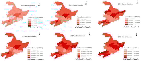
Figure 1.
Carbon Emissions statistics map of Northeast China in 2000, 2005, 2010, 2015, 2020, and 2022.
3.2. Variable Description
Based on previous studies and the literature, we have selected 16 driving factors related to carbon emissions, which are as follows:
- GDP [65]: Gross domestic product (GDP) measures the total value of economic activities within a given region. It is commonly used to assess economic development levels and the accumulation of social wealth.
- Proportion of the primary industry [66]: The share of agriculture, forestry, animal husbandry, and fishery in the GDP. A higher proportion often indicates a resource-dependent economy.
- Proportion of the secondary industry [66]: The share of industrial and construction sectors in the GDP. A higher proportion is typically linked to increased energy use and emissions.
- Proportion of the tertiary industry [66]: The share of the service sector in the GDP. An increasing share often signifies a transition to a lower-carbon, higher-value economy.
- Permanent population [67]: The permanent population refers to the total number of residents who have lived in a specific region for an extended period. Population size influences total energy consumption, infrastructure demand, and carbon emissions levels.
- Total energy consumption [68]: This indicator measures the total amount of energy consumed in a region for all economic activities and residential use.
- Coal consumption ratio [68]: This represents the proportion of coal in total energy consumption. Given that coal combustion releases substantial amounts of carbon dioxide (CO2) and pollutants such as sulfur dioxide (SO2) and nitrogen oxides (NOx), a higher coal consumption ratio is generally associated with increased carbon emissions and environmental degradation.
- Total electricity consumption [69]: This refers to the total power consumption of all sectors and residential users within a region, serving as an indicator of economic development and industrial energy demand.
- Urbanization rate [70]: This metric represents the proportion of the population residing in urban areas. Urbanization significantly impacts energy consumption, transportation patterns, infrastructure development, and carbon emissions.
- Proportion of fiscal expenditure on science and technology (R&D spending) [71]: The share of local government spending on scientific research and technological innovation. Higher investment can facilitate low-carbon technologies and improve energy efficiency.
- Dust emissions [72]: This refers to the total particulate matter emitted from industrial activities, primarily from coal-fired power plants, steel manufacturing, and cement production. This indicator directly affects air quality and environmental health.
- Green coverage rate in built-up areas [73]: This measures the proportion of green space within urban built-up areas. A higher green coverage ratio enhances carbon sequestration, mitigates the urban heat island effect, and improves air quality.
- Sulfur dioxide emissions [72]: SO2 is a major pollutant generated by coal combustion, smelting, and chemical production. Excessive SO2 emissions contribute to acid rain and air pollution, posing threats to ecosystems and public health.
- Average humidity [74]: This represents the average level of atmospheric moisture over a given period. Variations in humidity influence air quality, ecosystem stability, and climate adaptation.
- Precipitation [74]: This denotes the total volume of precipitation over a specified period, which directly affects regional water resource availability, ecosystem stability, and agricultural productivity.
- Average temperature [74]: This refers to the mean temperature over a given period, which is significantly influenced by global climate change and can impact regional energy demand, agricultural production, and ecosystem dynamics.
4. Methodology
4.1. Feature Selection
Before using machine learning methods for regression prediction, feature selection is the first step, which is also referred to as feature engineering in some studies [75]. Feature selection is a critical process that helps identify the features in the raw data that significantly influence the prediction outcomes, while eliminating redundant or irrelevant features. This reduces the complexity of the model, enhances its training efficiency, and improves its predictive performance. By performing feature selection, we can not only increase the accuracy of the model but reduce the risk of overfitting and improve the generalization capability of the model.
4.1.1. Correlation Analysis
Correlation analysis is a statistical method used to evaluate the linear relationship between two or more variables. It helps to understand the dependencies between features, which is crucial for feature selection and model design. The most commonly used measure of correlation is the Pearson correlation coefficient [76], which quantifies the degree of linear association between two variables. In this study, correlation analysis not only facilitates the identification of linear associations between various auxiliary variables and carbon emissions but assists in screening out key variables with significant impacts on carbon emissions. Furthermore, it provides a clear understanding of the intensity and direction of interactions between auxiliary variables, enabling the quantification of their linear associations. This method thus offers a scientific foundation for feature selection and model design, enhancing the accuracy and robustness of the research. The formula for the Pearson correlation coefficient is as follows:
where is the Pearson correlation coefficient; and are the observed values of variables and , respectively; and are the mean values of variables and , respectively; is the number of data points.
The value of the Pearson correlation coefficient ranges from −1 to 1: 1 indicates a perfect positive correlation, meaning that, as increases, also increases; −1 indicates a perfect negative correlation, meaning that, as increases, decreases; 0 indicates no linear relationship.
4.1.2. Multicollinearity Testing
Multicollinearity Testing is an important step in regression analysis to evaluate whether there is a high correlation between independent variables. High multicollinearity can lead to unstable regression coefficients, affecting the model’s predictive ability and interpretability. A common method for testing multicollinearity is the variance inflation factor (VIF) [77], which quantifies the linear dependence between each independent variable and the others. Each independent variable has an associated VIF value, and a higher VIF indicates stronger multicollinearity with other variables. The formula for calculating VIF is as follows:
where is the variance inflation factor for the -th variable, is the coefficient of determination when the -th variable is regressed on all other variables. = 1: no multicollinearity, indicating that the variable is independent of the others; 1 < < 10: moderate multicollinearity, which is generally not problematic. A value of > 10 indicates severe multicollinearity, suggesting the need for remediation.
Multicollinearity testing helps us identify and select independent variables that exhibit a high degree of correlation, thereby avoiding instability in regression coefficients caused by redundant variables. This ensures the independence of each independent variable within the model, enhancing the interpretability of the coefficients and improving the model’s predictive capabilities. Furthermore, multicollinearity testing promotes a deeper understanding of the relationships among independent variables. By analyzing VIF values, we can identify variables that may exhibit synergistic effects in explaining the changes in carbon emissions. This understanding is critical for formulating targeted policy recommendations. For instance, if two auxiliary variables demonstrate a relatively high VIF, we may advise the consideration of both factors in emissions reduction policies to achieve a more comprehensive approach to addressing carbon emissions.
4.2. Machine Learning Algorithm
With the rapid development of machine learning in recent years, its applications in predictive regression tasks have become increasingly widespread. This study compares the performance of several regression methods, including support vector machine (SVM), K-nearest neighbors (KNN), random forest, eXtreme Gradient Boosting (XGBoost), ridge regression, and lasso regression, based on data from 35 cities in Northeast China over the period from year 2000 to 2023. Building on this comparison, a stacking model was developed and its predictive performance was evaluated.
4.2.1. Support Vector Machine (SVM)
A support vector machine (SVM) is a powerful supervised learning method widely applied in both classification and regression tasks. The core idea of the SVM is to find an optimal hyperplane that separates data from different classes while maximizing the margin between them. In regression tasks, the goal of the SVM is to find an optimal hyperplane that not only fits the training data well but has good generalization ability.
We have training data points, where is the input feature (auxiliary variables such as GDP, population, and others) and is the target variable (carbon emissions). The goal of the SVM is to find a hyperplane, represented as follows:
where is the normal vector to the hyperplane, is the bias term, and is the input feature vector.
The loss function can be calculated as follows:
where is the hinge loss function, is the tolerance, are the slack variables, is the regularization parameter.
The optimization problem can be formulated as follows:
where C is the penalty parameter that controls the tolerance for errors.
4.2.2. K-Nearest Neighbors (KNN)
The K-nearest neighbors (KNN) is a simple yet powerful supervised learning algorithm, widely used for classification and regression tasks. The core idea of the KNN algorithm is to select the K most similar neighbors for a new input sample based on the distance between the new sample and the training samples, in order to perform classification or regression.
The Euclidean distance can be calculated as follows:
where is the new sample, is the training sample, is the -th feature, is the number of features (dimensionality).
4.2.3. Random Forest
Random forest is a powerful ensemble learning algorithm commonly used for classification and regression tasks. In a regression task, random forest predicts continuous values by combining multiple decision trees. Each tree is trained using a different subset of training data and considers only a random subset of features. During prediction, random forest aggregates the predicted results from each tree to make the final prediction.
Multiple subsets of the original training dataset are randomly generated using bootstrapping (sampling with replacement). Each subset is used to train an independent decision tree. Each decision tree is trained on its own data subset. The features at each node are chosen randomly from a subset of the available features, not from all features. For regression tasks, each tree provides a prediction. The final prediction from the random forest is the average of the predictions made by all the trees. The final regression prediction is the average of all the tree predictions:
where represent the total number of trees, and is the prediction made by the -th tree.
4.2.4. eXtreme Gradient Boosting (XGBoost)
XGBoost is an efficient and scalable implementation of gradient boosting, a machine learning technique for both regression and classification tasks. It builds an ensemble of decision trees sequentially, where each tree corrects the errors made by the previous one.
In gradient boosting, each tree is added to the model sequentially, with each tree aiming to minimize the residual errors (i.e., the difference between the predicted and actual values) from the previous model. The process iterates, and trees are added one by one, refining the predictions. XGBoost includes L1 and L2 regularization terms, which help to control overfitting and improve the generalization of the model. The regularization term is added to the objective function, making the optimization process more robust. The objective function in XGBoost is as follows:
where is the loss function, is the regularization term for the -th tree, represents the model parameters, represents the tree model, and , where is the number of leaves and is the weight of leaf
4.2.5. Ridge Regression
Ridge regression is a variant of linear regression that is primarily used to address multicollinearity in linear regression models. Ridge regression adds a regularization term to the ordinary least squares (OLS) loss function to penalize large regression coefficients, thereby reducing model complexity and preventing overfitting. This results in the following objective function:
where is the ordinary least squares loss, is the regularization term, with controlling the strength of the penalty. A larger increases the penalty on the coefficients, while a smaller allows for less regularization.
4.2.6. Lasso Regression
Lasso regression (least absolute shrinkage and selection operator) is another variant of linear regression that, like ridge regression, adds a regularization term to the loss function. However, instead of penalizing the square of the coefficients (as in ridge), lasso uses the absolute value of the coefficients. This leads to some coefficients being exactly zero, effectively performing feature selection by eliminating unimportant variables. The objective function for lasso regression is as follows:
where is the ordinary least squares loss, is the regularization term, and controls the strength of the penalty. A larger leads to more coefficients shrinking to zero, while a smaller allows the coefficients to be closer to their OLS estimates.
4.2.7. Stacking Regressor
Stacking, a widely-used ensemble learning method, has proven to be effective in improving predictive accuracy by combining multiple models. In the context of regression tasks, the stacking regressor leverages the predictions from multiple base learners and feeds these outputs into a meta-model, which makes the final prediction. This approach takes advantage of the strengths of individual models and combines them to achieve superior generalization capabilities. This paper discusses the application of a stacking regressor using random forest and XGBoost as base learners and a support vector machine (SVM) as the meta-model.
In regression tasks, random forest is an ensemble method based on bagging, which reduces noise interference by averaging the predictions of multiple decision trees, thereby enhancing model stability. XGBoost, on the other hand, is a gradient boosting decision tree algorithm based on boosting. It incorporates regularization and handles missing values effectively, thus mitigating the risk of overfitting. Additionally, it demonstrates strong computational efficiency and scalability. These two methods exhibit distinct advantages in regression tasks and represent two different ensemble strategies. Consequently, their combination captures diverse features and patterns in the data, thereby reducing the bias and variance associated with individual models.
For the meta-model in our stacking framework, we have selected the support vector machine (SVM). The SVM excels in regression tasks, particularly through the application of the kernel trick, which enables the effective handling of high-dimensional data and nonlinear relationships. In the context of stacking, the first stage typically generates predictions from multiple base models. These predictions can be regarded as high-dimensional features input to the meta-model. With its global optimization capability, the SVM identifies complex pattern combinations within these high-dimensional features, thereby producing an optimal prediction, and further enhancing the overall model’s accuracy. By contrast, linear regression, a commonly used meta-model, assumes a linear relationship between features and the target variable. When the input features consist of predictions from multiple base models, the intricate interactions between these models and the nonlinear predictive combinations may lead to suboptimal performance, as linear regression is not well-suited to capture such complexities.
Base learners (Level-0): The random forest regressor utilizes an ensemble of decision trees to predict the target variable. The XGBoost regressor implements a gradient boosting framework, combining weak learners (decision trees) in an additive fashion to reduce prediction errors.
Meta-Model (Level-1): The outputs of the base learners serve as new features for a meta-model. In this case, an SVM model is trained to predict the final output. The SVM learns to combine the predictions of the base learners and adjust the final prediction accordingly. The model architecture diagram is shown in Figure 2. The following explains in detail how the outputs from one stage serve as inputs for the subsequent stage:

Figure 2.
Stacking Model Architecture Diagram.
Each base learner (random forest and XGBoost) generates independent predictions. A training dataset , where represents the feature vector of the -th sample and represents the target variable, the predictions from the base learners are computed as follows:
where and are the prediction functions of the fandom forest and XGBoost models. These predicted values become the inputs for the next stage, which is the meta-model. Specifically, the predictions () from the base learners serve as new features for the meta-model.
The predictions from the base learners are combined into a new feature matrix , the meta-model (SVM) uses this new feature matrix as input to predict the final output as follows:
The final prediction for the -th sample is given by the following:
4.3. Model Description and Evaluation
4.3.1. Model Description
Before training and predicting with the model, it is essential to properly set the input parameters to ensure that the model can effectively fit the training data while maintaining good generalization ability, thus preventing issues such as overfitting and underfitting. The dataset is divided reasonably, with 80% allocated for the training set and the remaining 20% for the test set. At the same time, we used a five-fold cross-validation to evaluate the models and applied grid search to optimize the hyperparameters. The best parameter settings for each model are presented in Table 2.
Table 2.
Model description.
4.3.2. Performance Evaluation
For the evaluation of the aforementioned models, we employ the following metrics to assess the performance and accuracy of the predictions, which help us to quantify how well the model fits the data and how accurately it predicts outcomes:
R-squared (): This statistic measures the proportion of variance in the dependent variable that is explained by the independent variables. A higher value indicates a better fit of the model to the data.
where denotes the actual value, represents the predicted value, and is the mean of the actual values.
Mean Squared Error (MSE): MSE is the average of the squared differences between the actual and predicted values. It is a measure of how close the predictions are to the actual outcomes. A lower MSE indicates better model performance, as it means the predicted values are closer to the true values.
where denotes the actual value, represents the predicted value, and is the number of observations.
Mean Absolute Error (MAE): MAE calculates the average of the absolute differences between the actual and predicted values. It gives an idea of the magnitude of the errors in a model without considering their direction. Like MSE, a lower MAE indicates better model accuracy, but MAE is less sensitive to large errors compared to MSE.
where denotes the actual value, represents the predicted value, and is the number of observations.
4.4. Feature Importance
For evaluating the contribution of each auxiliary variable to carbon emissions, traditional feature importance methods are typically directly generated by machine learning algorithms. For example, tree-based models (such as random forest and XGBoost) assess the importance of each feature by calculating the average reduction in impurity (such as information gain or Gini index) [78,79]. However, these methods may fail to effectively capture complex interactions between features, especially in scenarios where nonlinear relationships and feature interactions are strong.
Based on the stacking model, we use SHAP values to quantify the contribution of each auxiliary variable to carbon emissions, and derive a ranking of these contribution values. SHAP (Shapley additive explanations) values [80] are a tool used to interpret the predictions of machine learning models, derived from the Shapley value in game theory. The core idea is to calculate the “fair” contribution of each feature to the model’s prediction, thereby measuring the importance of each feature. Compared to traditional feature importance methods, SHAP values not only measure the individual impact of each feature but capture the interactions between features, which is particularly important for complex machine learning models. In this study, a SHAP analysis precisely shows the specific contribution of each variable to carbon emissions prediction, and reveals potential nonlinear and interaction effects between these variables (such as GDP, total energy consumption, etc.). This interpretability not only aids in understanding the prediction mechanisms of the model but provides strong support for policymakers to formulate effective emissions reduction strategies. By identifying the most influential factors, decision-makers can adopt more targeted measures, enhancing the implementation outcomes of policies.
For a given sample, the prediction value is first calculated without considering a specific feature. Then, each feature is sequentially added, and the prediction value increment after adding that feature is calculated. Afterward, all possible combinations of features are considered, and the incremental contributions for each combination are averaged with weights to obtain the Shapley value for each feature. The formula for the Shapley value is as follows:
where is the Shapley value of feature , representing the contribution of feature to the prediction result, is the set of all features, is a subset of features, represents the prediction value when the feature set is , is the prediction value, is the sizes of the subset and the feature set, respectively.
4.5. Scenario Simulation
Step 1: Based on the SHAP importance rankings, and considering the characteristics of heavy industry and climate conditions in Northeast China, we selected total energy consumption, urbanization rate, coal consumption ratio, GDP, and average temperature as core regulatory variables. It is important to note that the chosen growth rates are based on current assumptions and observed trends. These assumptions and trends are primarily derived from past economic growth patterns, energy consumption structures, and historical climate data. However, these assumptions may be influenced by unforeseen events, which could alter the simulation results. For example, the COVID-19 pandemic that erupted in 2019 had a profound impact on the global economy and energy consumption, with lockdown measures causing many economic activities to be paused, subsequently affecting the growth rates of related variables [81]. Therefore, the growth rates used in our simulation assume that no unforeseen events will occur in the future and do not guarantee full adaptation to similar unexpected events or policy changes. Three typical pathways are designed as follows: the “Baseline Scenario”, the “Aggressive De-coal Scenario”, and the “Climate Resilience Scenario”. These scenarios quantify the threshold values for the average annual change rates of each variable.
- Baseline Scenario (BS): This scenario represents the future development path under current policies and trends, without significant adjustments to the existing energy consumption structure, economic growth model, or climate change mitigation efforts. It typically represents a “business-as-usual” situation, characterized by a lack of major policy changes. The annual change rates for the variables—energy consumption, urbanization rate, coal consumption ratio, GDP, and average temperature—are set at 2%, 1%, −1%, 2%, and 0.4%, respectively.
- Aggressive De-coal Scenario (ADS): This scenario assumes more aggressive policy measures in the future to reduce coal dependence and lower carbon emissions. It involves significantly reducing coal usage and accelerating the energy structure transition, such as increasing the use of renewable energy and improving energy efficiency. The annual change rates for the variables—energy consumption, urbanization rate, coal consumption ratio, GDP, and average temperature—are set at 1%, 2%, −3%, 3%, and 0.8%, respectively.
- Climate Resilience Scenario (CRS): This scenario focuses on enhancing society’s ability to adapt to and build resilience against climate change, while promoting energy consumption and urbanization. It aims to control greenhouse gas emissions through strategies such as improving energy efficiency, increasing the use of renewable energy, and strengthening climate change adaptation strategies. The annual change rates for the variables—energy consumption, urbanization rate, coal consumption ratio, GDP, and average temperature—are set at 5%, 4%, 0%, 7%, and 0.2%, respectively.
Step 2: Constructing the Policy–Energy–Climate Model. This model is used to simulate the changes in carbon emissions under different policy scenarios. In each scenario, the input features will be adjusted according to the preset change rates. The specific formula is as follows:
where represents the original data, and refers to the rate of change in the scenario.
Step 3: Monte Carlo Simulation
A Monte Carlo simulation is a statistical method that involves performing multiple experiments through random sampling. Based on statistical principles, it estimates system properties by repeatedly sampling randomly, making it particularly suitable for complex systems involving multiple interacting factors. In this paper, we use the Monte Carlo simulation to model the temporal variation and scale of carbon emissions peak timing and peak levels under different scenarios, providing a probability distribution for assessing future carbon emissions. In each scenario, future carbon emissions data are simulated by applying different rates of change, and a stacking model is used for predictions. By conducting 3000 simulations, the distribution of peak timing and peak levels for each scenario is obtained. This number was determined based on a trade-off between computational efficiency and result stability, ensuring minimal variation in the results, while accurately representing the potential probability distribution. The mean and standard deviation of the peak timing and peak levels are calculated to assess the uncertainty of carbon emissions under different scenarios. The mean provides a median estimate of the peak timing and peak levels, while the standard deviation reflects the dispersion of the results, describing the range of possible outcomes. The Monte Carlo simulation not only provides a rigorous quantitative estimate of carbon emissions peak but deepens the understanding of result uncertainty through a probabilistic framework, thereby providing important insights for a more informed climate change policy development.
5. Results and Discussion
5.1. Results of Feature Selection
The bubble heatmap of the correlation matrix is shown in Figure 3, providing a visual representation of the pairwise correlations between all the remaining selected features. In the figure, the transition from green to yellow represents an increasing positive correlation, while the transition from green to purple indicates an increasing negative correlation. The size of the bubbles corresponds to the strength of the correlation; larger bubbles indicate stronger correlations, while smaller bubbles suggest weaker correlations.
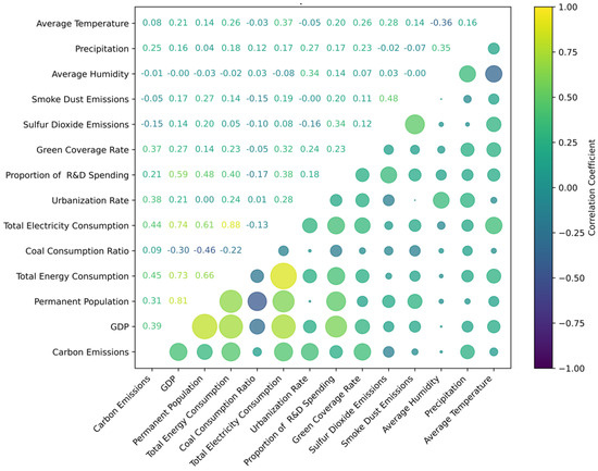
Figure 3.
Bubble Heatmap of Correlation Matrix.
Based on the analysis of the correlation heatmap, we found that variables such as GDP, permanent population, total energy consumption, total electricity consumption, and urbanization rate exhibit a high positive correlation with carbon emissions, with correlation coefficients of 0.39, 0.31, 0.45, 0.44, and 0.38, respectively. This result aligns with logical expectations, as higher economic activity (GDP), increased population, and greater energy consumption typically lead to higher carbon emissions due to the direct energy usage and industrial activities associated with these factors. Additionally, urbanization often results in more energy-intensive infrastructure and transportation, further contributing to carbon emissions. On the other hand, variables such as smoke dust emissions, sulfur dioxide emissions, and average humidity show a negative correlation with carbon emissions, with correlation coefficients of −0.05, −0.15, and −0.01, respectively. This suggests that these variables, while related to other environmental factors, do not directly contribute to the emissions of carbon.
Additionally, among the auxiliary variables, permanent population (0.81), total electricity consumption (0.74), and total energy consumption (0.73), as well as the correlation between total energy consumption and total electricity consumption (0.88) and permanent population (0.66), exhibit strong positive correlations. This is because GDP, population, electricity consumption, and energy consumption tend to influence each other, contributing to the overall economic and energy dynamics of the region. In more developed cities of various provinces, such as Harbin, in Heilongjiang Province, Shenyang and Dalian, in Liaoning Province, where there are larger populations, higher GDP, and more developed industries, this leads to higher energy and electricity consumption. However, further calculations are needed to determine whether multicollinearity exists, and whether any variables need to be excluded from the analysis.
In conducting the multicollinearity test, we used a variance inflation factor (VIF) value greater than 10 as the criterion for determining the presence of multicollinearity. If the VIF is greater than 10, it is considered to indicate multicollinearity. After the analysis, the three indicators for the proportion of the primary, secondary, and tertiary industries were excluded due to multicollinearity (VIF > 10). The VIF values for the remaining variables, along with descriptive statistics, are presented in Table 3. By analyzing the VIF values, we found that most variables have VIF values between 1 and 2. Among them, electricity consumption has the highest VIF value at 7.970, but it is still below the threshold of 10. Overall, all the variables have VIF values below the threshold of 10. These results suggest that, although there is some multicollinearity among the proportions of industrial sectors, the overall multicollinearity issue in the model is not severe.
Table 3.
Statistical description table with Variance Inflation Factor value.
In the descriptive statistics, we described the maximum, minimum, average, and standard deviation of each variable. Despite differences in units and scales, there is significant variation in these variables across different cities and years in Northeast China from 2000 to 2022. This also reflects the significant fluctuations in factors such as regional economic development, industrial structure, and energy consumption, as well as the imbalanced development of these variables over different time periods, showing dynamic differences across cities in these variables. Ultimately, we identified 13 driving factors of carbon emissions in Northeast China from four aspects: economics, energy, environment, and climate, as shown in Figure 4.

Figure 4.
Driving Factors of Carbon Emissions in Northeast China.
5.2. Regression of Carbon Emissions
In this study, we applied several machine learning algorithms to predict carbon emissions data from Northeast China, as discussed previously. The regression results from the first six individual models are presented in Figure 5, where the performance of each algorithm is illustrated in terms of their predictions on both the training and testing datasets. These models were selected for their established effectiveness in regression tasks, each having different approaches to capturing data patterns. By contrast, Figure 6 showcases the predictive performance of the novel stacking model proposed in this study. This hybrid model integrates random forest, XGBoost, and an SVM to leverage the strengths of each individual model, aiming to achieve improved predictive accuracy. The stacking approach allows for more robust predictions by combining the outputs of the base models and learning from their respective strengths and weaknesses.
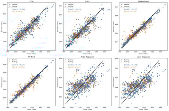
Figure 5.
Regression fitting of carbon emissions in Northeast China in different machine learning algorithms (Training data and Testing data).
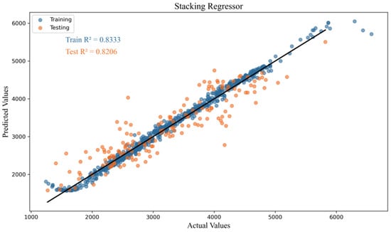
Figure 6.
Regression fitting of the novel stacking model.
To further evaluate the performance of the models, Table 4 presents the prediction results for various algorithms, including , MSE, and MAE. A detailed analysis of the evaluation metrics leads to the following conclusions: In the training set, the XGBoost model achieved the highest R2 value with 0.85, indicating that XGBoost provided the best fit during training. XGBoost demonstrated a strong ability to capture the patterns in the training data, highlighting its robust modeling capability for this dataset. However, in the test set, the newly proposed stacking model outperformed the others. This model, which combines the strengths of XGBoost and random forest, achieved an R2 value of 0.82, with the lowest MSE and MAE, indicating the superior generalization ability of the stacking model on the test data.
Table 4.
Comparison of prediction performance of different machine learning algorithms (, MSE, MAE with two decimal places, * represents the optimal value for each metric.
Overall, in this study, lasso and ridge regression, as simple variant regression methods, exhibited relatively poor fitting performance. The R2 values on both the training and test sets were below 0.5, as these methods have limited capacity to model the complex nonlinear relationships among features. This is especially evident in the context of the diverse and strongly nonlinear characteristics of the data in this study, where the linear assumptions of lasso and ridge constrained their performance. By contrast, ensemble learning methods, such as XGBoost and random forest, demonstrated superior performance for the problem at hand. Ensemble learning methods, by combining the predictions of multiple base models, effectively reduce the bias inherent in individual models and enhance overall predictive performance. Based on this, we designed a stacking model combining XGBoost and random forest, and the results clearly indicated its superior performance compared to the base models used individually. This stacking model fully leveraged the complementary strengths of XGBoost and RF, ultimately improving performance on the test set and demonstrating its strong predictive power in addressing the research problem.
5.3. Results of Feature Importance
Based on the stacking model and the SHAP method, we obtained the SHAP values and feature importance for each variable, as shown in Figure 7. In the SHAP value visualization, yellow represents higher feature values, while purple represents lower feature values. The yellow area on the positive axis indicates that the variable has a positive effect on carbon emissions, meaning that higher feature values lead to an increase in carbon emissions. By contrast, the yellow area on the negative axis indicates that the variable has a negative effect on carbon emissions, meaning that higher feature values lead to a decrease in carbon emissions. The Feature Importance chart, based on the mean absolute SHAP values (mean |SHAP value|), represents the average magnitude of each variable’s impact on the model’s output. This provides an indication of the relative importance of each feature.
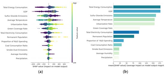
Figure 7.
SHAP value and Feature Importance: (a) the visualization shows the SHAP values for each variable, (b) represents the average magnitude of each variable’s impact on the model’s output.
Upon further analysis of Figure 7, we observe that variables such as total energy consumption, urbanization rate, electricity, permanent population, and coal consumption ratio have significant positive effects on carbon emissions in Northeast China. Specifically, as energy consumption increases, particularly the use of fossil fuels, carbon emissions tend to rise significantly. At the same time, the advancement of urbanization is often accompanied by the expansion of construction, transportation, and industrial sectors, all of which require more energy, especially traditional energy sources like coal, thus further driving the increase in carbon emissions. Furthermore, electricity production and consumption are major sources of carbon emissions, especially in regions reliant on coal-fired power generation. The growth in electricity demand directly leads to increased energy consumption, which in turn contributes to higher carbon emissions. The growth of the permanent population generally leads to higher energy demand, further exacerbating the rise in carbon emissions. Finally, the use of coal is particularly closely linked to carbon emissions. As a traditional high-carbon energy source, coal consumption directly contributes to the increase in carbon emissions. In summary, these factors play a significant role in the rise of carbon emissions in Northeast China, especially within an economy heavily reliant on traditional energy. Their growth directly drives the increase in carbon emissions levels. Therefore, in the future, effectively addressing carbon emissions will require reducing the negative impacts of these variables and optimizing the energy structure, which will be crucial goals.
Sulfur dioxide emissions, smoke dust emissions, average temperate, and average humidity have a significant negative effect on carbon emissions. This indicates that an increase in these variables typically leads to a reduction in carbon emissions levels. Specifically, sulfur dioxide and smoke dust emissions can drive the adoption of clean energy technologies and the enhancement of pollution control measures, indirectly contributing to a reduction in carbon emissions. The increase in temperature and humidity has a significant negative effect on carbon emissions, which warrants attention. Higher humidity and temperature may have a suppressive effect on energy consumption, particularly in energy-intensive regions such as Northeast China, where air conditioning and heating are common. In high-humidity environments, the increased water vapor content in the air reduces the demand for temperature regulation, which in turn helps to reduce energy consumption from air conditioning and heating, thus lowering carbon emissions. However, in low-humidity, high-temperature environments, the demand for air conditioning and heating systems increases significantly, leading to higher overall energy consumption and, consequently, an increase in carbon emissions. Furthermore, changes in temperature and humidity largely affect the concentration and diffusion patterns of air pollutants, especially in urban and industrialized areas. These changes can lead to the concentration or dilution of pollutants, indirectly influencing carbon emissions. This makes it an important factor to consider when studying carbon emissions in Northeast China, where such climate-related variables play a particularly significant role.
Notably, the results revealed that the green coverage Rate appeared somewhat ambiguous in the SHAP value plot, with some yellow regions in the positive area and others in the negative area. However, the overall trend still leaned towards the positive area, indicating a positive correlation between green coverage and carbon emissions. This result initially seems counterintuitive, but a closer analysis reveals that this phenomenon has its specificities in Northeast China. The increase in green coverage may be synchronized with the infrastructure construction in the rapid urbanization process. These areas may also experience higher energy consumption and industrial activities, leading to an increase in carbon emissions. Particularly during the warmer and colder seasons, the increased demand for air conditioning and heating could partially offset the carbon absorption effect of green coverage. Therefore, the negative correlation between green coverage and carbon emissions is actually a complex process that involves the net carbon absorption effect of vegetation, as well as the interaction with industrialization and energy consumption. In Northeast China, changes in green coverage represent not only an increase in carbon absorption but potential interactions with other socio-economic activities, which could complicate its impact on carbon emissions.
5.4. Results of Scenario Simulations
As shown in Figure 8, under different policy scenarios, the timing of the carbon peak exhibits significant variation across different cities. In both the Baseline Scenario (BS) and the Climate Resilience Scenario (CRS), the average carbon peak is expected around 2039–2040. In the CRS, despite the implementation of additional climate adaptation measures, such as improving societal resilience to climate change and enhancing energy efficiency, energy consumption and urbanization continue to grow. Although the scenario attempts to mitigate greenhouse gas emissions by increasing the use of renewable energy and boosting climate resilience, no fundamental changes are made to the energy structure or coal consumption. As a result, carbon emissions remain at relatively high levels, and this scenario, focused more on adaptation rather than emissions reduction, fails to significantly advance the carbon peak. By contrast, the Aggressive De-coal Scenario (ADS) anticipates the carbon peak in 2030, which is approximately ten years earlier than in the other two scenarios, and achieves the largest carbon emissions reduction (17.5–24.6%). This scenario assumes the adoption of more aggressive policies, particularly in reducing coal use and accelerating energy structure transformation. Through substantial increases in renewable energy use and improved energy efficiency, the proportion of coal consumption is significantly reduced. These measures effectively accelerate the decline in carbon emissions, leading to an earlier carbon peak. This scenario underscores the pivotal role of comprehensive policy adjustments in rapidly achieving a carbon peak and initiating a decline, highlighting the significant impact of aggressive de-coalization strategies on driving the transition to a low-carbon economy.
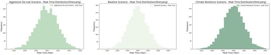

Figure 8.
Distribution of the Carbon Peak Time Under Different Scenarios (Shenyang, Changchun, Dalian, Harbin).
Table 5 presents the mean and standard deviation of carbon emissions at the carbon peak in different cities under various scenarios. An analysis reveals that, in all scenarios, the carbon peak emissions in each city are lower than those of the baseline year (2022), indicating that carbon emissions can be effectively controlled under any policy pathway, in line with the carbon peak target. This reflects the carbon reduction potential across different policy scenarios, and highlights the positive impact of policy measures in reducing carbon emissions. The differences in carbon peak emissions across the various scenarios are relatively small, suggesting that the carbon emissions levels are stable across different policy pathways, without significant fluctuations. This indicates that, while the policy paths differ, the impact of these scenarios on carbon emissions remains within expected ranges, demonstrating that policy adjustments may lead to different levels of emissions reductions, but the overall trend remains stable. Notably, the Aggressive De-coal Scenario (ADS) exhibits the lowest standard deviation, meaning that the carbon emissions in this scenario are more consistent, with stronger predictability. Compared to other scenarios, the ADS involves more substantial policy interventions, particularly in reducing coal use and accelerating energy structure transformation, which results in a more stable and controlled emissions reduction effect.
Table 5.
Mean and Standard Deviation of the Carbon Peak Emissions Under Different Scenarios (Shenyang, Changchun, Dalian, Harbin).
To facilitate a direct comparison of the three scenarios and to highlight the policy trade-offs, Table 6 summarizes the key parameter settings, the projected carbon peak times, and concise policy implications for each scenario.
Table 6.
Comparative Summary of Scenario Parameters, Projected Peak Times, and Policy Implications.
As shown in Table 6, the Aggressive De-coal Scenario (ADS) is the only pathway that achieves the carbon peak by 2030, aligning with China’s national target. However, this scenario requires the most significant policy interventions and may entail short-term economic adjustments. The Baseline Scenario (BS) and Climate Resilience Scenario (CRS), while less disruptive in the short term, delay the carbon peak to around 2039–2040, underscoring the need for more ambitious emissions reduction efforts.
In summary, although the overall results of the scenario simulations indicate that the Aggressive De-coal Scenario (ADS) performs better in terms of carbon peak achievement for several cities in Northeast China, with an earlier peak time and smaller standard deviation of carbon emissions, suggesting more stable and predictable carbon reduction effects, we should critically assess this aggressive policy path. While the strong de-coalization policy can rapidly reduce carbon emissions and accelerate the achievement of the carbon peak in the short term, its negative impacts on the environment, society, and economic development cannot be overlooked. Particularly in the short term, an over-reliance on reducing coal consumption may exert pressure on energy supply, industrial transformation, employment, and economic growth, potentially leading to higher energy prices and social instability. Specifically, employment shifts in coal-dependent industries could lead to significant job losses, posing challenges to social stability and economic development. Furthermore, overly aggressive energy structural adjustments may fail to fully account for the economic feasibility and actual resource endowments of local areas, resulting in significant economic losses and social adaptation challenges during the transition period. Therefore, it is essential to carefully assess the economic feasibility of such policies and implement effective measures to address the employment transition challenges.
Based on the above results, and considering the unique geographical, climatic, and energy characteristics of Northeast China, we have formulated specific policy recommendations for each scenario to achieve carbon neutrality and peak carbon emissions.
Baseline Scenario: Under the Baseline Scenario, prioritize strengthening existing energy efficiency standards. Gradually increase renewable energy use, focusing on readily available sources. Enhance carbon emissions monitoring and data collection to track progress and identify further improvement areas. This is a measured, incremental approach.
Aggressive De-coal Scenario: The Aggressive De-coal Scenario requires strict coal regulations, potentially including carbon taxes. Massively deploy renewables with incentives and streamline permitting. Invest in smart grids and energy storage. Provide “Just Transition” support for affected workers and communities. Promote carbon capture, utilization, and storage (CCUS) technologies to mitigate CO2 emissions from hard-to-decarbonize sectors.
Climate Resilience Scenario: The Climate Resilience Scenario focuses on climate-proofing infrastructure and promoting climate-resilient agriculture. Enhance natural carbon sequestration through afforestation and wetland restoration. Encourage moderate energy efficiency improvements in buildings and industry. This balances emissions reductions with climate adaptation.
5.5. Policy Recommendations
Based on the conclusions drawn in Section 5.3 and Section 5.4, and taking into account the unique geographical, climatic, and energy characteristics of Northeast China, the following four targeted policy recommendations are proposed to achieve carbon neutrality and the carbon peak goals.
Accelerating Energy Transition and Promoting Clean Energy Development: Northeast China’s coal-dependent steel, chemical, and power industries drive high emissions, exacerbated by severe winters. Reducing coal reliance requires expanding wind, solar, and biomass energy in Liaodong Peninsula and the Songnen Plain. Smart grids and energy storage should enhance renewable energy integration and stabilize winter power. Clean coal technologies and CCUS must be promoted. Government subsidies and tax incentives should support industrial parks in adopting renewable energy and optimizing power distribution.
Facilitating Low-Carbon Transition of High-Energy-Intensive Industries: Northeast China’s steel, petrochemical, and cement sectors need rapid low-carbon transition. Hydrogen metallurgy and CCUS should be prioritized. Industrial restructuring must shift toward high-end manufacturing and clean energy vehicles. A carbon trading market should increase costs for high-emissions industries, driving efficiency. Circular economy industrial parks should enhance waste utilization. Green finance mechanisms should incentivize investment in carbon reduction technologies.
Promoting Green Urbanization and Enhancing Energy Efficiency: Northeast China’s urbanization intensifies building and transportation emissions. Green construction and energy-efficient retrofitting should be implemented, incorporating insulation materials, geothermal energy, and air-source heat pumps. Electric buses, rail transit, and shared mobility should be prioritized. Charging and hydrogen refueling stations must expand to support electric and hydrogen-powered vehicles.
Enhancing Carbon Sequestration and Promoting Low-Carbon Agriculture: Northeast China’s forests, wetlands, and black soil are vital carbon sinks but face deforestation and degradation. Afforestation and sustainable forest management should improve carbon storage. Low-carbon agriculture, including organic fertilization and optimized irrigation, should enhance soil sequestration. Wetland restoration programs must reinforce carbon sinks. Carbon trading mechanisms should encourage reforestation and conservation investment, aligning ecology with economic benefits.
Mitigating Economic and Social Impacts of De-coalization: To mitigate the economic and social impacts of the Aggressive De-coal Scenario (ADS), and to ensure a just transition, a phased and integrated approach is needed. Initially, a regional “Just Transition Fund” should be established to provide immediate support to affected workers, communities, and businesses. Concurrently, financial incentives should be implemented to stimulate investment in renewable energy and energy efficiency. As these investments take effect, retraining programs become crucial for displaced workers, coupled with unemployment benefits and relocation assistance to facilitate their transition. To ensure long-term sustainability, economic diversification is essential, fostering new industries like renewable energy manufacturing and green technology; this requires supportive infrastructure and targeted assistance for SMEs.
By implementing these policy measures, Northeast China can effectively reduce carbon emissions while maintaining economic development, thus contributing to achieving national carbon neutrality and carbon peak objectives. Considering the region’s specific energy structure and climatic conditions, these recommendations provide a robust framework for long-term sustainable development.
6. Conclusions
This study applies a machine learning-based stacking model to analyze carbon emissions in Northeast China, integrating prediction, factor interpretation, and policy simulation. By developing a stacking model with random forest and XGBoost as base learners and a support vector machine (SVM) as the meta-model, the prediction accuracy was significantly improved, achieving an R2 of 0.82 on the test set, which outperforms several other machine learning models in terms of performance. The SHAP method was employed to quantify the contribution of key factors, yielding the average magnitude of each variable’s impact. Among these, total energy consumption and GDP exhibit the highest positive correlation, reaching 175, and are identified as the primary drivers of carbon emissions. By contrast, sulfur dioxide emissions and average temperature show significant negative correlations, with values around 150. A notable finding is the positive correlation between green coverage and carbon emissions in Northeast China, which is attributed to the complex interplay of various factors, including climate, social, and economic influences. Scenario simulations indicate that, under the Aggressive De-coal Scenario (ADS), Northeast China is expected to reach peak carbon emissions by 2030, aligning with national targets. However, in the Baseline Scenario (BS) and Climate Resilience Scenario (CRS), the carbon peak occurs around 2039–2040, highlighting the necessity of stringent policy interventions. In terms of the carbon peak levels, the ADS exhibits the smallest standard deviation, with values consistently around 5, whereas the BS and CRS scenarios show standard deviations around 10. This indicates that the simulation of carbon peak emissions under the ADS is more stable, with smaller fluctuations.
While focused on Northeast China, this study’s methodology offers broader applicability. The machine learning stacking approach can be adapted to analyze carbon emissions drivers and predict trends in other regions, provided appropriate data are available. The policy scenarios, particularly those emphasizing de-coalization and energy transition, provide insights for regions reliant on fossil fuels. However, direct application requires considering region-specific socio-economic and environmental contexts, including industrial structure, energy resources, and climate. Future research should explore the model’s transferability to other heavy industrial regions in China, particularly those with characteristics similar to the Northeast, validating and refining the model with their specific data and policy contexts. Concurrently, enhancing the model by incorporating real-time energy data (production, consumption, grid stability, emissions) is crucial for improved accuracy and decision support. This would enable dynamic adjustments to the ADS as the transition progresses. Granular socioeconomic impact assessments are also crucial, examining the effects on diverse demographic groups and communities, including quantitative analyses of job creation in green industries and qualitative studies of social and cultural impacts. Comparative analyses with other regions undergoing de-coalization could provide valuable best practices. Finally, investigating optimal financial policies to mitigate economic burdens, and exploring the role of emerging green technologies are essential for a successful and sustainable energy future.
Despite these contributions, this study has limitations. Firstly, the model used relies on historical data, which means it does not fully account for technological advancements and economic shifts, factors that may influence future carbon emissions trends. Future research should consider incorporating dynamic economic indicators and technological innovations into the model to enhance its adaptability and accuracy. Secondly, this study did not fully explore the spatial heterogeneity of emissions reduction potential across different cities. Future research could further improve the model’s robustness and broad applicability by conducting a multi-regional comparative analysis. Additionally, while the current machine learning model performs well in terms of prediction accuracy, the integration of deep learning methods could further improve the model’s forecasting precision and ability to handle complex data. Finally, while Monte Carlo simulations provide valuable scenario analysis, their assumptions regarding parameters might be overly simplified. For instance, the model assumes that key parameters remain stable across different scenarios, without fully considering extreme conditions or unforeseen events, such as economic crises or policy changes, which could lead to deviations from actual outcomes. Therefore, future research could introduce more uncertainties and random variables into Monte Carlo simulations to further enhance their realism and reliability. Overall, this study provides a data-driven approach for understanding carbon emissions trends in Northeast China and offers actionable policy recommendations. The findings support the region’s transition towards carbon neutrality and contribute to the broader goal of achieving China’s dual-carbon targets in a timely and sustainable manner.
Author Contributions
Conceptualization, X.R. and N.W.; methodology, X.R. and J.Z.; software, X.R. and J.Z.; validation, X.R., J.Z., and S.W.; formal analysis, X.R., J.Z. and S.W.; investigation, X.R.; resources, X.R., C.Z. and H.Z.; data curation, X.R., C.Z. and H.Z.; writing—original draft preparation, X.R.; writing—review and editing, S.W., C.Z., H.Z. and N.W.; visualization, X.R. and J.Z.; supervision, N.W.; project administration, N.W.; funding acquisition, N.W. All authors have read and agreed to the published version of the manuscript.
Funding
This study is supported by National Key R&D Program of China (2022YFC3702500), the National Higher Education Science Research Project (Key Project) of China Higher Education Association 2024 “Research on the Improvement of Teaching Content Reconstruction Ability Based on Multisource Online Teaching Material Comparison and LLM Assistance” (No. 24LK0305), Jilin University Special Project for Undergraduate Education and Teaching Reform Empowered by Artificial Intelligence (No. 24AI046Y), Jinan University—“Challenge Cup” and extracurricular academic, scientific, technological innovation, and entrepreneurship competition projects (Grant No. 20242020), the Special Funds for Cultivation of Guangdong College Students’Scientific and Technological Innovation (“Climbing Program” Special Funds).
Data Availability Statement
Data will be made available on request.
Conflicts of Interest
The authors declare that they have no known competing financial interests or personal relationships that could have appeared to influence the work reported in this paper.
References
- Li, R.; Wang, Q.; Liu, Y.; Jiang, R. Per-capita carbon emissions in 147 countries: The effect of economic, energy, social, and trade structural changes. Sustain. Prod. Consum. 2021, 27, 1149–1164. [Google Scholar] [CrossRef]
- Khan, I.; Hou, F.; Le, H.P. The impact of natural resources, energy consumption, and population growth on environmental quality: Fresh evidence from the United States of America. Sci. Total Environ. 2021, 754, 142222. [Google Scholar] [CrossRef]
- Zhao, X.; Ma, X.; Chen, B.; Shang, Y.; Song, M. Challenges toward carbon neutrality in China: Strategies and countermeasures. Resour. Conserv. Recycl. 2022, 176, 105959. [Google Scholar] [CrossRef]
- Osman, A.I.; Chen, L.; Yang, M.; Msigwa, G.; Farghali, M.; Fawzy, S.; Rooney, D.W.; Yap, P.S. Cost, environmental impact, and resilience of renewable energy under a changing climate: A review. Environ. Chem. Lett. 2023, 21, 741–764. [Google Scholar] [CrossRef]
- Amin, M.; Shah, H.H.; Fareed, A.G.; Khan, W.U.; Chung, E.; Zia, A.; Rahman Farooqi, Z.U.; Lee, C. Hydrogen production through renewable and non-renewable energy processes and their impact on climate change. Int. J. Hydrogen Energy 2022, 47, 33112–33134. [Google Scholar] [CrossRef]
- Dong, F.; Li, Y.; Gao, Y.; Zhu, J.; Qin, C.; Zhang, X. Energy transition and carbon neutrality: Exploring the non-linear impact of renewable energy development on carbon emission efficiency in developed countries. Resour. Conserv. Recycl. 2022, 177, 106002. [Google Scholar] [CrossRef]
- Ou, Y.N.; Iyer, G.; Clarke, L.; Edmonds, J.; Fawcett, A.A.; Hultman, N.; McFarland, J.R.; Binsted, M.; Cui, R.; Fyson, C.; et al. Can updated climate pledges limit warming well below 2 °C?; Increased ambition and implementation are essential. Science 2021, 374, 693–695. [Google Scholar] [CrossRef]
- Zhou, W.; Fan, W.; Lan, R.; Su, W.; Fan, J.L. Retrofitted CCS technologies enhance economy, security, and equity in achieving carbon zero in power sector. Appl. Energy 2025, 378, 124803. [Google Scholar] [CrossRef]
- Chen, L.; Msigwa, G.; Yang, M.; Osman, A.I.; Fawzy, S.; Rooney, D.W.; Yap, P.-S. Strategies to achieve a carbon neutral society: A review. Environ. Chem. Lett. 2022, 20, 2277–2310. [Google Scholar] [CrossRef]
- Meinshausen, M.; Lewis, J.; McGlade, C.; Gütschow, J.; Nicholls, Z.; Burdon, R.; Cozzi, L.; Hackmann, B. Realization of Paris Agreement pledges may limit warming just below 2 °C. Nature 2022, 604, 304–309. [Google Scholar] [CrossRef]
- Abbasi, K.R.; Shahbaz, M.; Zhang, J.; Irfan, M.; Alvarado, R. Analyze the environmental sustainability factors of China: The role of fossil fuel energy and renewable energy. Renew. Energy 2022, 187, 390–402. [Google Scholar] [CrossRef]
- Larsen, K.; Pitt, H.; Grant, M.; Houser, T. China’s greenhouse gas emissions exceeded the developed world for the first time in 2019. Rhodium Group, 6 May 2021. [Google Scholar]
- Liu, L.; Chen, C.; Zhao, Y.; Zhao, E. China׳ s carbon-emissions trading: Overview, challenges and future. Renew. Sustain. Energy Rev. 2015, 49, 254–266. [Google Scholar] [CrossRef]
- Huang, R.; Zhang, S.; Wang, P. Key areas and pathways for carbon emissions reduction in Beijing for the “Dual Carbon” targets. Energy Policy 2022, 164, 112873. [Google Scholar] [CrossRef]
- Zou, C.; Xue, H.; Xiong, B.; Zhang, G.; Pan, S.; Jia, C.; Wang, Y.; Ma, F.; Sun, Q.; Guan, C. Connotation, innovation and vision of “carbon neutrality”. Nat. Gas Ind. B 2021, 8, 523–537. [Google Scholar] [CrossRef]
- Hao, J.; Gao, F.; Fang, X.; Nong, X.; Zhang, Y.; Hong, F. Multi-factor decomposition and multi-scenario prediction decoupling analysis of China’s carbon emission under dual carbon goal. Sci. Total Environ. 2022, 841, 156788. [Google Scholar] [CrossRef]
- Dong, F.; Li, X.; Long, R.; Liu, X. Regional carbon emission performance in China according to a stochastic frontier model. Renew. Sustain. Energy Rev. 2013, 28, 525–530. [Google Scholar] [CrossRef]
- Wang, K.; Wu, M.; Sun, Y.; Shi, X.; Sun, A.; Zhang, P. Resource abundance, industrial structure, and regional carbon emissions efficiency in China. Resour. Policy 2019, 60, 203–214. [Google Scholar] [CrossRef]
- Yuan, D.; Dong, J. Research on ecological restoration and its impact on society in coal resource-based areas: Lessons from the Ruhr area in Germany and the Liulin area in China. Geoforum 2024, 154, 104038. [Google Scholar] [CrossRef]
- Dimanchev, E.G.; Paltsev, S.; Yuan, M.; Rothenberg, D.; Tessum, C.W.; Marshall, J.D.; Selin, N.E. Health co-benefits of sub-national renewable energy policy in the US. Environ. Res. Lett. 2019, 14, 085012. [Google Scholar] [CrossRef]
- Gao, Z.; Li, S.; Cao, X.; Li, Y. Carbon emission intensity characteristics and spatial spillover effects in counties in northeast China: Based on a spatial econometric model. Land 2022, 11, 753. [Google Scholar] [CrossRef]
- Cheng, H.; Dong, S.; Li, F.; Yang, Y.; Li, S.; Li, Y. Multiregional input-output analysis of spatial-temporal evolution driving force for carbon emissions embodied in interprovincial trade and optimization policies: Case study of northeast industrial district in China. Environ. Sci. Technol. 2018, 52, 346–358. [Google Scholar] [CrossRef] [PubMed]
- Xu, C.; Zhang, Y.; Yang, Y.; Gao, H. Carbon Peak Scenario Simulation of Manufacturing Carbon Emissions in Northeast China: Perspective of Structure Optimization. Energies 2023, 16, 5227. [Google Scholar] [CrossRef]
- Chen, J.S.; Li, H.R.; Tian, Y.G.; Deng, P.P.; Oladele, O.P.; Bai, W.; Dang, Y.P.; Zhao, X.; Zhang, H.L. Greenhouse gas emissions and mitigation potential of crop production in Northeast China. Eur. J. Agron. 2024, 161, 127371. [Google Scholar] [CrossRef]
- Wu, Y.; Zhang, Q. The confrontation and symbiosis of green and development: Coupling coordination analysis between carbon emissions and spatial development in urban agglomerations of China. Sustain. Cities Soc. 2024, 106, 105391. [Google Scholar] [CrossRef]
- Zhao, J.; Hu, Y.; Wang, J.; Gao, W.; Liu, D.; Yang, M.; Chen, X.; Xie, H.; He, H.; Zhang, X.; et al. Greenhouse gas emissions from the growing season are regulated by precipitation events in conservation tillage farmland ecosystems of Northeast China. Sci. Total Environ. 2024, 948, 174716. [Google Scholar] [CrossRef] [PubMed]
- Li, Y.; Sun, Y.; Kuramae, E.E.; Zhang, S.; Wang, E.; Yao, Z.; Nasir, F.; Tian, L.; Gao, Q.; Tian, C. Positive effect of carbohydrate-metabolizing bacteria determines increasing soil organic carbon during long-term fertilization and straw returning in the black soil region of China. Pedosphere 2024, 34, 853–864. [Google Scholar] [CrossRef]
- Zhang, M.; Zhang, H.; Deng, Y.; Yi, C. Effects of Conservation Tillage on Agricultural Green Total Factor Productivity in Black Soil Region: Evidence from Heilongjiang Province, China. Land 2024, 13, 1212. [Google Scholar] [CrossRef]
- Wang, B.; Niu, X.; Xu, T. Identifying the Full Carbon Sink of Forest Vegetation: A Case Study in the Three Northeast Provinces of China. Sustainability 2023, 15, 10396. [Google Scholar] [CrossRef]
- Wang, H.; Wu, J.; Lin, W.; Luan, Z. Carbon Footprint Accounting and Influencing Factors Analysis for Forestry Enterprises in the Key State-Owned Forest Region of the Greater Khingan Range, Northeast China. Sustainability 2023, 15, 8898. [Google Scholar] [CrossRef]
- Wang, H.; Jin, H.; Li, X.; Zhou, L.; Qi, Y.; Huang, C.; He, R.; Zhang, J.; Yang, R.; Luo, D.; et al. Changes in carbon stock in the Xing’an permafrost regions in Northeast China from the late 1980s to 2020. GIScience Remote Sens. 2023, 60, 2217578. [Google Scholar] [CrossRef]
- Wang, X.; Song, C.; Chen, N.; Qiao, T.; Wang, S.; Jiang, J.; Du, Y. Gas storage of peat in autumn and early winter in permafrost peatland. Sci. Total Environ. 2023, 898, 165548. [Google Scholar] [CrossRef] [PubMed]
- Es-sakali, N.; Zoubir, Z.; Kaitouni, S.I.; Mghazli, M.O.; Cherkaoui, M.; Pfafferott, J. Advanced predictive maintenance and fault diagnosis strategy for enhanced HVAC efficiency in buildings. Appl. Therm. Eng. 2024, 254, 123910. [Google Scholar] [CrossRef]
- Narayan, P.K.; Saboori, B.; Soleymani, A. Economic growth and carbon emissions. Econ. Model. 2016, 53, 388–397. [Google Scholar] [CrossRef]
- Alam, M.M.; Murad, M.W.; Noman, A.H.M.; Ozturk, I. Relationships among carbon emissions, economic growth, energy consumption and population growth: Testing Environmental Kuznets Curve hypothesis for Brazil, China, India and Indonesia. Ecol. Indic. 2016, 70, 466–479. [Google Scholar] [CrossRef]
- Ghosh, S. Examining carbon emissions economic growth nexus for India: A multivariate cointegration approach. Energy Policy 2010, 38, 3008–3014. [Google Scholar] [CrossRef]
- Jin, T.; Kim, J. What is better for mitigating carbon emissions–Renewable energy or nuclear energy? A panel data analysis. Renew. Sustain. Energy Rev. 2018, 91, 464–471. [Google Scholar] [CrossRef]
- Yang, Y.; Zhao, T.; Wang, Y.; Shi, Z. Research on impacts of population-related factors on carbon emissions in Beijing from 1984 to 2012. Environ. Impact Assess. Rev. 2015, 55, 45–53. [Google Scholar] [CrossRef]
- Gelenbe, E.; Caseau, Y. The impact of information technology on energy consumption and carbon emissions. Ubiquity 2015, 2015, 1–15. [Google Scholar] [CrossRef]
- Tian, X.; Geng, Y.; Zhong, S.; Wilson, J.; Gao, C.; Chen, W.; Yu, Z.; Hao, H. A bibliometric analysis on trends and characters of carbon emissions from transport sector. Transp. Res. Part D Transp. Environ. 2018, 59, 1–10. [Google Scholar] [CrossRef]
- Jiang, M.; An, H.; Gao, X. Adjusting the global industrial structure for minimizing global carbon emissions: A network-based multi-objective optimization approach. Sci. Total Environ. 2022, 829, 154653. [Google Scholar] [CrossRef]
- Nässén, J.; Holmberg, J.; Wadeskog, A.; Nyman, M. Direct and indirect energy use and carbon emissions in the production phase of buildings: An input–output analysis. Energy 2007, 32, 1593–1602. [Google Scholar] [CrossRef]
- Jiang, M.; An, H.; Gao, X.; Jia, N.; Liu, S.; Zheng, H. Structural decomposition analysis of global carbon emissions: The contributions of domestic and international input changes. J. Environ. Manag. 2021, 294, 112942. [Google Scholar] [CrossRef] [PubMed]
- Lin, B.; Benjamin, N.I. Influencing factors on carbon emissions in China transport industry. A new evidence from quantile regression analysis. J. Clean. Prod. 2017, 150, 175–187. [Google Scholar] [CrossRef]
- Huang, L.; Kelly, S.; Lv, K.; Giurco, D. A systematic review of empirical methods for modelling sectoral carbon emissions in China. J. Clean. Prod. 2019, 215, 1382–1401. [Google Scholar] [CrossRef]
- Chuai, X.; Huang, X.; Wang, W.; Wen, J.; Chen, Q.; Peng, J. Spatial econometric analysis of carbon emissions from energy consumption in China. J. Geogr. Sci. 2012, 22, 630–642. [Google Scholar] [CrossRef]
- Liu, Y.; Xiao, H.; Zikhali, P.; Lv, Y. Carbon emissions in China: A spatial econometric analysis at the regional level. Sustainability 2014, 6, 6005–6023. [Google Scholar] [CrossRef]
- Jin, Y.; Sharifi, A.; Li, Z.; Chen, S.; Zeng, S.; Zhao, S. Carbon emission prediction models: A review. Sci. Total Environ. 2024, 927, 172319. [Google Scholar] [CrossRef]
- Wen, L.; Cao, Y. Influencing factors analysis and forecasting of residential energy-related CO2 emissions utilizing optimized support vector machine. J. Clean. Prod. 2020, 250, 119492. [Google Scholar] [CrossRef]
- Fang, Y.; Lu, X.; Li, H. A random forest-based model for the prediction of construction-stage carbon emissions at the early design stage. J. Clean. Prod. 2021, 328, 129657. [Google Scholar] [CrossRef]
- Cui, X.; Shaojun, E.; Niu, D.; Chen, B.; Feng, J. Forecasting of carbon emission in China based on gradient boosting decision tree optimized by modified whale optimization algorithm. Sustainability 2021, 13, 12302. [Google Scholar] [CrossRef]
- Huang, Y.; Shen, L.; Liu, H. Grey relational analysis, principal component analysis and forecasting of carbon emissions based on long short-term memory in China. J. Clean. Prod. 2019, 209, 415–423. [Google Scholar] [CrossRef]
- Lin, X.; Zhu, X.; Feng, M.; Han, Y.; Geng, Z. Economy and carbon emissions optimization of different countries or areas in the world using an improved Attention mechanism based long short term memory neural network. Sci. Total Environ. 2021, 792, 148444. [Google Scholar] [CrossRef] [PubMed]
- Yan, S.; Zhang, Y.; Sun, H.; Wang, A. A real-time operational carbon emission prediction method for the early design stage of residential units based on a convolutional neural network: A case study in Beijing, China. J. Build. Eng. 2023, 75, 106994. [Google Scholar] [CrossRef]
- Pavlyshenko, B. Using stacking approaches for machine learning models. In Proceedings of the 2018 IEEE Second International Conference on Data Stream Mining & Processing (DSMP), Lviv, Ukraine, 21–25 August 2018; pp. 255–258. [Google Scholar]
- Wang, Z.; Li, Y.; Huang, G.; Gong, J.; Li, Y.; Zhang, Q. A factorial-analysis-based Bayesian neural network method for quantifying China’s CO2 emissions under dual-carbon target. Sci. Total Environ. 2024, 920, 170698. [Google Scholar] [CrossRef]
- Xu, G.; Schwarz, P.; Yang, H. Determining China’s CO2 emissions peak with a dynamic nonlinear artificial neural network approach and scenario analysis. Energy Policy 2019, 128, 752–762. [Google Scholar] [CrossRef]
- Han, Z.; Cui, B.; Xu, L.; Wang, J.; Guo, Z. Coupling LSTM and CNN neural networks for accurate carbon emission prediction in 30 Chinese provinces. Sustainability 2023, 15, 13934. [Google Scholar] [CrossRef]
- Wu, X.; Chen, L.; Zhao, J.; He, M.; Han, X. CNN-GRU-Attention Neural Networks for Carbon Emission Prediction of Transportation in Jiangsu Province. Sustainability 2024, 16, 8553. [Google Scholar] [CrossRef]
- Fragkos, P.; Tasios, N.; Paroussos, L.; Capros, P.; Tsani, S. Energy system impacts and policy implications of the European Intended Nationally Determined Contribution and low-carbon pathway to 2050. Energy Policy 2017, 100, 216–226. [Google Scholar] [CrossRef]
- Kang, Y.; Yang, Q.; Bartocci, P.; Wei, H.; Liu, S.S.; Wu, Z.; Zhou, H.; Yang, H.; Fantozzi, F.; Chen, H. Bioenergy in China: Evaluation of domestic biomass resources and the associated greenhouse gas mitigation potentials. Renew. Sustain. Energy Rev. 2020, 127, 109842. [Google Scholar] [CrossRef]
- Xiao, J.; Lu, J.; Niu, B.; Liu, X.; Hong, J.; Xu, Z. Ex-ante life cycle evaluation of spent lithium-ion battery recovery: Modeling of complex environmental and economic impacts. Environ. Sci. Ecotechnol. 2025, 23, 100490. [Google Scholar] [CrossRef]
- Zhang, X.; Yin, S.; Lu, X.; Liu, Y.; Wang, T.; Zhang, B.; Li, Z.; Wang, W.; Kong, M.; Chen, K. Establish of air pollutants and greenhouse gases emission inventory and co-benefits of their reduction of transportation sector in Central China. J. Environ. Sci. 2025, 150, 604–621. [Google Scholar] [CrossRef]
- Zhang, X.; Zhao, X.; Jiang, Z.; Shao, S. How to achieve the 2030 CO2 emission-reduction targets for China’s industrial sector: Retrospective decomposition and prospective trajectories. Glob. Environ. Change 2017, 44, 83–97. [Google Scholar] [CrossRef]
- Georgescu, I.A.; Oprea, S.V.; Bâra, A. Investigating the relationship between macroeconomic indicators, renewables and pollution across diverse regions in the globalization era. Appl. Energy 2024, 363, 123077. [Google Scholar] [CrossRef]
- Balsalobre-Lorente, D.; Shahbaz, M.; Roubaud, D.; Farhani, S. How economic growth, renewable electricity and natural resources contribute to CO2 emissions? Energy Policy 2018, 113, 356–367. [Google Scholar] [CrossRef]
- Kasman, A.; Duman, Y.S. CO2 emissions, economic growth, energy consumption, trade and urbanization in new EU member and candidate countries: A panel data analysis. Econ. Model. 2015, 44, 97–103. [Google Scholar] [CrossRef]
- Liu, Z.; Guan, D.; Wei, W.; Davis, S.J.; Ciais, P.; Bai, J.; Peng, S.; Zhang, Q.; Hubacek, K.; Marland, G.; et al. Reduced carbon emission estimates from fossil fuel combustion and cement production in China. Nature 2015, 524, 335–338. [Google Scholar] [CrossRef]
- Zhang, S.; Chen, W.Y. China’s Energy Transition Pathway in a Carbon Neutral Vision. Engineering 2022, 14, 64–76. [Google Scholar] [CrossRef]
- Wang, W.Z.; Liu, L.C.; Liao, H.; Wei, Y.M. Impacts of urbanization on carbon emissions: An empirical analysis from OECD countries. Energy Policy 2021, 151, 112171. [Google Scholar] [CrossRef]
- Chen, J.D.; Li, Y.Q.; Xu, Y.Y.; Vardanyan, M.; Shen, Z.Y.; Song, M.L. The impact of fiscal technology expenditures on innovation drive and carbon emissions in China. Technol. Forecast. Soc. Change 2023, 193, 122631. [Google Scholar] [CrossRef]
- Xing, P.; Wang, Y.; Ye, T.; Sun, Y.; Li, Q.; Li, X.; Li, M.; Chen, W. Carbon emission efficiency of 284 cities in China based on machine learning approach: Driving factors and regional heterogeneity. Energy Econ. 2024, 129, 107222. [Google Scholar] [CrossRef]
- Wang, X.P.; Li, Z.Y.; Kee, T. Spatial and temporal correlation between green space landscape pattern and carbon emission-Three major coastal urban agglomerations in China. Urban Clim. 2024, 58, 102222. [Google Scholar] [CrossRef]
- Liu, K.; Ren, G.X.; Dong, S.M.; Xue, Y.T. The synergy between pollution reduction and carbon reduction in Chinese cities and its influencing factors. Sustain. Cities Soc. 2024, 106, 105348. [Google Scholar] [CrossRef]
- Heaton, J. An empirical analysis of feature engineering for predictive modeling. In Proceedings of the SoutheastCon 2016, Norfolk, VA, USA, 30 March–3 April 2016; pp. 1–6. [Google Scholar]
- Cohen, I.; Huang, Y.; Chen, J.; Benesty, J.; Benesty, J.; Chen, J.; Huang, Y.; Cohen, I. Pearson correlation coefficient. In Noise Reduction in Speech Processing; Springer: Berlin/Heidelberg, Germany, 2009; pp. 1–4. [Google Scholar]
- Dormann, C.F.; Elith, J.; Bacher, S.; Buchmann, C.; Carl, G.; Carré, G.; Marquéz, J.R.G.; Gruber, B.; Lafourcade, B.; Leitão, P.J. Collinearity: A review of methods to deal with it and a simulation study evaluating their performance. Ecography 2013, 36, 27–46. [Google Scholar] [CrossRef]
- Breiman, L. Random forests. Mach. Learn. 2001, 45, 5–32. [Google Scholar] [CrossRef]
- Chen, T.; Guestrin, C. Xgboost: A scalable tree boosting system. In Proceedings of the 22nd ACM SIGKDD International Conference on Knowledge Discovery and Data Mining, San Francisco, CA, USA, 13–17 August 2016; pp. 785–794. [Google Scholar]
- Marcílio, W.E.; Eler, D.M. From explanations to feature selection: Assessing SHAP values as feature selection mechanism. In Proceedings of the 2020 33rd SIBGRAPI Conference on Graphics, Patterns and Images (SIBGRAPI), Porto de Galinhas, Brazil, 7–10 November 2020; pp. 340–347. [Google Scholar]
- Ray, R.L.; Singh, V.P.; Singh, S.K.; Acharya, B.S.; He, Y. What is the impact of COVID-19 pandemic on global carbon emissions? Sci. Total Environ. 2022, 816, 151503. [Google Scholar] [CrossRef] [PubMed]
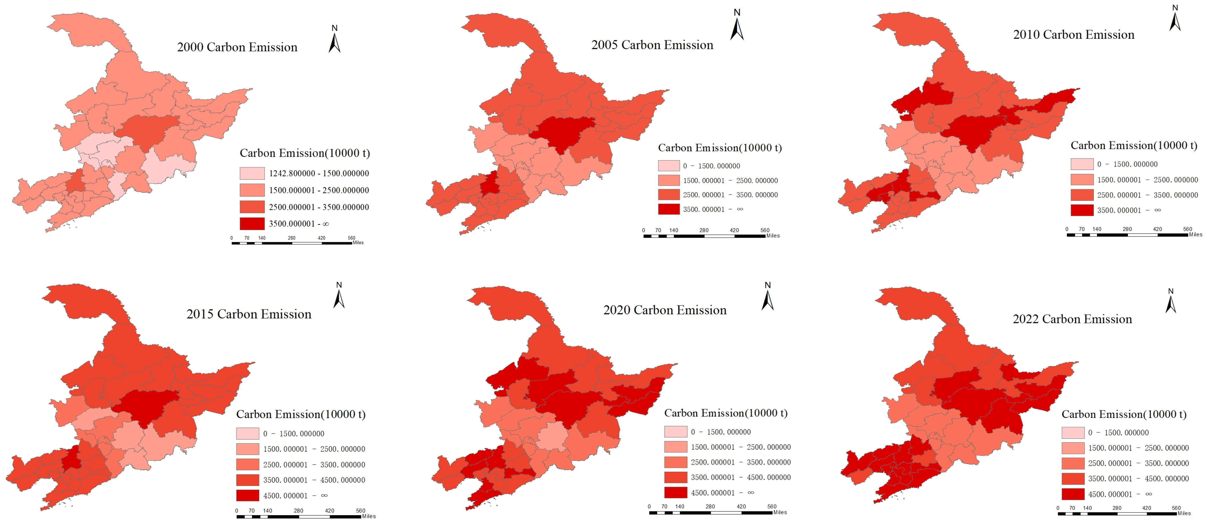
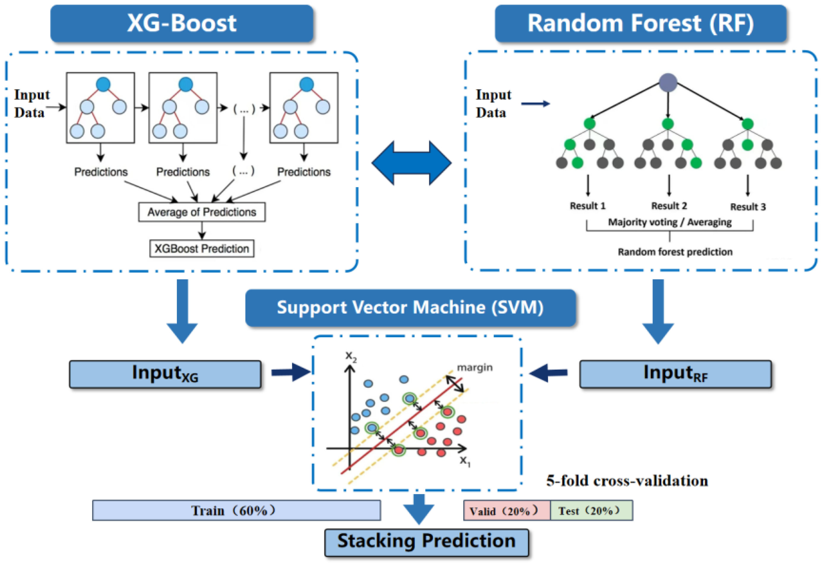

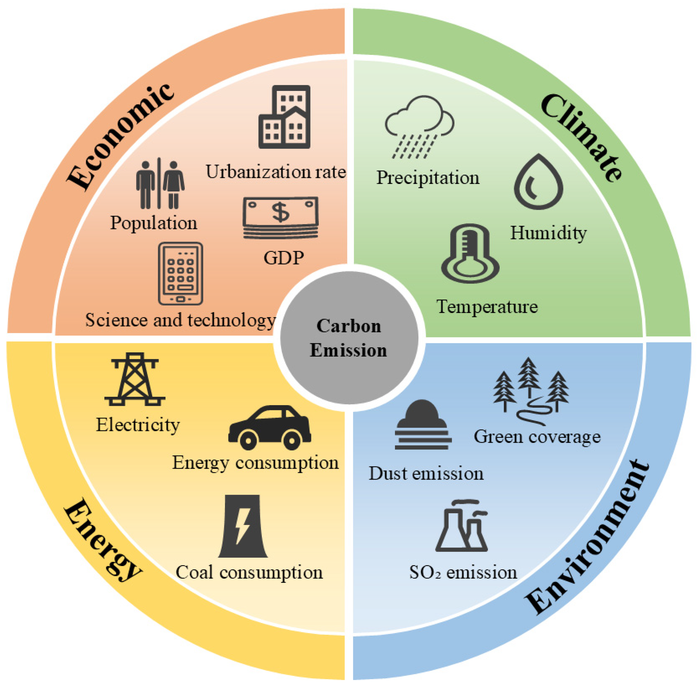
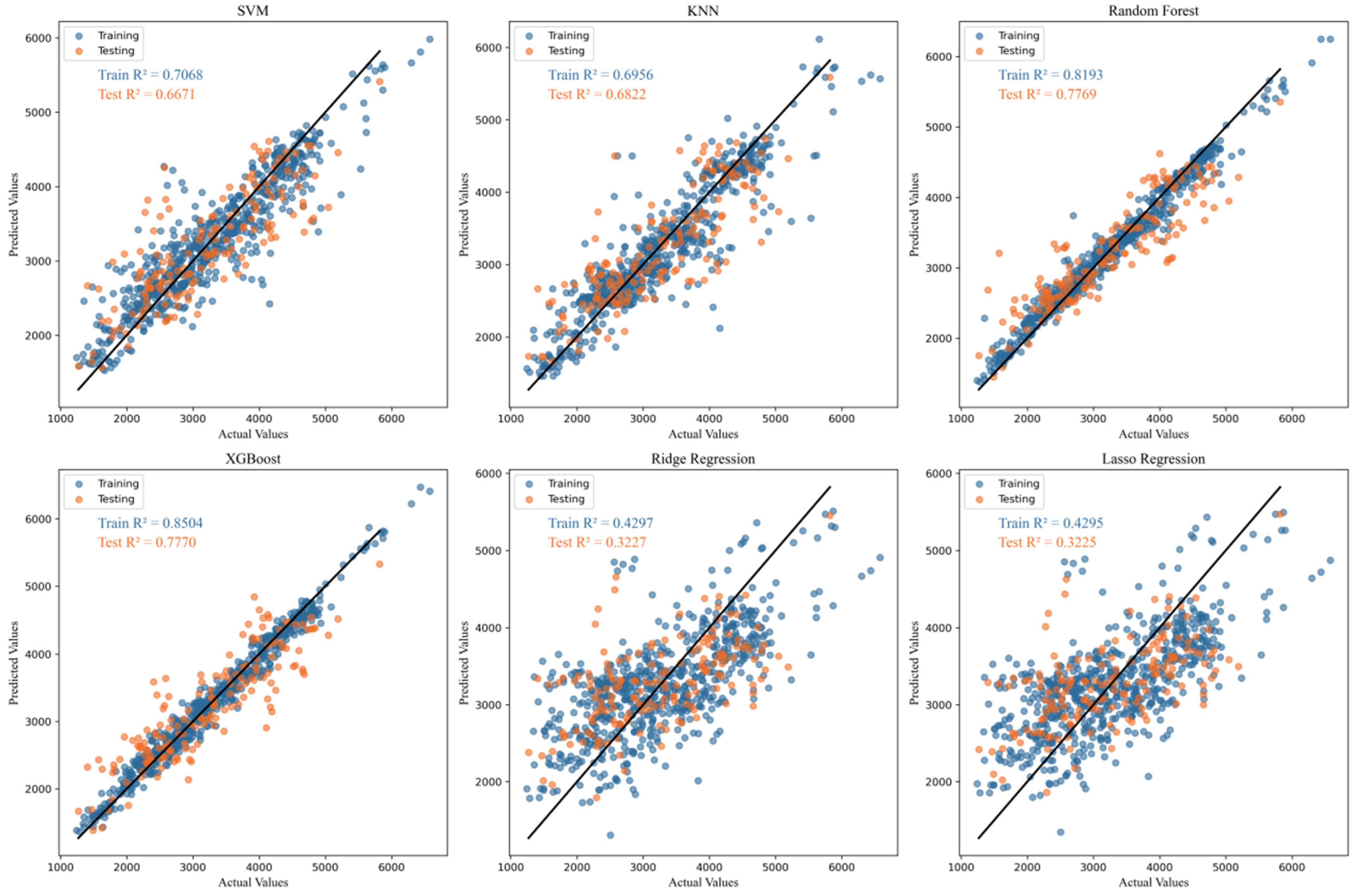
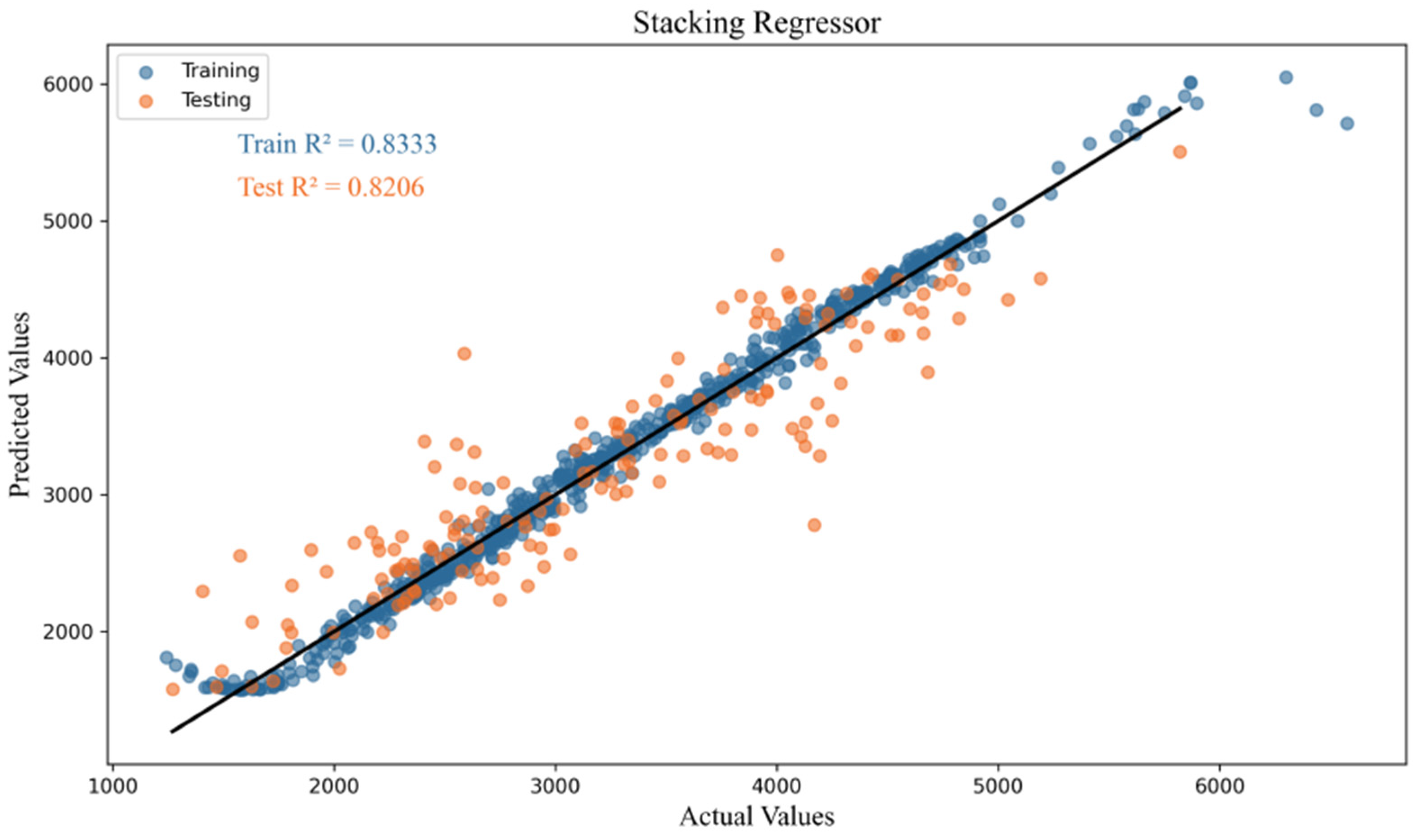
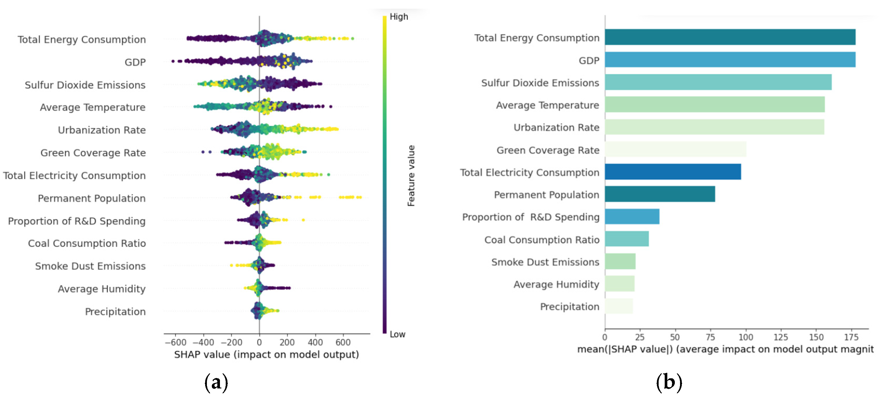
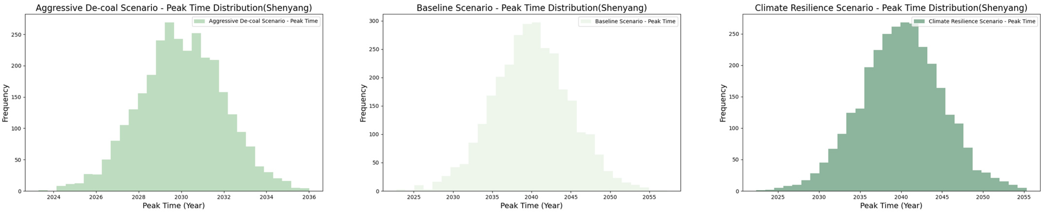
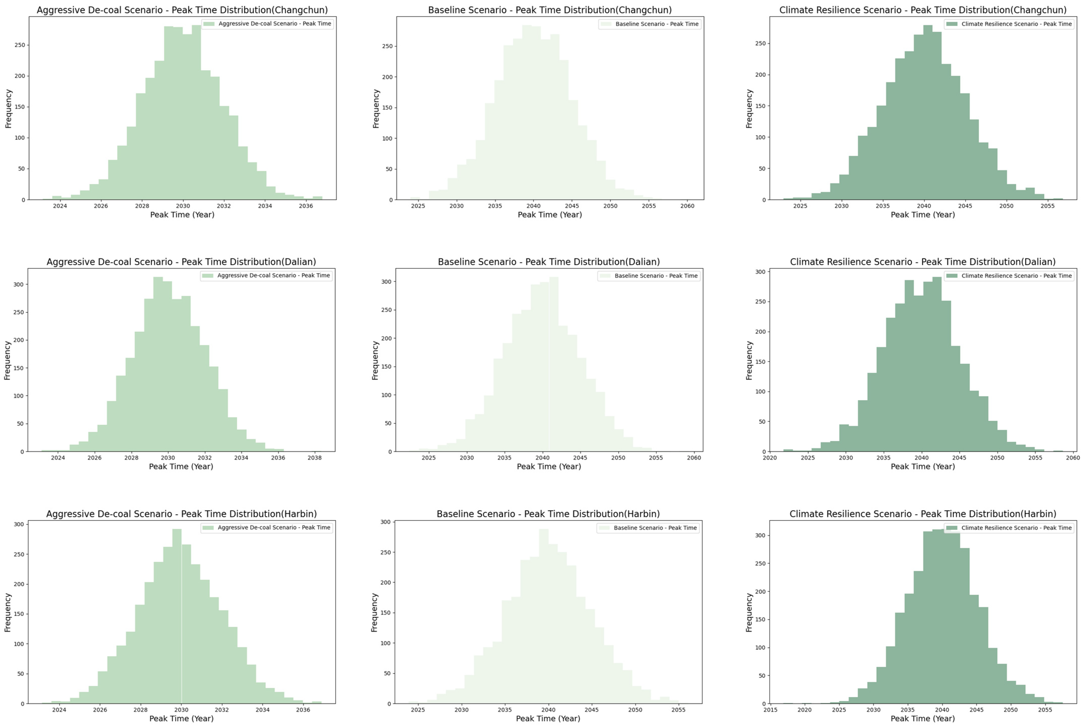
Disclaimer/Publisher’s Note: The statements, opinions and data contained in all publications are solely those of the individual author(s) and contributor(s) and not of MDPI and/or the editor(s). MDPI and/or the editor(s) disclaim responsibility for any injury to people or property resulting from any ideas, methods, instructions or products referred to in the content. |
© 2025 by the authors. Licensee MDPI, Basel, Switzerland. This article is an open access article distributed under the terms and conditions of the Creative Commons Attribution (CC BY) license (https://creativecommons.org/licenses/by/4.0/).