Evaluating the Spatial Relationships Between Tree Cover and Regional Temperature and Precipitation of the Yucatán Peninsula Applying Spatial Autoregressive Models

Abstract

Deforestation and forest degradation are important drivers of global warming, yet their implications on regional temperature and precipitation patterns are more elusive. In the Yucatán Peninsula, forest cover loss and deterioration has been rapidly advancing over the past decades. We applied local indicators of spatial association (LISA) cluster analysis and spatial autoregressive models (SAR) to evaluate the spatial relationships between tree cover and regional temperature and precipitation. We integrated NASA’s Global Forest Cover Change (GFCC) and WorldClim’s historical monthly weather datasets (2000–2015) to assess the effects of deforested, degraded, and dense forest land cover on temperature and precipitation distributions on the Yucatán Peninsula. LISA cluster analyses show warmer and drier conditions geographically coincide with deforested and degraded tree cover, but outliers allude to the potential influence of forest cover impacts on regional climate. Controlling spatial dependencies and including covariates, SAR models indicate that deforestation is associated with higher annual mean temperatures and minimum temperatures during dry and wet seasons, and decreased precipitation in the dry season. Degraded tree cover was related to higher maximum temperatures but did not relate to precipitation variability. We highlight the complex interactions between forest cover and climate and emphasize the importance of forest conservation for mitigating regional climate change.

1. Introduction

Deforestation and forest degradation in the tropics are significant drivers of global warming due to the associated emissions of greenhouse gases [1]. Carbon net flux from land use and land cover change is estimated to be 1.1 Pg C yr⁻¹ (2000–2010) [2,3] contributing up to 10% of the total global CO₂ emissions [4]. Since 1850, tropical forest cover has decreased by 30%, and most of the loss is of tropical moist deciduous (53%) and dry forest (70%) [5], having an important presence in Mesoamerica, yet intensely threatened by human pressure [6]. The impacts of forest degradation have been more difficult to assess and quantify since tree cover partly remains, nonetheless up to 69% of emissions from tropical forest landscapes can be attributed to degradation processes [7], defined as the gradual loss and capacity to provide ecosystem services and goods due to human induced disturbances, such as fire, logging, grazing, or fuel-wood collection [8]. Carbon emissions estimated from forest degradation in the tropics have amounted to 2.1 billion tons (0.4 Pg yr⁻¹) between 2005 and 2010 [9]. What is more, increased temperature and prolonged droughts brought by climate change can bring increased threats of fire and forest degradation that can add substantially to carbon emissions and further impact forest cover [5]. The negative impacts of forest loss and degradation on biodiversity and the livelihoods and resiliency of indigenous and rural communities across the tropics are also of concern [10,11,12], raising the importance of national and international efforts to conserve tropical forest cover.

The tropical forests of the Yucatán Peninsula, also known as the Selva Maya, extend across Mexico, Belize, and northern Guatemala and, after the Amazon, make up the largest relatively contiguous surface of tree cover, representing a vital region for climate change mitigation and biodiversity conservation [13,14]. Nevertheless, the Selva Maya is also heavily impacted by ongoing deforestation and degradation processes [15,16]. In the Mexican states of Campeche, Quintana Roo, and Yucatán, over 80,000 hectares of moist deciduous and dry tropical forest have been lost each year between 2001 and 2018 [15], making the region a deforestation hotspot [14]. Furthermore, gross deforestation has been higher after 2010, compared to the previous decade, and most of the forest conversion is for cattle (61%) and agricultural (38%) land uses [15]. The extent and impacts of forest degradation have been scarcely investigated in the region, in southern Quintana Roo, a study indicates that up to 50% of forest cover is degraded secondary forest [16], and other studies have revealed similar degradation patterns in the state of Yucatán [17]. Despite national commitments and international and local efforts to halt forest loss in the Yucatán Peninsula, deforestation and degradation trends remain unabated [15].

Compared to areas with forest cover, deforested areas globally, and especially in the tropics, exhibit higher temperatures, with increased diurnal and nocturnal warming [18]. The role of forest loss and degradation in global warming is well documented [19,20], and has led to initiatives such as REDD+ (Reduction in Deforestation and Degradation), promoted by the UNFCCC [21]. However, at regional and local scales, the effects of tree cover loss on climate variability remain less understood [22,23]. Forest loss affects local climate by altering energy and water cycles [24,25]. Tree cover contributes to climate regulation through evapotranspiration and albedo, with effects that vary by latitude [26]. While deforestation in higher latitudes may lead to cooling via increased albedo and snow reflection, in tropical regions it reduces evapotranspiration, enhancing warming despite albedo gains [24,27].

Reduced evapotranspiration can also result in decreased precipitation [27], and the removal of tree cover can alter the interception, infiltration, and runoff of rainfall, impacting the hydrological cycle [28]. Limited, tropical studies have shown that changes in forest cover are linked to variations in temperature and precipitation. A pantropical study found that losing 50% of the forest cover increased the land surface temperature (LST) by 1.1 °C, with gains in forest cover producing a similar cooling effect [26]. In Malaysia, LST was inversely related to forest NDVI [29]. Regarding precipitation, large-scale deforestation (e.g., in the Amazon) tends to reduce rainfall, whereas small-scale deforestation may increase it [25]. At local scales across the tropics, deforestation has been linked to warmer and drier conditions, particularly during the wet season, with rainfall reductions of 10–20% [25,30]. In both humid and dry tropical zones, forest loss can heighten the risk of droughts and floods [31], though other studies have reported mixed or inconclusive local precipitation responses [32,33].

Studies conducted through the monitoring of meteorological stations on the Yucatán Peninsula have observed significant changes in precipitation (a decrease of 12 mm) and temperature (an increase of 4 °C) since 1985 [34]. Additionally, in the Selva Maya, negative effects were found in the acquisition of organic phosphorus, an indicator of soil drought [35]. Furthermore, a perception analysis revealed that the population perceived an increase in temperature and a decrease in precipitation, primarily affecting those engaged in rainfed agriculture and fishing [36]. Thus, assessing the spatial relationships of forest cover loss and degradation with local and regional temperature and precipitation is vital to understanding climate change impacts on the Yucatán Peninsula. Although this research is lacking for the Selva Maya region, it is a necessary component for policy development and implementation to combat climate change, at national, state, and local levels, encouraging broad assessments of the effects of land cover change policies on regional and local climate phenomena, beyond global warming [31].

The increasing availability and application of earth observation data has been paramount in advancing spatial analyses to support research on global and regional environmental change [37]. Widely available forest datasets now include Global Forest Change [38], percent tree cover, canopy height, and cropland expansion, developed by the University of Maryland’s Global Land Analysis and Discovery (GLAD) lab [39]. NASA’s (National Aeronautics and Space Administration) Global Forest Cover Change (GFCC) products also contribute to remotely sensed data [40], along with forest biomass and carbon density datasets [41,42,43]. For humid tropical forests, the European Commission Joint Research Centre provides deforestation and degradation data from 1990 to 2019 [44], though it excludes dry tropical forests. Climate geoinformation datasets are also widely used; WorldClim offers historical, future, and bioclimatic variables [45], with similar data available from CHELSA (climatologies at high resolution for the earth’s land surface areas) [46] and ERA5 from the Copernicus Climate Change Service [47].

The Future Earth program, created by the International Science Council, promotes research on land use and land cover change, ecosystem services, and human-environment interactions across scales [48]. Numerous studies have combined forest cover, land use, and climate datasets to analyze global and regional changes. For example, these include forest loss and recovery effects on surface temperature at a global scale [26]; combined use of WorldClim and Amazonian forest change data to assess impacts on primate habitat suitability [49] and plant diversity [50]; and projected effects of deforestation and climate change on tree species distributions in Ecuador [51] and the Brazilian Amazon [52].

Spatial analyses and statistics are necessary tools to adequately explore the relationships between forest cover change and climate, natural resources or environmental services using geoinformation. The premise of spatial statistics is that earth observations exist in the context of a geographical space and may have local spatial characteristics [48]. Consequently, spatial data tend to exhibit spatial autocorrelation and usually clustered distributions due to the similarity between observations closest to each other, which can increase uncertainty and error when evaluating relationships with standard inferential statistics [53]. Spatial autocorrelation and spatial autoregression analyses allow for the identification of spatial patterns and the assessment of relationships between geographically represented variables. Spatial autoregressive models (SAR) are typically used to explore spatial relationships, since these models can address spatial autocorrelation problems [54,55,56].

In this study, we evaluated the spatial relationship of NASA’s GFCC tree cover data, categorized as persistent dense, deforested, and degraded tree cover, with long-term spatial distributions of the WorldClim historical monthly temperature and precipitation data (2000–2015) of Mexico’s Yucatán Peninsula. A geographical information system (GIS) was applied to analyze the geographical distributions and relationships between temperature and precipitation dependent variables with the independent variables of percent tree cover, and other spatial covariates. Moran’s I and local indicators of spatial association (LISA) were calculated to assess spatial autocorrelation and evaluate the distribution patterns of forest cover, temperature, and precipitation on the Yucatán Peninsula. We applied SAR models with fixed effects to determine the associations between tree cover (i.e., dense, deforested, and degraded) and temperature and precipitation conditions, annually and during the dry and wet seasons. Our SAR statistical model accounted for spatial autocorrelation of the dependent and independent variables of tree cover and other relevant geographical covariates representing regional environmental and socioeconomic conditions, thus improving the precision and predictive power of the models to evaluate deforestation and degradation associations with regional temperate and precipitation distributions [55].

2. Materials and Methods

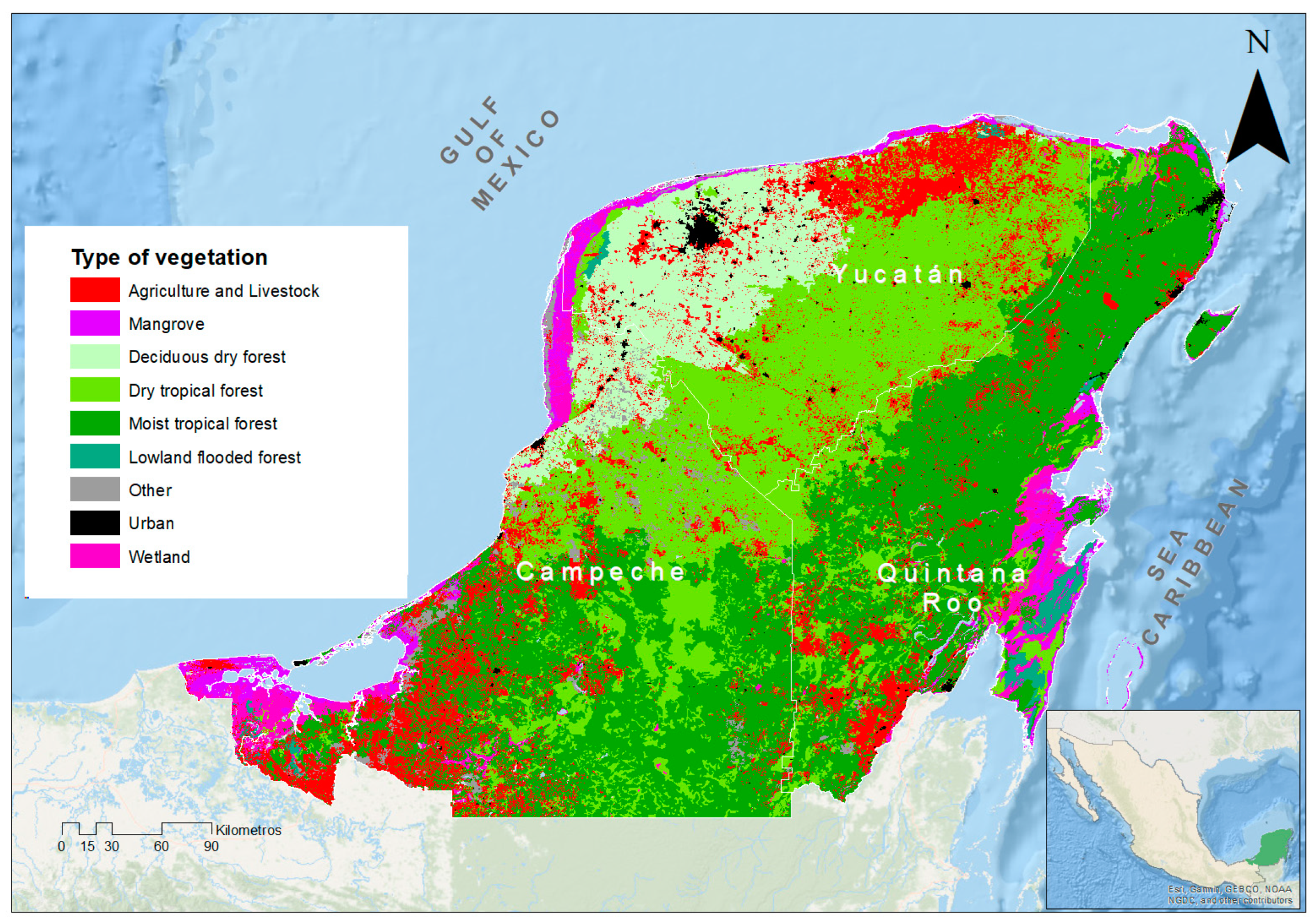
2.1. Study Area

The Yucatán Peninsula is in southeast Mexico and comprises the states of Campeche, Quintana Roo, and Yucatán with a total area of 147,243 km² [57]. Its western and northern coastlines are bordered by the Gulf of Mexico, the eastern coast by the Caribbean Sea, and its southern boundary is bordered by the countries of Belize and Guatemala. Due to its generally flat topography, karstic geology, and the terrain’s favorable infiltration capacity, there is little surface runoff and few streams, rivers, or waterways, with the exception of the Champotón River in the state of Campeche, and the Hondo River in the southeast of the state of Quintana Roo [58,59]. Even though the topography is mostly level, there are relief features and hilly terrain in the central and southern regions with a north to south elevation gradient that reaches altitudes up to 400 m, as well as a coastal to interior gradient [59,60]. The climate on the Yucatán Peninsula varies regionally. The main Köppen climate types consist of Aw, tropical wet and dry (Aw0, Aw1, and Aw2), and BS, semi-arid [61,62,63]. The eastern and southwestern regions of the peninsula are dominated by Aw1 climate, which has a pronounced dry season during the winter months, typically from November to April, and a rainy season from May to October, with peak rainfall occurring between June and September. Throughout the year, temperatures remain warm with minimal fluctuations. The average monthly temperature is 26 °C, with the summer months occasionally reaching maximum temperatures above 35 °C. The hottest period typically coincides with the end of the dry season. The northwestern region of the Yucatán Peninsula is characterized by Aw0 climate, with higher maximum temperatures averaging 36 °C [60], and a hotter climate compared to Aw1 in the east and south. The northwest and northern coastal regions have even hotter temperatures, in addition to semi-arid climate conditions (BS) [8].

The annual average precipitation on most of the peninsula varies from 1000 to 1200 mm. In the eastern coastal region and southwestern limits of the study area, the precipitation is greater (1500 to 2000 mm/year) with more evenly distributed rainfall. By contrast, the northwestern region of the Yucatán Peninsula has a drier climate (Aw0), with a highly pronounced dry season and relatively lower rainfall (500 to 800 mm/year). In the northernmost coastal region, rainfall is as low as 400 mm [61]. Extreme weather events are common on the peninsula. Tropical storms and hurricanes occur from June to November, affecting predominantly the eastern Caribbean coastline, often bringing flooding and affecting infrastructure, agriculture, and ecosystems [63,64,65]. Droughts primarily occur during the dry season in the northern and western regions leading to water scarcity and wildfires [66,67].

Leptosols are the predominant soil type distributed across half of the Yucatán Peninsula, characterized as shallow, rocky, fine to medium textured soils present in upland areas; Phaezoms and Luvisols cover close to 20% of the study area, and are characterized as darker, deeper soils, present on flat and rolling terrain, preferred for agricultural uses; Vertisols and Gleysols, also covering 20% of the study area, are characterized as grey, moist, clayey soils with poor drainage located in lowland areas and, in some cases, the flooded regions [58,68]. Natural vegetation is largely associated with precipitation and soil distributions on the Yucatán Peninsula (Figure 1) [69,70,71]. Tropical forest ecosystems are mostly represented by a medium-stature (15–25 m), moist, semi-evergreen forest distributed throughout the southern and eastern portions of the peninsula. The central and western regions contain dry tropical forest, characterized by medium-height, semi-deciduous forests with around 75% of trees shedding their leaves during the dry season. In the drier northwestern and northern regions, forests are deciduous and of low height (less than 10 m), with total leaf loss during the dry season. Moreover, semi-evergreen, low-stature flooded forests are present in the lowland depressions, where clayey soils with poor drainage are found, and mangrove forests, coastal dunes, and wetlands are present along the peninsular coastline [72,73,74].

The population distribution follows a center–periphery model of human settlements, with a high demographic concentration in major metropolitan areas such as Mérida, Cancún, Chetumal, and Campeche, and a pronounced population dispersion across approximately 30,000 rural settlements [68]. Economic activities of the Yucatán Peninsula are diverse. In Yucatán state, manufacturing, focused on textiles and food products, is a major economic component, but agriculture, centered on crops such as corn, soybean, and citrus fruits, provides an important source of income for rural communities [75]. Tourism also plays a significant role due to archaeological sites and beaches that attract both domestic and international visitors. Nevertheless, in Quintana Roo, with its Caribbean coast, tourism is the main economic activity, accounting for 86.5% of its gross domestic product (GDP), consisting of high-end resorts and hotels along the Riviera Maya that create jobs and local infrastructure [58]. Meanwhile, Campeche’s economy is primarily characterized by hydrocarbon extraction, which accounts for approximately 76.9% of its GDP, making it the state’s largest income generator, particularly through PEMEX’s (Mexican Petroleum) activities in the Gulf of Mexico. Agriculture and fishing play a lesser role but are very important to rural economies [58]. The state is a significant producer of cash crops, such as oil palm, soybean, sugarcane, and sorghum, in addition to cattle, for both national and international markets [75,76].

Cattle production, the expansion of commercial and mechanized agriculture, urban growth, and tourism development have led to pervasive deforestation and forest degradation processes in the Yucatán Peninsula [77,78]. The areas most affected by deforestation due to livestock farming include the southwest, center, and north of Campeche [79,80], the northeast of Yucatán [81], and the south of Quintana Roo [82]. Regarding mechanized agriculture, the most impacted areas are primarily located in the municipality of Hopelchén in Campeche, Tekax in Yucatán [83], and Bacalar in Quintana Roo [84,85]. The increase in mechanized production in Campeche and Quintana Roo has coincided with the growth of the Mennonite population [86]; while in Yucatán, it has been driven by agribusinesses [87]. In addition to the anthropogenic drivers of forest loss and degradation, forests in the region are also prone to frequent natural disturbances from hurricanes and fires [88], although they can be very resilient and quickly recover from natural and anthropogenic disturbances [89]. The tropical forest in the region, for the most part, is not pristine, but rather anthropogenic in nature [90,91], and in many rural communities, forest management for timber and traditional slash-and-burn practices (milpa) can aid in conserving forest cover and biodiversity in the study region landscape [92].

Figure 1. Land use and vegetation distribution in the study area (2018). (Source: [93]).

Figure 1. Land use and vegetation distribution in the study area (2018). (Source: [93]).

2.2. Spatial Data and Processing

We employ the percent tree cover data of the Global Forest Cover Change (GFCC) dataset from the Land Processes Distributed Active Archive Center (LPDAAC), distributed by the NASA Making Earth System Data Records for Use in Research Environments (MEaSUREs) Program [94]. Tree cover data, available for the years 2000, 2005, 2010, and 2015, are derived from the GFCC Surface Reflectance product of the Landsat 5 Thematic Mapper (TM) and the Landsat 7 Enhanced Thematic Mapper Plus (ETM+) images with 30 m resolution, combined with the Vegetation Continuous Fields (VCF) product from MODIS images with 250 m resolution [95]. The data consist of estimates of the percentage of land covered by woody vegetation taller than 5 m within 30 m pixels. Details regarding the methodology used to create the data are available in Sexton et al. [96]. The VCF scheme used to represent tree cover has been widely used to characterize forest vegetation types and gradients, as well as to monitor forest changes, such as deforestation and degradation [96].

The GFCC percent tree cover data [97] was downloaded with the geographical coverage of the Yucatán Peninsula, and for the 4 available years, totaling 64 images. The tree cover images were merged for each year and clipped to the extent of our study area, and empty pixel values were filled based on neighboring pixel values using the ISNULL and Focal Statistics functions in raster calculator. The percentage of tree cover was then reclassified to a range of values from 0 to 100%, since original GFCC values ranged from 0 to 87% for the Yucatán Peninsula. The percentage of tree cover was subsequently categorized as dense forest (>70% tree cover), degraded or secondary vegetation (30 to 70% tree cover), and deforested (<30% tree cover). This categorization was adopted to accurately capture deforested and forested areas in the study region, the latter defined by Hansen et al. [37] as having a canopy density of at least 30%, and, in addition, effectively to differentiate between secondary or degraded forests from mature forest ecosystems on the Yucatán Peninsula. The 70% tree cover threshold is used by FAO to define dense or closed mature forest cover [98,99]. Some areas that are categorized as degraded or secondary, specifically from human disturbances, may coincide with natural vegetation, such as savannas with trees or dwarf mangrove wetlands; however, these vegetation types are ultimately excluded in this study. Processing of spatial data was conducted with ArcGIS 10.8.

Regional temperature and precipitation data for the Yucatán Peninsula were obtained from the WorldClim Historical Monthly Weather Data developed by the Climatic Research Unit (CRU) of the University of East Anglia [100] and are available in the WorldClim 2.1 dataset [100]. We downloaded monthly weather data for the years 2000 to 2015, consisting of mean minimum and maximum temperature and mean precipitation with spatial resolution of 2.5 min, downscaled to 1 km² pixels [101]. The average for the years 2000 to 2015 for each temperature and precipitation parameter were calculated. Mean annual temperature, not available in the WorldClim Historical Monthly Weather Data, were obtained by calculating the monthly averages of minimum and maximum temperature for each year from 2000 to 2015. All raster calculations were performed with the Raster Calculator in ArcGIS 10.8.

Geographical factors that are most likely related to the spatial distribution and variability of temperature and precipitation parameters in the study area were included as covariates in our analysis. The spatial covariates used included elevation (15 m resolution), distance to urban areas, distance to roads, distance to water bodies [102], vegetation biomass for the year 2004 (30 m resolution) [103], land use and land cover in vector format [104], and temperature and precipitation climate regions on the Yucatán Peninsula based on the Köppen climate classification system, also in vector format [93]. The vector spatial data of land use and land cover and the Köppen climate regions were converted to raster data for our analyses, and distance values from spatial features (e.g., roads and urban centers) were calculated with the Euclidean Distance function and represented in raster format. ArcGIS 10.8 was applied for raster conversions and distance calculations. Since our goal was to assess the impact of tree cover on temperature and precipitation, controlling for baseline climatic variation (independent of forest cover) was crucial. Indeed, the SAR model covariates included are intended to isolate the effect of tree cover categories from other natural and geographical variability that can also influence climate temperature and precipitation distributions. Covariates of land use and distance to roads and urban areas are used to include human presence and influence factors in the analyses.

Table 1. Description of spatial variables used in this study.

Variables	Symbol	Type of Variable	Description	Scale of Measurement
Temperature	TMP	Dependent	Mean annual temperature (2000–2015)	Continuous
Minimum Temperature	MINT	Dependent	Mean minimum annual temperature (2000–2015)	Continuous
Maximum Temperature	MAXT	Dependent	Mean maximum annual temperature (2000–2015)	Continuous
Dry Season Temperature	DTEMP	Dependent	Mean temperature during the dry season (December–May 2000–2015)	Continuous
Minimum Dry Season Temperature	DMINT	Dependent	Mean minimum temperature during the dry season (December–May 2000–2015)	Continuous
Maximum Dry Season Temperature	DMAXT	Dependent	Mean maximum temperature during the dry season (December–May 2000–2015)	Continuous
Wet Season Temperature	WTEMP	Dependent	Mean temperature during the wet season (June–November 2000–2015)	Continuous
Minimum Wet Season Temperature	WMINT	Dependent	Mean minimum temperature during the wet season (June–November 2000–2015)	Continuous
Maximum Wet Season Temperature	WMAXT	Dependent	Mean maximum temperature during the wet season (June–November 2000–2015)	Continuous
Annual Precipitation	PPT	Dependent	Mean annual precipitation (2000–2015)	Continuous
Dry Season Precipitation	DPPT	Dependent	Mean annual precipitation during the dry season (December–May 2000–2015)	Continuous
Wet Season Precipitation	WPPT	Dependent	Mean annual precipitation during the wet season (June–November 2000–2015)	Continuous
Forest Cover 2000–2015	FOR	Fixed	Percent tree cover greater than 70% during years 2000, 2005, 2010, and 2015	Categorical
Degradation 2000–2015	DEGR	Fixed	Percent tree cover from 30% to 70% during years 2000, 2005, 2010, and 2015	Categorical
Deforestation 2000–2015	DEFOR	Fixed	Percent tree cover below 30% during years 2000, 2005, 2010, and 2015	Categorical
Biomass	BIO	Covariate	Above ground biomass (kg ha−1) with 30 m resolution	Continuous value
Elevation	ELEV	Covariate	Elevation above sea level in meters with 15 m resolution	Continuous value
Urban Centers	URB	Covariate	Distance to main urban areas in meters	Continuous value
Water Bodies	WAT	Covariate	Distance to water bodies in meters	Continuous value
Roads	RDS	Covariate	Distance to roads in meters	Continuous value
Vegetation Type	VEG	Covariate	Vegetation type or ecosystem and land use	Integer value
Minimum Temperature Zones	ZMINT	Covariate	INEGI minimum temperature zones	Integer value
Maximum Temperature Zones	ZMAXT	Covariate	INEGI maximum temperature zones	Integer value
Precipitation Zones	ZPPT	Covariate	INEGI precipitation regions	Integer value

summarizes the spatial variables employed in this study.

2.3. Sampling Design

We extracted and developed a point dataset containing values for each of the spatial variables (Table 1) to evaluate spatial autocorrelation and to build spatial autoregressive models that tested the relationships between temperature and precipitation and tree cover. A vector layer (shapefile) of 1 km² quadrants was generated across the entire Yucatán Peninsula totaling 149,849 km². Within each quadrant, the average of all dependent and independent spatial variables were calculated using the Tabulate Areas function in Spatial Analyst of ArcGIS 10.8. Subsequently, a set of 118,218 quadrants were selected from the total quadrants, which excluded those that had changed their forest cover category (i.e., dense forest, degraded forest, and deforested) from 2000 to 2015 and those that contained water bodies and non-forest vegetation types, such as wetlands, typically located along coastal areas and not subject to human disturbance. This way, we avoided sampling unsuitable quadrants for our statistical analyses and ensured that the forest cover category had been consistent during the 15-year range of data used, avoiding spatial and temporal non-stationarity, and ensuring permanent forest cover categories. Finally, 3000 points were generated within the center of randomly selected quadrants stratified according to tree cover category: 1000 points in deforested quadrants, 1000 points in degraded forest quadrants, and 1000 points in dense forest quadrants.

2.4. Statistical Analysis

Global Moran’s I was calculated to assess spatial autocorrelation of the climate and forest cover variables represented by the random point dataset. Spatial autocorrelation measures how geographical phenomena are grouped in general. The Moran’s I indicator is a weighted correlation coefficient used to detect deviations from spatial randomness, determining if neighboring areas are more similar than expected under the null hypothesis. The values of Moran’s I range from −1 (perfect dispersion) to 1 (perfect correlation), and values close to zero indicate random patterns. For statistical hypothesis testing, the value of Moran’s I is transformed into a Z-score, where values greater than 1.96 and less than −1.96 indicate statistically significant spatial autocorrelation at the 5% level [54].

LISA (local indicator of spatial association) cluster analysis was applied to explore spatial autocorrelation and distribution patterns [105,106]. LISA cluster analysis separates the Global Moran’s I indicator into sub-indicators for each spatial unit enabling the detection of local spatial clusters and types of associations [107]. The scatter plot and spatial distribution of local Moran’s I generated by LISA is used to assess spatial autocorrelation, identifying data points and geographical regions where high–high, low–low values are clustering, or where dissimilar values (low–high and high–low) which could represent locations with low values surrounded by neighbors with high values, and vice versa [54]. This analysis provides a useful tool to visualize spatial associations. LISA analyses were conducted for the forest cover category and climate variables using the Cluster and Outlier Analysis (Anselin Local Moran′s I) tool in ArcGIS 10.8 [108]. Moreover, inverse distance weighting (IDW) raster surface interpolation maps were produced for forest cover and climate variables to assist in the visualization of data spatial distribution using the IDW tool in ArcGIS 10.8.

Forest cover and climate variables tend to have clustered distributions in the landscape warranting the application of spatial autoregressive (SAR) models to assess the relationship between them. We used STATA 17.0 to construct SAR models that account for the spatial autocorrelation of clustered data by integrating spatial weighting matrices that parametrize the spatial relationship between the data points using inverse distance weighting. These matrices are added to a linear regression model (OLS) as a term to represent spatial lag, the effect of an outcome in one location on the outcome of a neighboring location and spatial error, the errors of neighboring points [109]. For the SAR models of this study, percent forest cover was applied as a fixed effect variable (Table 1), with the categories of dense forest, deforested, and degraded forest assumed to be measured without error. The general form of the SAR model with fixed effects can be expressed as follows:

Y = λ W Y + Xβ + μ + ε

(1)

where

-

Y is the dependent variable vector (e.g., mean annual temperature).

-

λ is the spatial autoregressive coefficient capturing the degree of spatial dependence in Y.

-

W is the spatial weights matrix defining the relationships between spatial units.

-

X is the matrix of independent variables.

-

β is the coefficient vector for X.

-

μ is the fixed effects capturing unobserved heterogeneity (i.e., forest cover category effects).

-

ε is the error term.

Fixed effects account for unobservable characteristics that are constant within groups, or over time, but vary across them. The spatial weights matrix, W, is a key element, often based on geographical proximity or network connections. The pseudo R² in geospatial analyses measures the proportion of variability in the dependent variable explained by the model, considering the spatial structure of the data. Although interpreted similarly to R² in traditional regression models, the pseudo R² accounts for spatial dependency. Unlike the R² of traditional OLS regression, the pseudo R² in SAR models is not a direct measure of explained variance, but rather a relative indicator of model fit that accounts for spatial dependencies. In spatial econometric research, pseudo R² values are commonly interpreted to be moderate when between 0.4 and 0.6 and strong when between 0.6 and 0.8 and are most useful for comparing competing spatial models rather than establishing absolute thresholds. SAR models have been applied in a diversity of studies, including modelling air pollution [110], assessing relationships between obesity and socioeconomic factors [111], vulnerability factors to natural disasters [112], and water use analysis [113].

3. Results

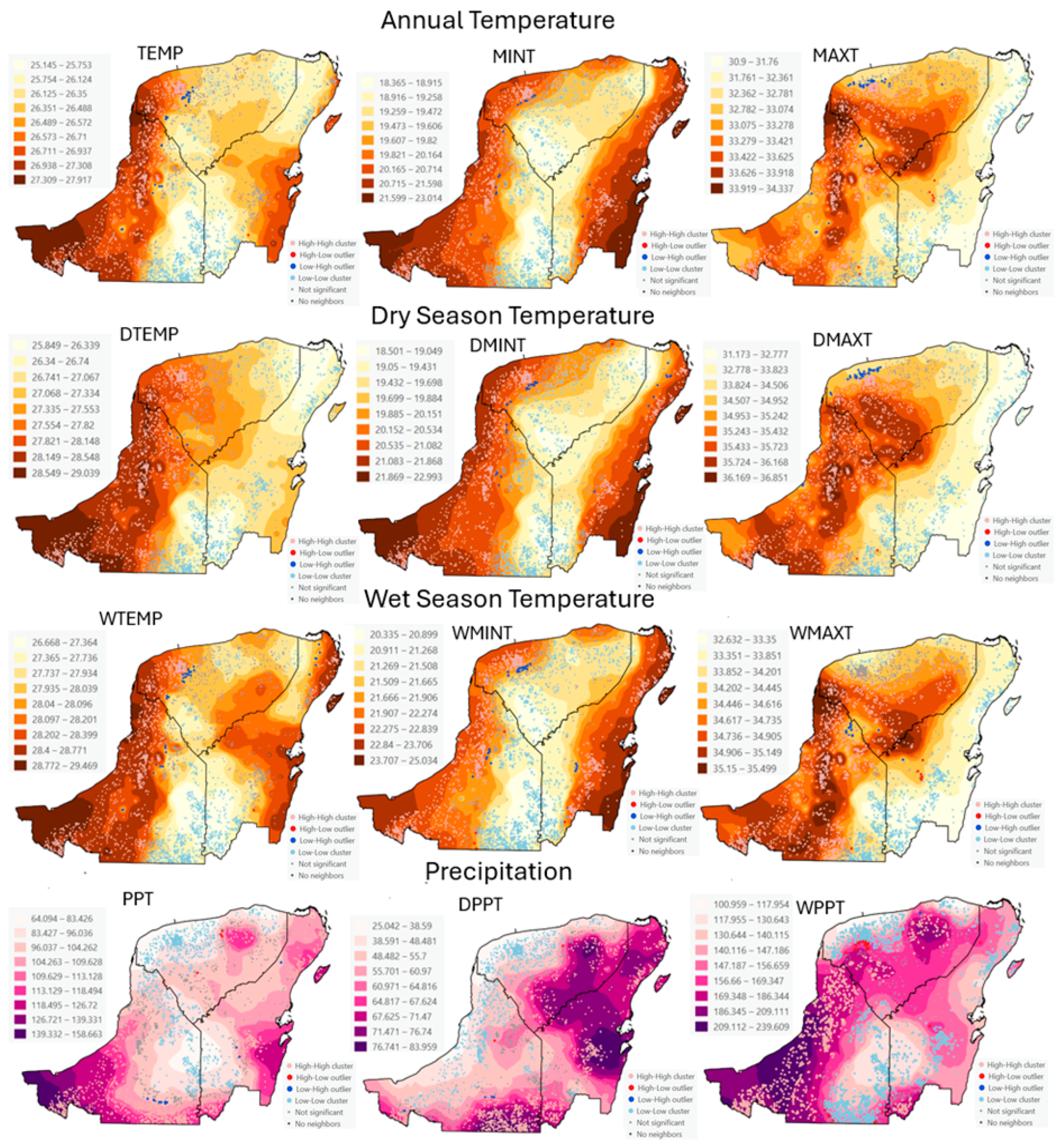
3.1. Spatial Distribution of Forest Cover and Climate

A geographical portrayal of spatial autocorrelation allows for the assessment of distributions of georeferenced forest cover and climate data on the Yucatán Peninsula, and in particular how neighboring spatial units are associated. The LISA analysis produces indicators of spatial association (Local Moran′s I), identifying clusters of autocorrelated or dissimilar data values, thus also identifying spatial outliers and providing a localized and geographical perspective on how spatial data behaves in specific areas. A high positive Local Moran′s I indicates that a value point is part of a cluster, and a high negative indicator shows that the value is a spatial outlier. When applied to spatial temperature and precipitation data, LISA can help reveal patterns and anomalies that might relate to forest cover.

Figure 2 shows the LISA and IDW results for forest cover (deforested, degraded, and dense tree cover) distribution on the Yucatán Peninsula. Global Moran′s I index was high (0.77), showing a significant clustered spatial autocorrelation (z = 189.12, p > 0.001), as expected. Clusters of high–high (pink) values (deforested) made up 59% of the data values, mostly representing long-term forest loss regions that coincide with cattle production and commercial agricultural land uses. These deforested clusters were notable in the northern and western regions, in the states of Campeche and Yucatán, respectively, as well as in major urban centers such as Merida, Cancún, and Campeche. Clusters of low–low values (light blue) consisted of 32% of the spatial units and were concentrated in forest areas distributed in the southern and eastern portion of the peninsula, in the states of Campeche and Quintana Roo, that overlap mostly with tropical moist forest vegetation rather than dry forests. Moreover, high–low outliers (red) represented deforestation and degradation fronts, and were located along the eastern and western limits of the Calakmul Biosphere Reserve in southeast Campeche, the southern and central portions of Quintana Roo, and eastern Yucatán, while low–high values (blue) indicated where larger forest remnants remain within long-term deforested areas in the state of Campeche and Yucatán.

Figure 3 shows the combined LISA and IDW results for temperature and precipitation variables. Not surprisingly, Global Moran’s I for all temperature and precipitation dependent variables demonstrated an even higher clustered spatial autocorrelation compared to tree cover data (Global Moran’s I > 0.90; z > 220; p > 0.001), which strongly justified applying SAR models to test relationships between tree cover. High–high annual TMP values (pink) were clustered in the western region of the Yucatán Peninsula and made up 37% of the sample points, while low–low values (light blue) were clustered in the central and eastern portions and contained 37% of the values. Another 25% of the data values were non-significant showing no statistically significant autocorrelation. These non-significant points contributed to reducing spatial dependence and strengthening the SAR models to test relationships with tree cover. These non-autocorrelated data points were scattered in the central and eastern portion of the Yucatán Peninsula. There were few outliers, only 28 reporting low temperatures among high temperature neighbors (blue), highlighting local anomalies, and were present in the central and northwest regions of the peninsula.

High–high (pink) minimum temperatures (MINT) were clustered in the western portion of the study area, but also appeared in the eastern coastal region, representing 42% of spatial units, while low–low (light blue) or cooler minimum temperatures were clustered in the central region and represented 46% of data points. Non-significant points (10%) are located between western high–high and central low–low clusters.

MAXT LISA results indicated a shift of maximum temperatures towards the central region of the Yucatán Peninsula, where high–high clustered values predominated (50%) and occupied most of the western and northern states of Campeche and Yucatán respectively. Low–low values (34%) with cooler maximum temperatures were clustered in southeast Campeche and the state of Quintana Roo. Low–high (blue) outliers were in the northwest, and few high–low outliers (red) were scattered in south and central Quintana Roo. Non-significant spatial units comprised 14% of the data values and were in the northern portion of the peninsula and central and southern Campeche. Dry and wet season mean, minimum, and maximum temperatures, as displayed in Figure 3, showed similar clustering of high–high and low–low values, and proportions and distributions of outliers and non-significant values as the yearly temperature values described above.

LISA results for annual precipitation (Figure 3) showed high–high values located in southwest, south, and eastern regions of the Yucatán Peninsula, and comprised 41% of the data points. Low–low values were clustered in the central and northwestern regions, and made up 37.5% of the values. Non-significantly autocorrelated data made up 22% of the data points, and were distributed between high–high and low–low clusters, only a few outliers were found. During the dry season, higher precipitation values moved eastward, with high–high values (41%) clustered in southern Campeche, eastern Quintana Roo, and southeast Yucatán. Low–low values were distributed in the western and northern portions of the peninsula, and comprised 38.5% of data values. Non-significant local values (18.5%) were distributed in the central region. During the wet season, high–high precipitation clusters were mostly distributed in the southwest and northeast of the Yucatán Peninsula, and made up 31% of the data points. Low–low values comprised 52% of the data points, and clusters were present in the south and northeastern region, and in the northern coastal region of Yucatán state. Non-significant values made up 16% of the Yucatán Peninsula, and were distributed across the study area.

3.2. Spatial Relationship Between Forest Cover and Climate

The distribution of deforested and degraded tree cover on the Yucatán Peninsula, mostly present in the states of Campeche and Yucatán, also corresponded to regions where temperatures were higher. Moreover, the western and northern regions of the peninsula were also characterized by a drier climate. The SAR models captured the regional clustering and spatial dependencies of the dependent climate variables, and the inclusion of the fixed effects variable of tree cover (dense forest, deforested, degraded) allowed the models to control confounding variables, accounting for unobserved heterogeneity.

Table 2. Results of spatial autoregressive model for mean annual temperature (TEMP), mean annual minimum temperature (MINT), and mean annual maximum temperature (MAXT) from 2000 to 2015.

Variables	TEMP	MINT	MAXT
	Coefficient (SE)	Coefficient (SE)	Coefficient (SE)
DEGR	0.007 (0.015)	0.040 (0.027)	0.044 (−0.023)
DEFOR	0.062 ** (0.020)	0.123 *** (0.035)	0.044 (−0.030)
BIO	1.21 × 10−3 * (6.13 × 10−4)	2.78 ** (1.10 × 10−3)	−4.50 × 10−3 *** (−9.31 × 10−4)
ELEV	−3.25 × 10−3 *** (8.35 × 10−5)	−5.31 × 10−3 *** (1.423 × 10−4)	−1.06 × 10−3 *** (1.26 × 10−4)
URB	0.0000014 (7.51 × 10−7)	0.0000165 *** (1.37 × 10−6)	−3.73 × 10−6 *** (1.15 × 10−6)
WAT	−5.17 × 10−6 *** (5.29 × 10−7)	−0.000012 *** (1.00 × 10−6)	1.41 × 10−6 (8.07 × 10−7)
RDS	−1.21 × 10−6 (1.35 × 10−6)	7.86 × 10−6 ** (2.53 × 10−6)	−7.87 × 10−6 *** (2.07 × 10−6)
VEG	−1.1429 × 10−3 (1.79 × 10−3)	−0.0139 *** (3.13 × 10−3)	0.015 *** (2.71 × 10−3)
ZMINT	0.051 *** (3.46 × 10−3)	0.151 *** (6.37 × 10−3)	−0.053 *** (5.27 × 10−3)
ZMAXT	0.034 *** (3.89 × 10−3)	−0.061 *** (7.02 × 10−3)	0.161 *** (5.94 × 10−3)
ZPPT	1.37 × 10−4 *** (2.7 × 10−5)	5.38 × 10−4 *** (4.45 × 10−5)	−8.65 × 10−5 * (4.12 × 10−5)
Constant	24.601 *** (0.145)	19.719 *** (0.259)	28.052 *** (0.222)
Spatial Lag	−1.41 × 10−3 (1.21 × 10−3)	−0.011 *** (2.30 × 10−3)	0.010 *** (1.46 × 10−3)
Spatial Error	2.674 *** (0.034)	3.542 *** (0.073)	2.639 *** (0.032)
Model Parameters	n = 3000 Wald Chi2 (12) = 4710.16 Prob > Chi2 = 0.000 Pseudo R2 = 0.541	n = 3000 Wald Chi2 (12) = 6989.23 Prob > Chi2 = 0.000 Pseudo R2 = 0.677	n = 3000 Wald Chi2 (12) = 3188.45 Prob > Chi2 = 0.000 Pseudo R2 = 0.546

* p < 0.05, ** p < 0.01, *** p < 0.001.

shows the SAR model results for TEMP, MINT, and MAXT dependent variables.

A significant positive association between lack of tree cover and mean annual temperature (β = 0.062, p < 0.01) suggested that areas subjected to long-term deforestation (DEFOR) exhibited higher annual mean temperatures (TMP), compared to forested regions. However, degraded tree cover (DEGR) did not show a significant relationship with annual temperature (β = 0.007, p > 0.05). Biomass (BIO) was positively associated with mean temperature (β = 0.001, p < 0.05), but weakly significant. However, elevation (ELEV) exhibited a significant negative relationship (β = −0.0032, p < 0.001), consistent with cooler temperatures at higher altitudes. Proximity to water bodies (WAT) was also associated with lower mean annual temperature (β = −5.17 × 10⁻⁶, p < 0.001). The spatial error term is highly significant (β = 2.674, p < 0.001), reflecting residual spatial autocorrelation, while the spatial lag term is insignificant (β = −0.0014, p > 0.05), reflecting less spatial dependence in the dependent variable. The model demonstrates moderate explanatory power (pseudo-R² = 0.54).

Permanently deforested areas (DEFOR) had a significant relationship with higher minimum temperature (MINT) (β = 0.123, p < 0.001), highlighting its impact on nighttime thermal conditions. Degraded tree cover (DEGR), however, was not significantly related to minimum temperature (β = 0.040, p > 0.05). Biomass (BIO) was positively associated with minimum temperature (β = 0.0028, p < 0.01), suggesting its possible role in mitigating nocturnal cooling. Elevation (ELEV) had a strong negative relationship (β = −0.0053, p < 0.001), reinforcing the inverse relationship between altitude and temperature. Urban proximity (URB) was significantly related to higher minimum temperature (β = 0.000016, p < 0.001), reflecting potential urban heat island effects. Conversely, distance to water bodies (WAT) was significantly associated with lower minimum temperature (β = −0.000012, p < 0.001). Spatial lag (β = −0.0113, p < 0.001) and spatial error (β = 3.542, p < 0.001) effects were significant, indicating substantial spatial dependencies in minimum temperatures. The model showed strong explanatory power (pseudo-R² = 0.68).

Maximum temperatures (MAXT) were not significantly related to either deforested (DEFOR) or degraded (DEGR) tree cover (β = 0.044, p > 0.05). Biomass (BIO) exhibited a significant negative relationship with maximum temperature (β = −0.0045, p < 0.001), emphasizing its capacity to moderate extreme heat. Elevation (ELEV) again shows a negative association with maximum temperature (β = −0.0011, p < 0.001); unexpectedly, urban proximity (URB) had a negative relationship with maximum temperature (β = −3.73 × 10⁻⁶, p < 0.001). Spatial lag (β = 0.0101, p < 0.001) and spatial error (β = 2.639, p < 0.001) terms were significant, pointing to strong spatial dependencies in maximum temperature patterns. The model’s explanatory power was moderate (pseudo-R² = 0.55).

Table 3. Results of spatial autoregressive model for mean temperature (DTEMP), mean minimum temperature (DMINT), and mean maximum temperature (DMAXT) during the dry season from 2000 to 2015.

Variables	DTEMP	DMINT	DMAXT
	Coefficient (SE)	Coefficient (SE)	Coefficient (SE)
DEGR	0.114 *** (0.021)	0.060 (0.033)	0.229 *** (0.034)
DEFOR	0.178 *** (0.027)	0.167 *** (0.042)	0.238 *** (0.044)
BIO	7.22 × 10−4 (8.42 × 10−4)	4.52 × 10−3 *** (1.31 × 10−3)	−5.54 × 10−3 *** (1.36 × 10−3)
ELEV	−2.58 × 10−3 *** (1.13 × 10−4)	−5.36 × 10−3 *** (1.72 × 10−4)	1.76 × 10−4 (1.85 × 10−4)
URB	−1.42 × 10−6 (1.04 × 10−6)	1.51 × 10−5 *** (1.64 × 10−6)	−1.04 × 10−5 *** (1.66 × 10−6)
WAT	−3.44 × 10−6 *** (7.31 × 10−7)	−0.0000135 *** (1.18 × 10−6)	6.72 × 10−6 *** (1.17 × 10−6)
RDS	−5.69 × 10−6 ** (1.87 × 10−6)	5.06 × 10−6 (2.99 × 10−6)	−1.34 × 10−5 *** (3.00 × 10−6)
VEG	−6.59 × 10−4 (2.44 × 10−3)	−0.019 *** (3.76 × 10−3)	0.019 *** (3.96 × 10−3)
ZMINT	0.038 *** (4.77 × 10−3)	0.164 *** (7.60 × 10−3)	−0.092 *** (7.66 × 10−3)
ZMAXT	0.108 *** (5.37 × 10−3)	−0.036 *** (8.47 × 10−3)	−1.26 × 10−4 * (5.98 × 10−5)
ZPPT	1.199 × 10−4 *** (3.74 × 10−5)	5.06 × 10−4 *** (5.63 × 10−5)	1.199 × 10−4 ** (3.74 × 10−5)
Constant	22.899 *** (0.201)	18.761 *** (0.315)	25.768 *** (0.322)
Spatial Lag	0.013 *** (1.57 × 10−3)	5.14 × 10−3 (2.90 × 10−3)	0.021 *** (2.04 × 10−3)
Spatial Error	2.621 *** (0.019)	3.065 *** (0.047)	2.509 *** (0.040)
Model Parameters	n = 3000 Wald Chi2 (12) = 4173.27 Prob > Chi2 = 0.000 Pseudo R2 = 0.484	n = 3000 Wald Chi2 (12) = 4316.73 Prob > Chi2 = 0.000 Pseudo R2 = 0.559	n = 3000 Wald Chi2 (12) = 3968.32 Prob > Chi2 = 0.000 Pseudo R2 = 0.603

* p < 0.05, ** p < 0.01, *** p < 0.001.

shows the SAR model results for temperature dependent variables during the dry season (DTEMP, DMINT, and DMAXT). Deforested tree cover (DEFOR) was significantly associated with higher temperature during the dry season (DTEMP) (β = 0.178, p < 0.001). Degraded tree cover (DEGR) was also significantly related to higher mean dry season temperature (β = 0.114, p < 0.001), although its effect was less pronounced compared to deforestation. Biomass (BIO) had no significant relationship (β = 0.0007, p > 0.05), while elevation (ELEV) was negatively related to temperature during the dry season (β = −0.0026, p < 0.001). Proximity to water bodies (WAT) was associated with lower dry season temperature (β = −3.44 × 10⁻⁶, p < 0.001), while distance to roads (RDS) was negatively related to dry season temperature (β = −5.69 × 10⁻⁶, p < 0.01). Spatial effects were significant, both spatial lag (β = 0.0127, p < 0.001) and spatial error (β = 2.621, p < 0.001), and reflected spatial dependencies. The model had moderate explanatory power (pseudo-R² = 0.48).

Deforested areas (DEFOR) also had a strong and significant association with warmer minimum temperature during the dry season (DMINT) (β = 0.167, p < 0.001), but degraded tree cover (DEGR) was not significantly related to minimum temperature during the dry season (β = 0.060, p > 0.05). Biomass (BIO) was positively associated with minimum temperature (β = 0.0045, p < 0.001), suggesting its role in mitigating nocturnal cooling during the dry season. Elevation (ELEV) had a negative cooling association (β = −0.0054, p < 0.001); proximity to water bodies (WAT) also showed a negative relationship with minimum temperature (β = −0.000013, p < 0.001), while urban proximity (URB) was related to higher minimum temperatures during the dry season (β = 0.000015, p < 0.001). Spatial dependencies were evident in the significant spatial error term (β = 3.065, p < 0.001), while spatial lag was not significant (β = 0.005, p > 0.05). The model exhibited moderate explanatory power (pseudo-R² = 0.56), comparable to the annual model for minimum temperature (MINT).

Areas devoid of tree cover (DEFOR) also had a significant association with higher maximum temperature during the dry season (DMAXT) (β = 0.238, p < 0.001), as did areas with degraded tree cover (DEGR) (β = 0.229, p < 0.001). Biomass (BIO) showed a negative association or cooling relationship (β = −0.0055, p < 0.001), likely due to its role in reducing heat extremes. Elevation (ELEV) was not significantly related to maximum temperature (β = 0.00018, p > 0.05), while proximity to roads (RDS) (β = −0.000013, p < 0.001) and water bodies (WAT) (β = 0.000007, p < 0.001) demonstrated unexpected opposing effects on maximum temperature during the dry season. The spatial lag (β = 0.021, p < 0.001, p < 0.001) and spatial error (β = 2.509, p < 0.001) terms indicated strong spatial dependencies. This model achieved strong explanatory power with a pseudo-R² of 60.31%, surpassing that of the annual maximum temperature model (MAXT).

Table 4. Results of spatial autoregressive model for mean temperature (WTEMP), mean minimum temperature (WMINT), and mean maximum temperature (WMAXT) during the wet season from 2000 to 2015.

Variables	WTEMP	WMINT	WMAXT
	Coefficient (SE)	Coefficient (SE)	Coefficient (SE)
DEGR	0.022 (0.015)	0.0220 (0.025)	0.057 * (0.023)
DEFOR	0.072 *** (0.019)	0.101 ** (0.033)	0.056 (0.029)
BIO	9.86 × 10−4 (5.84 × 10−4)	2.536 × 10−3 * (1.02 × 10−3)	−2.5796 × 10−3 ** (9.12 × 10−4)
ELEV	−3.05 × 10−3 *** (7.82 × 10−5)	−5.59 × 10−3 *** (1.33 × 10−4)	−4.82 × 10−4 *** (1.23 × 10−4)
URB	1.60 × 10−6 * (7.22 × 10−7)	1.11 × 10−5 *** (1.27 × 10−6)	−3.05 × 10−6 ** (1.13 × 10−6)
WAT	−3.65 × 10−6 *** (5.09 × 10−7)	6.72 × 10−6 *** (9.19 × 10−7)	−7.51 × 10−7 (7.93 × 10−7)
RDS	−3.19 × 10−6 ** (1.30 × 10−6)	3.75 × 10−6 (2.32 × 10−6)	8.01 × 10−6 *** (2.03 × 10−6)
VEG	−3.06 × 10−3 (1.69 × 10−3)	−0.0147 *** (2.91 × 10−3)	0.011 *** (2.64 × 10−3)
ZMINT	0.052 *** (3.32 × 10−3)	0.133 *** (5.90 × 10−3)	−0.037 *** (5.18 × 10−3)
ZMAXT	0.021 *** (3.73 × 10−3)	−0.083 *** (6.54 × 10−3)	0.148 *** (5.83 × 10−3)
ZPPT	1.732 *** (2.6 × 10−5)	2.608 × 10−4 *** (4.29 × 10−5)	7.18 × 10−5 (4.05 × 10−5)
Constant	26.777 *** (0.140)	23.010 *** (0.243)	29.754 *** (0.218)
Spatial Lag	−7.34 × 10−3 *** (1.06 × 10−3)	−0.014 *** (2.06 × 10−3)	2.19 × 10−5 (1.36 × 10−3)
Spatial Error	2.630 *** (0.043)	3.408 *** (0.062)	2.641 *** (0.034)
Model Parameters	n = 3000 Wald Chi2 (12) = 6068.25 Prob > Chi2 = 0.000 Pseudo R2 = 0.504	n = 3000 Wald Chi2 (12) = 8507.97 Prob > Chi2 = 0.000 Pseudo R2 = 0.693	n = 3000 Wald Chi2 (12) = 2022.41 Prob > Chi2 = 0.000 Pseudo R2 = 0.390

* p < 0.05, ** p < 0.01, *** p < 0.001.

shows the SAR model results for temperature dependent variables during the wet season (WTEMP, WMINT, and WMAXT). The results indicated that lack of tree cover (DEFOR) was significantly related to higher temperature during the wet season (WTEMP) (β = 0.072, p < 0.001), while degraded tree cover (DEGR) was not significantly related to temperature during the wet season (β = 0.022, p > 0.05). Biomass (BIO) does not exhibit a significant relationship (β = 0.0010, p > 0.05), while elevation (ELEV) showed a consistent negative association (β = −0.0031, p < 0.001) with annual temperature during the wet season. Proximity to water bodies (WAT) was associated with lower maximum temperature (β = −3.65, p < 0.001), and distance to urban centers (URB) had a slight positive association with higher annual temperature during the wet season (β = 1.60, p < 0.05). Spatial error (β = 2.630, p < 0.001) and spatial lag (β = −0.0073, p < 0.001) coefficients highlight significant spatial dependencies. The model had moderate explanatory power (pseudo-R² = 0.50).

Deforested areas (DEFOR) were significantly associated with higher minimum temperature during the wet season (WMINT) (β = 0.101, p < 0.01), while degradation (DEGR) had no significant effect (β = 0.022, p > 0.05). Biomass (BIO) was positively associated with minimum temperature (β = 0.0025, p < 0.05), suggesting its role in reducing nighttime cooling during the rainy season. Elevation (ELEV) had a pronounced negative cooling association (β = −0.0056, p < 0.001). Proximity to water bodies (WAT) showed a positive association (β = 6.72 × 10⁻⁶, p < 0.001), likely reflecting the role of water bodies in stabilizing nighttime temperatures. Significant spatial error (β = 3.408, p < 0.001) and lag (β = −0.0139, p < 0.001) terms indicated spatial dependencies. The SAR model exhibited strong explanatory power (pseudo-R² = 0.69).

Degraded tree cover (DEGR) was significantly related to higher maximum temperature during the wet season (WMAXT) (β = 0.057, p < 0.05), while deforestation (DEFOR) did not have a significant relationship with wet season maximum temperature (β = 0.056, p > 0.05). Biomass (BIO) reduced maximum temperature during the rainy season (β = −0.0026, p < 0.01), emphasizing its role in moderating heat extremes. Elevation (ELEV) also had a slight cooling effect (β = −0.00048, p < 0.001) during the wet period. Proximity to roads (RDS) was associated with greater maximum temperature (β = 8.01 × 10⁻⁶, p < 0.001) during the wet season, while proximity to water bodies (WAT) showed no significant impact. Spatial dependencies were captured by significant spatial error (β = 2.641, p < 0.001) but not spatial lag (β = 0.000022, p > 0.05). The SAR model exhibited weak explanatory power (pseudo-R² = 0.39).

To summarize, the spatial autoregressive models revealed that deforested areas consistently showed stronger and more consistent associations with increased temperature values across all seasons. Specifically, deforestation was significantly associated with higher mean and minimum annual temperatures, and with higher mean, minimum, and maximum temperatures during the dry season. During the wet season, deforested areas remained associated with elevated mean and minimum temperatures, but not maximum temperatures.

By contrast, degraded tree cover showed more limited and variable relationships with temperature. It was not significantly associated with annual temperature values but was linked to higher mean and maximum temperatures during the dry season, and to higher maximum temperatures only during the wet season. The SAR model results suggest that the dry season may be more sensitive to tree cover loss, while wet season temperature responses are likely influenced by additional factors, such as regional humidity and precipitation. Across all models, spatial dependencies were consistently significant, reinforcing the need to incorporate spatial structure when analyzing land–climate relationships.

Table 5. Results of spatial autoregressive model for mean annual precipitation (PPT), mean precipitation during the dry season (DPPT), and mean precipitation during the wet season (WPPT) from 2000 to 2015.

Variables	PPT	DPPT	WPPT
	Coefficient (SE)	Coefficient (SE)	Coefficient (SE)
DEGR	−0.546 (0.6720)	−3.174 *** (0.550)	6.211 *** (1.220)
DEFOR	−0.358 (0.872)	−3.759 *** (0.7124)	3.120 * (1.588)
BIO	0.063 * (0.027)	−0.0148 (0.022)	0.051 (0.049)
ELEV	−0.006 (0.004)	0.055 *** (3.29 × 10−3)	−0.0671243 *** (0.0073214)
URB	1.23 × 10−4 *** (3.21 × 10−5)	1.48 × 10−4 *** (2.71 × 10−5)	−1.183 × 10−4 * (5.83 × 10−5)
WAT	1.55 × 10−6 (2.27 × 10−5)	7.87 × 10−5 *** (1.9 × 10−5)	1.04 × 10−6 (4.12 × 10−5)
RDS	0.0001211 * (0.0000587)	1.04 × 10−4 * (4.9 × 10−5)	5.48 × 10−5 (1.07 × 10−4)
VEG	−0.052 (7.96 × 10−2)	0.0193 (0.064)	0.329 * (0.145)
ZMINT	0.195 (0.149)	−0.602 *** (0.125)	−1.394 *** (0.270)
ZMAXT	−0.781 *** 0.165	−0.716 *** (0.138)	3.105 *** (0.305)
ZPPT	3.97 × 10−2 *** (1.11 × 10−3)	0.023 *** (9.47 × 10−4)	0.057 *** (2.017 × 10−3)
Constant	84.296 *** (6.155)	61.472 *** (5.245)	8.383 (11.153)
Spatial Lag	−0.0252 (0.015)	0.046 * (0.021109)	0.029 (0.017)
Spatial Error	2.535 *** (0.020)	3.295 *** (0.068)	2.499 *** (0.025)
Model Parameters	n = 3000 Wald Chi2 (12) = 1472.30 Prob > Chi2 = 0.000 Pseudo R2 = 0.557	n = 3000 Wald Chi2 (12) = 3688.12 Prob > Chi2 = 0.000 Pseudo R2 = 0.454	n = 3000 Wald Chi2 (12) = 1352.48 Prob > Chi2 = 0.000 Pseudo R2 = 0.468

* p < 0.05, *** p < 0.001.

shows the SAR model results for precipitation dependent variables (PPT, DPPT, and WPPT). The results showed no significant relationships of degraded (DEGR) (β = −0.546, p > 0.05) or deforested tree cover (DEFOR) (β = −0.358, p > 0.05) on mean annual precipitation (PPT). Biomass (BIO) was positively associated with annual precipitation (β = 0.063, p < 0.05), suggesting areas with higher biomass experienced more rainfall. Proximity to urban areas (URB) was also associated with greater precipitation during the year (β = 0.000123, p < 0.001), but proximity to water bodies (WAT) and roads (RDS) showed non-significant relationships with annual rainfall. Significant spatial error (β = 2.535, p < 0.001) indicated unaccounted spatial autocorrelation, while spatial lag was not significant (β = −0.025, p > 0.05). The SAR model exhibited moderate explanatory power (pseudo-R² = 0.56).

During the dry season, degraded tree cover (DEGR) and no tree cover (DEFOR) was significantly related to less precipitation (DPPT) (β = −3.174, p < 0.001 and β = −3.759, p < 0.001, respectively), suggesting forest cover loss may exacerbate drought conditions. Biomass (BIO) was not significantly related to dry season precipitation (β = −0.015, p > 0.05), while elevation (ELEV) was positively associated with dry season precipitation (β = 0.055, p < 0.001). Urban proximity (URB) and proximity to water (WAT) showed positive associations (β = 0.000148, p < 0.001 and β = 0.000079, p < 0.001 respectively), as did proximity to roads (β = 0.000104, p < 0.05). Spatial dependencies were captured by significant spatial lag (β = 0.046, p < 0.05) and spatial error (β = 3.295, p < 0.001). The SAR model exhibited moderate explanatory power (pseudo-R² = 0.45).

Degraded tree cover (DEGR) showed a positive association with precipitation during the wet season precipitation (WPPT) (β = 6.211, p < 0.001), as did deforested areas (DEFOR) (β = 3.120, p < 0.05), illustrating varying and contradicting results related to forest cover and precipitation. Biomass (BIO) was positively related to wet season precipitation (β = 0.051, p > 0.05), though the relationship was not significant. Elevation (ELEV) was associated with lower precipitation during the wet season period (β = −0.067, p < 0.001), contrasting with its positive effect during the dry season, while proximity to urban areas (URB) was negatively associated with wet season precipitation (β = −0.000118, p < 0.05). Proximity to water bodies (WAT) and roads (RDS) showed no significant relationships with WPPT. Spatial error (β = 2.499, p < 0.001) indicated unmodeled spatial variability, and spatial lag was insignificant (β = 0.029, p > 0.05). The SAR model exhibited moderate explanatory power (pseudo-R² = 0.47).

In summary, the spatial regression models indicate that deforestation is significantly associated with reduced precipitation on both annual and seasonal scales, though the strength and consistency of this relationship vary. The strongest and most consistent relationship was found during the dry season, where deforested cover was associated with notably lower precipitation, highlighting the potential of tree cover loss to exacerbate dry conditions. Degraded tree cover did not show a significant relationship with precipitation in any of the models, suggesting that partial canopy loss or structural degradation may not influence rainfall patterns as directly or consistently as complete deforestation. Spatial dependencies remained significant, reaffirming the need to model precipitation as a spatial process influenced by landscape configuration and biophysical gradients.

4. Discussion and Conclusions

Our study provides evidence of significant relationships between tree cover and regional temperature and precipitation variability in the Yucatán Peninsula. As expected, the LISA results confirm strong spatial clustering of temperature and precipitation variables, and further indicate that higher temperatures and drier conditions, distributed in the western and northern regions of the peninsula, geographically coincide with areas where forest cover loss and degradation are widespread and prominent in the landscape. Additionally, LISA outliers highlight specific areas within these regions where lower temperatures (low–high spatial units), located among high-temperature clusters (high–high spatial units), correspond to areas with remaining forest cover. Conversely, in the southern and eastern portions of the Yucatán Peninsula, where forest cover is mostly intact, high-temperature outliers (high–low spatial units) within lower-temperature clusters (low–low spatial units) are clearly associated with deforestation hotspots, particularly in the municipality of Bacalar in Quintana Roo and at the limits of the CBR. Since 2010, forest cover has been drastically lost due to the expansion of mechanized agriculture and cattle pastures in the Bacalar municipality [16,114], demonstrating how regional climate may be quickly altered by forest cover changes. LISA results also indicate that precipitation distribution is variable across the Yucatán Peninsula, shifting during the dry and wet seasons from the southwest to the northeast parts of the peninsula. However, no clear spatial relationships between forest cover impacts and precipitation variability were identified.

Several studies have applied LISA cluster analyses to assess deforestation drivers, for example, in Morocco [115] and Brazil [116]. LISA has also been used to evaluate the spatial relationships of land change with various subjects of interest. For example, studies have applied LISA to analyze urban growth in Iran [117], visceral leishmaniasis in Brazil [118], and environmental services in China [48]. In municipalities of the Brazilian Amazon, LISA has shown a strong relationship between high rates of forest loss and above-average temperatures [119]. LISA cluster analyses in urban environments of India have demonstrated that higher land surface temperature (LST) is associated with major land-use transformations [120], and that lower LST is linked to dense forest land cover [121]. In the Indigenous Mayan Zone, located in the east–central Yucatán Peninsula (Quintana Roo state), LISA results have revealed that forest biomass remained stable in areas where slash-and-burn agriculture, forest conservation, and management practices were in place. However, losses were high in areas where commercial agriculture and cattle raising were present [122]. Forest cover loss and degradation are characteristically low in the Mayan Zone compared to the rest of the peninsula [123], and the region has gained recognition for its importance in mitigating climate change at the national and international policy levels [16].

Moran’s I results confirm the high spatial autocorrelation of forest cover and climate variables, as illustrated by the LISA cluster maps. Thus, the SAR models provided a robust method for accounting for spatial dependencies and statistically assessing the relationships between tree cover and temperature and precipitation distributions. Additionally, important geographic covariates that may be associated with climate differences were integrated into the analysis. These methods are increasingly used in environmental, and land-use change studies due to their ability to control for spatial autocorrelation and to improve predictive accuracy [53,54,124]. Zheng et al. [125] demonstrated the advantages of SAR models over traditional regression approaches in analyzing nighttime light imagery and urban land-use patterns, emphasizing the importance of spatial dependencies in environmental data analysis. Our SAR models indicated that deforestation is significantly associated with increased mean annual temperature, with a particularly pronounced effect on minimum temperatures, as observed in both annual and seasonal models. The stronger increases in minimum temperatures during both the dry and wet seasons suggest that nighttime temperatures are more sensitive to forest loss due to the altered cooling effect of tree cover [18]. Similar findings were reported by Manoharan [126], who, based on MODIS imagery and remote sensing analysis, found that in the Maya lowlands of Guatemala, deforested regions were 4 °C (LST) warmer than nearby forested areas during the dry season.

The impact of degradation on temperature parameters was more nuanced. While degraded tree cover showed a significant relationship with higher maximum temperature, particularly in the dry season, its effect on mean and minimum temperatures was not significant. This suggests that, while degraded forests may still provide some cooling effect, their diminished canopy structure may reduce their overall regulatory capacity compared to intact forests. These findings underscore the importance of distinguishing between degradation and deforestation in climate impact assessments, as the degree of canopy loss and associated biophysical changes influence local temperature dynamics differently [8]. Interestingly, elevation was consistently associated with lower temperatures across all models, reinforcing the well-documented relationship between altitude and temperature [60]. Proximity to water bodies also had a cooling effect, highlighting the role of water sources in stabilizing local climate conditions. However, urban areas exhibited a heat island effect, particularly on minimum temperatures, suggesting that urban expansion further exacerbates regional warming trends—a factor that should be considered in future land-use planning [36].

The relationship between tree cover and precipitation was more complex than that with temperature. Annual precipitation did not show a statistically significant association with deforested or degraded tree cover, but seasonal precipitation models revealed strong contrasts. During the dry season, deforested and degraded tree cover were associated with significantly lower precipitation, supporting previous research indicating that tree cover loss suppresses local convection and reduces rainfall in water-limited environments [31]. De la Barreda et al. [127] described precipitation patterns in the Yucatán Peninsula, identifying distinct precipitation clusters and highlighting the region’s vulnerability to increasing droughts. Wu et al. [128] demonstrated that precipitation decline during the collapse of the Maya Civilization was also influenced by larger-scale climatic drivers, such as salinity and sea surface temperature anomalies in the Caribbean Sea, which may modulate rainfall trends independent of land cover changes. Additionally, historical precipitation data analyzed by Márdero et al. [34] suggested that the Yucatán Peninsula has experienced a general decline in precipitation over recent decades, with notable increases in drought occurrence since the 1980s. These findings further reinforce concerns over the compounding effects of deforestation on climate change and drought.

While our findings offer strong spatial evidence of associations between deforestation, forest degradation, and climate patterns on the Yucatán Peninsula, certain limitations should be acknowledged. The Historical Monthly Weather dataset used to model temperature and precipitation is based on interpolated data from weather stations, which may introduce bias in regions with sparse station coverage, such as in the Yucatán Peninsula. Studies such as Marchi et al. [129] have shown that, while WorldClim datasets provide reasonable accuracy for temperature, it can significantly underestimate or overestimate precipitation, particularly in regions with complex topography or limited station density. Similarly, Martínez-Sánchez et al. [130] concluded that performance of climate datasets can vary substantially depending on spatial resolution and underlying interpolation methods, suggesting that no single dataset can universally capture local climate nuances. These interpolation-related uncertainties may have influenced the magnitude or detection of forest–climate associations in our models.

Moreover, although the Spatial Autoregressive (SAR) models address spatial dependence and improve explanatory power, they do not infer causality. As noted by Bobrowski et al. [131], uncritical use of interpolated datasets may propagate bias into ecological modeling, and Sugiarto et al. [132] highlighted the need for regional validation when using reanalysis and interpolated climate products for local scale analysis. Future studies should consider integrating multiple climate products (e.g., CHELSA, ERA5), localized climate measurements, time-series data, and forest field measurements to better capture the spatial heterogeneity and dynamic forest-climate feedback of tropical dry forest climates in the Selva Maya region. A further limitation is that the SAR model coefficients for deforested and degraded areas reflect only localized effects and tend to be small in magnitude. Due to spatial dependence, much of the impact is distributed across neighboring areas through spillover effects, meaning the coefficients do not capture the total climatic effect of forest loss. Thus, while associations are statistically significant, they do not directly quantify the full extent of temperature or precipitation change.

Climate alterations resulting from forest cover loss and degradation can significantly impact wildlife habitats, reducing the availability of food and water [133,134]. Moreover, these alterations affect the human population of the region by altering rainfall availability, upon which subsistence and commercial agriculture depend [135,136]. Recent studies in the Yucatán Peninsula have shown that both rural and urban areas have perceived an increase in temperature and a decrease in precipitation [36,137]. The increase in deforestation in tropical areas at local scales generates negative effects on economic security due to rising temperatures and extreme precipitation events (droughts and floods) [138], which is reflected in the agricultural sector [36,139]. Local producers and small farmers currently have limited capacity to cope with the effects of climate change, and they have perceived negative changes in their crop production [36].

Our study reinforces the critical role of forest cover in regulating regional climate patterns and mitigating temperature extremes and droughts, particularly during the dry season. Given that deforestation in the Yucatán Peninsula remains a pressing issue due to agricultural expansion, cattle ranching, and urbanization [15], these findings provide strong scientific evidence supporting enhanced forest conservation policies. The states of Yucatán, Campeche, and Quintana Roo have already implemented programs to combat climate change [140], proposing various educational and technological initiatives, as well as the provision of national and state funding for environmental conservation [141,142,143]. Deforestation and forest degradation can have cascading effects on climate variability, affecting natural and agricultural systems, and reinforcing the need for proactive land-use policies to mitigate climate risks [30]. Natural climate solutions (NCS), such as forest protection, improved land management, and reforestation, have been identified as cost-effective strategies for mitigating climate change [144]. Cook-Patton et al. [145] have argued that prioritizing forest conservation over restoration and reforestation is a more immediate and cost-effective solution for climate mitigation, and preventing deforestation should be the primary strategy for maintaining regional climate stability.

References

1. Houghton, R.A.J. Tropical deforestation as a source of greenhouse gas emissions. Trop. Deforestation Clim. Change 2005, 13, 13–21. [Google Scholar]
2. Baccini, A.; Goetz, S.; Walker, W.; Laporte, N.; Sun, M.; Sulla-Menashe, D.; Hackler, J.; Beck, P.; Dubayah, R.; Friedl, M. Estimated carbon dioxide emissions from tropical deforestation improved by carbon-density maps. Nat. Clim. Change 2012, 2, 182–185. [Google Scholar] [CrossRef]
3. Houghton, R.A.; Nassikas, A.A. Global and regional fluxes of carbon from land use and land cover change 1850–2015. Glob. Biogeochem. Cycles 2017, 31, 456–472. [Google Scholar] [CrossRef]
4. Ritchie, H.; Roser, M. CO2 Emissions. 2020. Available online: https://ourworldindata.org/co2-emissions (accessed on 1 October 2022).
5. Ometto, J.; Kalaba, K.; Anshari, G.; Chacón, N.; Farrell, A.; Halim, S.; Neufeldt, H.; Sukumar, R.; Pörtner, H.; Roberts, D. Cross-chapter paper 7: Tropical forests. Clim. Change 2023, 14, 2369–2410. [Google Scholar] [CrossRef]
6. de Albuquerque, F.S.; Benito, B.; Beier, P.; Assunção-Albuquerque, M.J.; Cayuela, L. Supporting underrepresented forests in Mesoamerica. Nat. Conserv. 2015, 13, 152–158. [Google Scholar] [CrossRef]
7. Baccini, A.; Walker, W.; Carvalho, L.; Farina, M.; Sulla-Menashe, D.; Houghton, R.A. Tropical forests are a net carbon source based on aboveground measurements of gain and loss. Science 2017, 358, 230–234. Available online: https://www.science.org/doi/10.1126/science.aam5962 (accessed on 20 November 2022). [CrossRef] [PubMed]
8. Skutsch, M.; Mccall, M.; Karky, B.; Zahabu, E.; Guarin, G. Case Studies on Measuring and Assessing Forest Degradation. Community Measurement of Carbon Stock Change for REDD; Forest Resources Assessment Working Paper; FAO: Rome, Italy, 2009; Available online: https://cybertracker.org/downloads/forestry/Forest_case_studies.pdf (accessed on 5 October 2024).
9. Pearson, T.R.; Brown, S.; Murray, L.; Sidman, G. Greenhouse gas emissions from tropical forest degradation: An underestimated source. Carbon Balanc. 2017, 12, 3. [Google Scholar] [CrossRef]
10. Mansourian, S.; Vallauri, D.; Dudley, N.; Hobley, M. The impacts of degradation and forest loss on human well-being and its social and political relevance for restoration. Forest Restoration in Landscapes: Beyond Planting Trees; Springer: Berlin/Heidelberg, Germany, 2005; pp. 22–30. [Google Scholar] [CrossRef]
11. Budiharta, S.; Meijaard, E.; Erskine, P.D.; Rondinini, C.; Pacifici, M.; Wilson, K.A. Restoring degraded tropical forests for carbon and biodiversity. Environ. Res. Lett. 2014, 9, 114020. [Google Scholar] [CrossRef]
12. Giam, X. Global biodiversity loss from tropical deforestation. Proc. Natl. Acad. Sci. USA 2017, 114, 5775–5777. [Google Scholar] [CrossRef]
13. Varns, T.; Cortez, R.; Hovani, L.; Kingsbury, P. Yucatán Peninsula, Mexico: A Jurisdictional Approach to Conserving the Maya Forest; The Nature Conservancy: Arlington, VA, USA, 2018. [Google Scholar]
14. Pacheco, P.; Mo, K.; Dudley, N.; Shapiro, A.; Aguilar-Amuchastegui, N.; Ling, P.; Anderson, C.; Marx, A.J.W. Deforestation Fronts: Drivers and Responses in a Changing World; WWF: Gland, Switzerland, 2021; p. 125. [Google Scholar]
15. CONAFOR, Estimación de la Tasa de Deforestación Bruta en México Para el Periodo 2001–2018 Mediante el Método de Muestreo. Documento Técnico 2020, 28, 1–19. Available online: http://www.conafor.gob.mx:8080/documentos/docs/1/7767Resumen%20Ejecutivo%20Deforestaci%C3%B3n%202001-2018%20M%C3%A9xico.pdf (accessed on 5 October 2024).
16. Ellis, E.A.; Navarro Martínez, A.; García Ortega, M.; Hernández Gómez, I.; Chacón Castillo, D. Forest cover dynamics in the Selva Maya of Central and Southern Quintana Roo, Mexico: Deforestation or degradation? J. Land. Use Sci. 2020, 15, 25–51. [Google Scholar] [CrossRef]
17. Romero-Sanchez, M.E.; Ponce-Hernandez, R. Assessing and monitoring forest degradation in a deciduous tropical forest in Mexico via remote sensing indicators. Forests 2017, 8, 302. [Google Scholar] [CrossRef]
18. Zhu, Z.; Wang, M.; Wang, J.; Ma, X.; Luo, J.; Yao, X. Diurnal variation characteristics of the surface sensible heat flux over the Tibetan Plateau. Atmosphere 2023, 14, 128. [Google Scholar] [CrossRef]
19. Masson-Delmotte, V.; Pörtner, H.-O.; Skea, J.; Zhai, P.; Roberts, D.; Shukla, P.R.; Buendía, E.C. Climate Change and Land: An IPCC Special Report on Climate Change, Desertification, Land Degradation, Sustainable Land Management, Food Security, and Greenhouse Gas Fluxes in Terrestrial Ecosystems; CGIAR: Montpellier, France, 2019. [Google Scholar]
20. Nyawira, S.S.; Herold, M.; Mulatu, K.A.; Roman-Cuesta, R.M.; Houghton, R.A.; Grassi, G.; Pongratz, J.; Gasser, T.; Verchot, L. Pantropical CO2 emissions and removals for the AFOLU sector in the period 1990–2018. Mitig. Adapt. Strat. Glob. Change 2024, 29, 13. [Google Scholar] [CrossRef]
21. Green Climate Fund, R. REDD+ Results-based Payments Pilot. Available online: https://www.greenclimate.fund/redd (accessed on 7 October 2024).
22. Kramer, K.; Sheil, D. Restoring deforested drylands for a wetter future–harnessing trees for credits, climate and water. Front. For. Glob. Change 2024, 7, 1371117. [Google Scholar] [CrossRef]
23. Watanabe, S. Impact of Deforestation on Regional Climate Patterns in Japan. Int. J. Clim. Stud. 2024, 3, 37–47. [Google Scholar] [CrossRef]
24. Longobardi, P.; Montenegro, A.; Beltrami, H.; Eby, M. Deforestation induced climate change: Effects of spatial scale. PLoS ONE 2016, 11, 0153357. [Google Scholar] [CrossRef]
25. Smith, C.; Robertson, E.; Chadwick, R.; Kelley, D.I.; Argles, A.P.; Coelho, C.A.; de Souza, D.C.; Kubota, P.Y.; Talamoni, I.L.; Spracklen, D.V. Observed and simulated local climate responses to tropical deforestation. Environ. Res. Lett. 2023, 18, 104004. [Google Scholar] [CrossRef]
26. Prevedello, J.A.; Winck, G.R.; Weber, M.M.; Nichols, E.; Sinervo, B. Impacts of forestation and deforestation on local temperature across the globe. PLoS ONE 2019, 14, 0213368. [Google Scholar] [CrossRef]
27. Luo, X.; Ge, J.; Guo, W.; Fan, L.; Chen, C.; Liu, Y.; Yang, L. The biophysical impacts of deforestation on precipitation: Results from the CMIP6 model intercomparison. J. Clim. 2022, 35, 3293–3311. [Google Scholar] [CrossRef]
28. Wanderley, R.L.N.; Domingues, L.M.; Joly, C.A.; da Rocha, H.R. Relationship between land surface temperature and fraction of anthropized area in the Atlantic forest region, Brazil. PLoS ONE 2019, 14, 0225443. [Google Scholar] [CrossRef] [PubMed]
29. Wan Mohd Jaafar, W.S.; Abdul Maulud, K.N.; Muhmad Kamarulzaman, A.M.; Raihan, A.; Md Sah, S.; Ahmad, A.; Saad, S.N.M.; Mohd Azmi, A.T.; Jusoh Syukri, N.K.A.; Razzaq Khan, W. The influence of deforestation on land surface temperature—A case study of Perak and Kedah, Malaysia. Forests 2020, 11, 670. [Google Scholar] [CrossRef]
30. Lawrence, D.; Vandecar, K. Effects of tropical deforestation on climate and agriculture. Nat. Clim. Change 2015, 5, 27–36. [Google Scholar] [CrossRef]
31. Muluneh, A.; van Loon, E.; Bewket, W.; Keesstra, S.; Stroosnijder, L.; Burka, A. Effects of long-term deforestation and remnant forests on rainfall and temperature in the Central Rift Valley of Ethiopia. For. Ecosyst. 2017, 4, 23. [Google Scholar] [CrossRef]
32. Medvigy, D.; Walko, R.L.; Avissar, R. Effects of deforestation on spatiotemporal distributions of precipitation in South America. J. Clim. 2011, 24, 2147–2163. [Google Scholar] [CrossRef]
33. Mu, Y.; Jones, C. An observational analysis of precipitation and deforestation age in the Brazilian Legal Amazon. Atmos. Res. 2022, 271, 106122. [Google Scholar] [CrossRef]
34. Márdero, S.; Nickl, E.; Schmook, B.; Schneider, L.; Rogan, J.; Christman, Z.; Lawrence, D. Sequías en el sur de la península de Yucatán: Análisis de la variabilidad anual y estacional de la precipitación. Investig. Geográficas 2012, 78, 19–33. [Google Scholar] [CrossRef]
35. Campo, J.; Merino, A.J.G.C.B. Variations in soil carbon sequestration and their determinants along a precipitation gradient in seasonally dry tropical forest. Ecosystems 2016, 22, 1942–1956. [Google Scholar] [CrossRef]
36. Metcalfe, S.E.; Schmook, B.; Boyd, D.S.; De la Barreda-Bautista, B.; Endfield, G.E.; Mardero, S.; Manzon Che, M.; Medina Gonzalez, R.; Munguia Gil, M.T.; Navarro Olmedo, S. Community perception, adaptation and resilience to extreme weather in the Yucatan Peninsula, Mexico. Reg. Environ. Change 2020, 20, 25. [Google Scholar] [CrossRef]
37. Andrew, M.E.; Wulder, M.A.; Nelson, T.A.; Coops, N.C.J.G.; Sensing, R. Spatial data, analysis approaches, and information needs for spatial ecosystem service assessments: A review. GIScience Remote. Sens. 2015, 52, 344–373. [Google Scholar] [CrossRef]
38. Hansen, M.C.; Potapov, P.V.; Moore, R.; Hancher, M.; Turubanova, S.A.; Tyukavina, A.; Thau, D.; Stehman, S.V.; Goetz, S.J.; Loveland, T.R. High-resolution global maps of 21st-century forest cover change. Science 2013, 342, 850–853. [Google Scholar] [CrossRef] [PubMed]
39. Potapov, P.; Hansen, M.C.; Kommareddy, I.; Kommareddy, A.; Turubanova, S.; Pickens, A.; Adusei, B.; Tyukavina, A.; Ying, Q. Landsat analysis ready data for global land cover and land cover change mapping. Remote Sens. 2020, 12, 426. [Google Scholar] [CrossRef]
40. Sexton, J.O.; Song, X.-P.; Feng, M.; Noojipady, P.; Anand, A.; Huang, C.; Kim, D.-H.; Collins, K.M.; Channan, S.; DiMiceli, C. Global, 30-m resolution continuous fields of tree cover: Landsat-based rescaling of MODIS vegetation continuous fields with lidar-based estimates of error. Int. J. Digit. Earth 2013, 6, 427–448. [Google Scholar] [CrossRef]
41. Santoro, M.; Cartus, O.; Mermoz, S.; Bouvet, A.; Le Toan, T.; Carvalhais, N.; Rozendaal, D.; Herold, M.; Avitabile, V.; Quegan, S. GlobBiomass Global Above-Ground Biomass and Growing Stock Volume Datasets. 2018. Available online: https://globbiomass.org/products/global-mapping/ (accessed on 6 January 2022).
42. Quegan, S.; Le Toan, T.; Chave, J.; Dall, J.; Exbrayat, J.-F.; Minh, D.H.T.; Lomas, M.; D’alessandro, M.M.; Paillou, P.; Papathanassiou, K. The European Space Agency BIOMASS mission: Measuring forest above-ground biomass from space. Remote Sens. Environ. 2019, 227, 44–60. [Google Scholar] [CrossRef]
43. Spawn, S.A.; Sullivan, C.C.; Lark, T.J.; Gibbs, H.K. Harmonized global maps of above and belowground biomass carbon density in the year 2010. Sci. Data 2020, 7, 112. [Google Scholar] [CrossRef]
44. Vancutsem, C.; Achard, F.; Pekel, J.-F.; Vieilledent, G.; Carboni, S.; Simonetti, D.; Gallego, J.; Aragao, L.E.; Nasi, R. Long-term (1990–2019) monitoring of forest cover changes in the humid tropics. Sci. Adv. 2021, 7, eabe1603. [Google Scholar] [CrossRef]
45. Hijmans, R.J.; Cameron, S.E.; Parra, J.L.; Jones, P.G.; Jarvis, A. Very high resolution interpolated climate surfaces for global land areas. Int. J. Climatol. A J. R. Meteorol. Soc. 2005, 25, 1965–1978. [Google Scholar] [CrossRef]
46. Karger, D.N.; Lange, S.; Hari, C.; Reyer, C.P.; Conrad, O.; Zimmermann, N.E.; Frieler, K. CHELSA-W5E5: Daily 1 km meteorological forcing data for climate impact studies. Earth Syst. Sci. Data 2023, 15, 2445–2464. [Google Scholar] [CrossRef]
47. Hersbach, H.; Bell, B.; Berrisford, P.; Biavati, G.; Dee, D.; Horányi, A.; Nicolas, J.; Peubey, C.; Radu, R.; Rozum, I. The ERA5 Global Atmospheric Reanalysis at ECMWF as a comprehensive dataset for climate data homogenization, climate variability, trends and extremes. In Geophysical Research Abstracts; EGU: Munich, Germany, 2019. [Google Scholar]
48. Lu, M.; Zhang, Y.; Liang, F.; Wu, Y. Spatial relationship between land use patterns and ecosystem services value—Case study of Nanjing. Land 2022, 11, 1168. [Google Scholar] [CrossRef]
49. da Silva, L.B.; Oliveira, G.L.; Frederico, R.G.; Loyola, R.; Zacarias, D.; Ribeiro, B.R.; Mendes-Oliveira, A.C. How future climate change and deforestation can drastically affect the species of monkeys endemic to the eastern Amazon, and priorities for conservation. Biodivers. Conserv. 2022, 31, 971–988. [Google Scholar] [CrossRef]
50. Feeley, K.J.; Malhi, Y.; Zelazowski, P.; Silman, M.R. The relative importance of deforestation, precipitation change, and temperature sensitivity in determining the future distributions and diversity of Amazonian plant species. Glob. Change Biol. 2012, 18, 2636–2647. [Google Scholar] [CrossRef]
51. Manchego, C.E.; Hildebrandt, P.; Cueva, J.; Espinosa, C.I.; Stimm, B.; Günter, S. Climate change versus deforestation: Implications for tree species distribution in the dry forests of southern Ecuador. PLoS ONE 2017, 12, e0190092. [Google Scholar] [CrossRef] [PubMed]
52. Gomes, V.H.; Vieira, I.C.; Salomão, R.P.; ter Steege, H.J.N.C.C. Amazonian tree species threatened by deforestation and climate change. Nat. Clim. Change 2019, 9, 547–553. [Google Scholar] [CrossRef]
53. Bertazzon, S.; Johnson, M.; Eccles, K.; Kaplan, G.G. Accounting for spatial effects in land use regression for urban air pollution modeling. Epidemiology 2015, 14, 9–21. [Google Scholar] [CrossRef] [PubMed]
54. Xie, H.; Liu, Z.; Wang, P.; Liu, G.; Lu, F. Exploring the mechanisms of ecological land change based on the spatial autoregressive model: A case study of the Poyang Lake Eco-Economic Zone, China. Int. J. Environ. Res. Public. Health 2014, 11, 583–599. [Google Scholar] [CrossRef]
55. Mets, K.D.; Armenteras, D.; Dávalos, L.M. Spatial autocorrelation reduces model precision and predictive power in deforestation analyses. Ecosphere 2017, 8, e01824. [Google Scholar] [CrossRef]
56. Jeong, S.; Yoon, D. Examining vulnerability factors to natural disasters with a spatial autoregressive model: The case of South Korea. Sustainability 2018, 10, 1651. [Google Scholar] [CrossRef]
57. INEGI. Anuario Estadístico y Geográfico por Entidad Federative; Instituto Nacional de Estadística y Geografía: Aguascalientes, México, 2023. [Google Scholar]
58. INEGI. Estudio de Información Integrada del Acuífero Cárstico Península de Yucatán; Instituto Nacional de Estadística y Geografía: Aguascalientes, Mexico, 2016. [Google Scholar]
59. Estrada Medina, H.; Jiménez Osornio, J.J.; Álvarez Rivera, O.; Barrientos Medina, R.C. El karst de Yucatán: Su origen, morfología y biología. Acta Univ. 2019, 29, 1–18. [Google Scholar] [CrossRef]
60. Torrescano-Valle, N.; Folan, W.J. Physical Settings, Environmental History with an Outlook on Global Change. In Biodiversity and Conservation of the Yucatán Peninsula; Islebe, G.A., Calmé, S., León-Cortés, J.L., Schmook, B., Eds.; Springer International Publishing: Cham, Switzerland, 2015; pp. 9–37. [Google Scholar] [CrossRef]
61. Vidal-Zepeda, R. Las Regiones Climáticas de México; Undiversified Nacional Autónoma de México, Instituto de Geografía: Coyoacán, Mexico, 2005; Volume 1, pp. 189–204. [Google Scholar]
62. INEGI. Diccionario de Datos de Clima; Instituto Nacional de Estadística y Geografía: Aguascalientes, Mexico, 2021. [Google Scholar]
63. Farfán, L.M.; D’Sa, E.J.; Liu, K.-b.; Rivera-Monroy, V.H. Tropical cyclone impacts on coastal regions: The case of the Yucatán and the Baja California Peninsulas, Mexico. Estuaries Coasts 2014, 37, 1388–1402. [Google Scholar] [CrossRef]
64. Rivera-Monroy, V.H.; Farfán, L.M.; Brito-Castillo, L.; Cortés-Ramos, J.; González-Rodríguez, E.; D’Sa, E.J.; Euan-Avila, J.I. Tropical cyclone landfall frequency and large-scale environmental impacts along karstic coastal regions (Yucatan Peninsula, Mexico). Appl. Sci. 2020, 10, 5815. [Google Scholar] [CrossRef]
65. Romero, D.; León-Cruz, J.F. Spatiotemporal changes in hurricane-force wind risk assessment in the Yucatan Peninsula, Mexico. Nat. Hazards 2024, 120, 4675–4698. [Google Scholar] [CrossRef]
66. Mascorro, V.S.; Coops, N.C.; Kurz, W.A.; Olguín, M. Attributing changes in land cover using independent disturbance datasets: A case study of the Yucatan Peninsula, Mexico. Reg. Environ. Change 2016, 16, 213–228. [Google Scholar] [CrossRef]
67. Romero, D.; Alfaro, E.; Orellana, R.; Hernandez Cerda, M.-E. Standardized drought indices for pre-summer drought assessment in tropical areas. Atmosphere 2020, 11, 1209. [Google Scholar] [CrossRef]
68. Bautista, F.; Frausto, O.; Ihl, T.; Aguilar, Y. An update soil map of The Yucatan State, Mexico: Geomorphopedological approach and WRB. Ecosistemas Y Recur. Agropecu. 2015, 2, 303–315. [Google Scholar]
69. Pineda-Martínez, L.F.; Carbajal, N.J.A. Climatic analysis linked to land vegetation cover of Mexico by applying multivariate statistical and clustering analysis. Atmósfera 2017, 30, 233–242. [Google Scholar] [CrossRef]
70. Bonan, G.B.; Levis, S.; Sitch, S.; Vertenstein, M.; Oleson, K.W. A dynamic global vegetation model for use with climate models: Concepts and description of simulated vegetation dynamics. Glob. Change Biol. 2003, 9, 1543–1566. [Google Scholar] [CrossRef]
71. Neilson, R.P. A model for predicting continental-scale vegetation distribution and water balance. Ecol. Appl. 1995, 5, 362–385. [Google Scholar] [CrossRef]
72. Miranda, F.; Hernandez, X.E. The types of Mexican vegetation and their classification. Bol. Soc. Bot. 1963, 28, 29–179. [Google Scholar] [CrossRef]
73. Sánchez, S.; Islebe, G.; Herrera, E. Flora representativa de Quintana Roo. In Enciclopedia de Quintana Roo; 1998; pp. 1–10. Available online: https://search.worldcat.org/title/Enciclopedia-de-Quintana-Roo/oclc/42861119 (accessed on 5 October 2024).
74. Gasca Zamora, J.; Bustamante Lemus, C. El Tren Maya: Impactos en la Península de Yucatán; UNAM: Mexico City, Mexico, 2024. [Google Scholar]
75. SIAP. Estadística de producción Agricola. Available online: http://infosiap.siap://nube.agricultura.gob.mx/gobmx/datosAbiertos.phpcierre_agricola/ (accessed on 5 October 2024).
76. SIAP. Estadística de Producción Agricola; Servicio de infomación Agroalimentaria y Pesquera: Mexico City, Mexico, 2023. [Google Scholar]
77. MREDD, T.-A. Proceso REDD+ SES (salvaguardas sociales y ambientales) en la Península de Yucatán: Reporte final y lecciones aprendidas. Alianza México para la Reducción de Emisiones por Deforestación y Degradación: 2015.1-152. Available online: http://www.monitoreoforestal.gob.mx/repositoriodigital/files/original/c45d61f57b33cc77afee94e08eceeeec.pdf (accessed on 5 October 2024).
78. Ellis, E.A.; Gomez, U.H.; Romero-Montero, J.A. Los procesos y causas del cambio en la cobertura forestal de la Península Yucatán, México. Ecosistemas Y Recur. Agropecu. 2017, 26, 101–111. [Google Scholar] [CrossRef]
79. Romero, E.M.; Olguín, L.G.E. Estudio de Caso: Deforestación en el Estado de Campeche. Causas Directas e Indirectas de la Principal Amenaza Sobre la Biodiversidad. Amenazas a la Biodiversidad: Caos de Studio, 2010, 573. Available online: https://d1wqtxts1xzle7.cloudfront.net/35203692/Biodiversidad_Campeche_baja-libre.pdf? (accessed on 12 October 2024).
80. Esparza-Olguín, L.; Martínez Romero, E. Deforestación en Campeche: Causas y Efectos. Rev. Fomix Campeche 2011, 3, 6–11. [Google Scholar]
81. Ramírez Cancino, L.; Rivera-Lorca, J. La ganadería en el contexto de la biodiversidad. In Biodiversidad y Desarrollo Humano en Yucatán; Mérida, Mexico, 2010; pp. 106–108. Available online: https://www.cicy.mx/documentos/CICY/Sitios/Biodiversidad/pdfs/Cap2/17%20La%20ganaderia.pdf (accessed on 5 October 2024).
82. INEGI. Encuesta Nacional Agropecuaria (ENA). Available online: https://www.inegi.org.mx/programas/ena/2019/ (accessed on 5 October 2024).
83. Porter-Bolland, L.; Sánchez González, M.C.; Ellis, E.A. La conformación del paisaje y el aprovechamiento de los recursos naturales por las comunidades mayas de La Montaña, Hopelchén, Campeche. Investig. Geográficas 2008, 66, 65–80. [Google Scholar]
84. INEGI. Compendio de Información Geográfica Municipal; Instituto Nacional de Estadística y Geografía: Aguascalientes, México, 2010. [Google Scholar]
85. Vargas, A.; Julián, M. Proceso de Urbanización en Chetumal Quintana Roo 1981–2015; Asociación Mexicana de Ciencias para el Desarrollo Regional A.C.: Mexico City, Mexico, 2016; Volume 23. [Google Scholar]
86. Vargas Godínez, C.; García Ortega, M. Vulnerabilidad y sistemas agrícolas: Una experiencia menonita en el sur de México. Soc. Y Ambiente 2018, 16, 137–156. [Google Scholar] [CrossRef]
87. Huacuja, F.E. Expansión de la soja en México y Exclusión Productiva de los Pequeños Agricultores de la Península de Yucatán. Papeles Geogr. 2020, 66, 68–84. [Google Scholar] [CrossRef]
88. Rogan, J.; Bumbarger, N.; Kulakowski, D.; Christman, Z.; Runfola, D.; Blanchard, S. Improving Forest type discrimination with mixed lifeform classes using fuzzy classification thresholds informed by field observations. Can. J. Remote Sens. 2010, 36, 699–708. [Google Scholar] [CrossRef]
89. Snook, L.K. Partnerships and Sustainable Forest Management: Towards Sustaining Mahogany (Swietenia Macrophylla) in the Maya Forest of Mexico and Belize; CIFOR: Bogor, Indonesia, 2003. [Google Scholar]
90. Gomez-Pompa, A.; Kaus, A. Taming the wilderness myth. BioScience 1992, 42, 271–279. [Google Scholar]
91. Romero-Duque, L.P.; Jaramillo, V.J.; Pérez-Jiménez, A. Structure and diversity of secondary tropical dry forests in Mexico, differing in their prior land-use history. For. Ecol. Manag. 2007, 253, 38–47. [Google Scholar] [CrossRef]
92. Bray, D.B.; Ellis, E.A.; Armijo-Canto, N.; Beck, C.T. The institutional drivers of sustainable landscapes: A case study of the ‘Mayan Zone’in Quintana Roo, Mexico. Land. Use Policy 2004, 21, 333–346. [Google Scholar] [CrossRef]
93. INEGI. Conjunto de datos vectoriales de uso de suelo y vegetación, serie VII (escala 1:250 000). Instituto Nacional de Estadística y Geografía. 2021. Available online: https://www.inegi.org.mx/app/biblioteca/ficha.html?upc=889463967220 (accessed on 6 January 2021).
94. USGS. Global Forest Cover Change (GFCC) Tree Cover Multi-Year Global 30 m (GFCC30TCv003). Available online: https://lpdaac.usgs.gov/products/gfcc30tcv003/ (accessed on 1 January 2023).
95. Liu, L.; Zhang, X.; Gao, Y.; Chen, X.; Shuai, X.; Mi, J. Finer-resolution mapping of global land cover: Recent developments, consistency analysis, and prospects. J. Remote Sens. 2021, 1–38. [Google Scholar] [CrossRef]
96. Sexton, J.O.; Noojipady, P.; Song, X.-P.; Feng, M.; Song, D.-X.; Kim, D.-H.; Anand, A.; Huang, C.; Channan, S.; Pimm, S.L. Conservation policy and the measurement of forests. Nat. Clim. Change 2016, 6, 192–196. [Google Scholar] [CrossRef]
97. EarthData, N. GFCC Percent Tree Cover Data. Available online: https://search.earthdata.nasa.gov/search (accessed on 5 October 2024).
98. Wunder, S.J.F. Forests without trees? A note on problematic forest definitions and change assessments. Forest 2003, 93, 100. Available online: https://www.fao.org/4/XII/0173-B1.htm (accessed on 6 November 2024).
99. Estoque, R.C.; Johnson, B.A.; Gao, Y.; DasGupta, R.; Ooba, M.; Togawa, T.; Hijioka, Y.; Murayama, Y.; Gavina, L.D.; Lasco, R.D.; et al. Remotely sensed tree canopy cover-based indicators for monitoring global sustainability and environmental initiatives. Environ. Res. Lett. 2021, 16, 044047. [Google Scholar] [CrossRef]
100. Harris, I.; Osborn, T.J.; Jones, P.; Lister, D. Version 4 of the CRU TS monthly high-resolution gridded multivariate climate dataset. Sci. Data 2020, 7, 109. [Google Scholar] [CrossRef] [PubMed]
101. Fick, S.E.; Hijmans, R.J. WorldClim 2: New 1-km spatial resolution climate surfaces for global land areas. Int. J. Climatol. A J. R. Meteorol. Soc. 2017, 37, 4302–4315. [Google Scholar] [CrossRef]
102. INEGI. Instituto Nacional de Estadística y Geografía Descarga de Imagenes. Available online: https://www.inegi.org.mx/temas/ (accessed on 1 January 2022).
103. Cartus, O.; Kellndorfer, J.; Walker, W.; Franco, C.; Bishop, J.; Santos, L.; Michel Fuentes, J.M.A. National, detailed map of forest aboveground carbon stocks in Mexico. Remote Sens. 2014, 6, 5559–5588. [Google Scholar] [CrossRef]
104. CONABIO. Geoportal Temperatura y Precipitación. Available online: http://geoportal.conabio.gob.mx (accessed on 6 January 2022).
105. Zhu, B.; Fu, Y.; Liu, J.; He, R.; Zhang, N.; Mao, Y. Detecting the priority areas for health workforce allocation with LISA functions: An empirical analysis for China. BMC Health Serv. Res. 2018, 18, 1–14. [Google Scholar] [CrossRef]
106. Li, Q.; Song, J.; Wang, E.; Hu, H.; Zhang, J.; Wang, Y. Economic growth and pollutant emissions in China: A spatial econometric analysis. Stoch. Environ. Res. 2014, 28, 429–442. [Google Scholar] [CrossRef]
107. Armaș, I.; Gavriș, A. Social vulnerability assessment using spatial multi-criteria analysis (SEVI model) and the Social Vulnerability Index (SoVI model)—A case study for Bucharest, Romania. Nat. Hazards Earth Syst. Sci. 2013, 13, 1481–1499. [Google Scholar] [CrossRef]
108. Liu, D.; Liu, W.; He, Y. How Does the Intensive Use of Urban Construction Land Improve Carbon Emission Efficiency? Evidence from the Panel Data of 30 Provinces in China. Land 2024, 13, 2133. [Google Scholar] [CrossRef]
109. Deb, P.; Norton, E.C.; Manning, W.G. Health Econometrics Using Stata; Stata Press: College Station, TX, USA, 2017; Volume 3. [Google Scholar]
110. Butt, E.W.; Baker, J.C.; Bezerra, F.G.S.; von Randow, C.; Aguiar, A.P.; Spracklen, D.V. Amazon deforestation causes strong regional warming. Proc. Natl. Acad. Sci. USA 2023, 120, e2309123120. [Google Scholar] [CrossRef]
111. Dumelle, M.; Higham, M.; Ver Hoef, J.M. Spmodel: Spatial statistical modeling and prediction in R. PLoS ONE 2023, 18, e0282524. [Google Scholar] [CrossRef]
112. Sun, Y.; Hu, X.; Huang, Y.; On Chan, T. Spatial patterns of childhood obesity prevalence in relation to socioeconomic factors across England. ISPRS Int. J. Geo-Inf. 2020, 9, 599. [Google Scholar] [CrossRef]
113. Jun, S.; Jung, J. Urban Livability Assessment in South Korea: Incorporating Climate Change Vulnerability. Urban. Sci. 2024, 8, 181. [Google Scholar] [CrossRef]
114. Ochoa, S.A.H.; Navarro-Martínez, A.; Ellis, E.A.; Gómez, I.U.H. Deforestación en el municipio de Bacalar, Quintana Roo, México durante el período 1993–2017. Madera Y Bosques 2022, 28, 1–13. [Google Scholar] [CrossRef]
115. Boubekraoui, H.; Maouni, Y.; Ghallab, A.; Draoui, M.; Maouni, A. Deforestation drivers in northern Morocco: An exploratory spatial data analysis. Environ. Res. Commun. 2024, 6, 071005. [Google Scholar] [CrossRef]
116. Dos Santos, A.M.; da Silva, C.F.A.; de Almeida Junior, P.M.; Rudke, A.P.; de Melo, S.N. Deforestation drivers in the Brazilian Amazon: Assessing new spatial predictors. J. Environ. Manag. 2021, 294, 113020. [Google Scholar] [CrossRef]
117. Shirvani, Z.; Abdi, O.; Buchroithner, M.F.; Pradhan, B. Analysing spatial and statistical dependencies of deforestation affected by residential growth: Gorganrood Basin, Northeast Iran. Land. Degrad. Dev. 2017, 28, 2176–2190. [Google Scholar] [CrossRef]
118. Hage, R.D.S.; Nunes e Silva, S.V.; Bohm, B.C.; Lima, J.V.; Bruhn, N.C.P.; Menezes, G.R.; Bruhn, F.R.P. Spatiotemporal relationship between agriculture, livestock, deforestation, and visceral leishmaniasis in Brazilian legal Amazon. Sci. Rep. 2024, 14, 21542. [Google Scholar] [CrossRef]
119. dos Santos, D.D.A.; Lopes, T.R.; Damaceno, F.M.; Duarte, S.N. Evaluation of deforestation, climate change and CO2 emissions in the Amazon biome using the Moran Index. J. S. Am. Earth Sci. 2024, 143, 105010. [Google Scholar] [CrossRef]
120. Majumdar, D.D.; Biswas, A. Quantifying land surface temperature change from LISA clusters: An alternative approach to identifying urban land use transformation. Landsc. Urban. Plan. 2016, 153, 51–65. [Google Scholar] [CrossRef]
121. Das, D.N.; Chakraborti, S.; Saha, G.; Banerjee, A.; Singh, D. Analysing the dynamic relationship of land surface temperature and landuse pattern: A city level analysis of two climatic regions in India. City Environ. Interact. 2020, 8, 100046. [Google Scholar] [CrossRef]
122. Hernández Gómez, I.U.; Ellis, E.A.J. Selective logging and shifting agriculture may help maintain forest biomass on the Yucatán peninsula. Land. Degrad. Dev. 2023, 34, 4456–4471. [Google Scholar] [CrossRef]
123. Ellis, E.A.; Navarro-Martínez, A.; García-Ortega, M. Drivers of forest cover transitions in the Selva Maya, Mexico: Integrating regional and community scales for landscape assessment. Land. Degrad. Dev. 2021, 32, 3122–3141. [Google Scholar] [CrossRef]
124. Wang, W.; Neuman, E.J.; Newman, D.A. Statistical power of the social network autocorrelation model. Soc. Netw. 2014, 38, 88–99. [Google Scholar] [CrossRef]
125. Zheng, Y.; Zhou, Q.; He, Y.; Wang, C.; Wang, X.; Wang, H. An optimized approach for extracting urban land based on log-transformed DMSP-OLS nighttime light, NDVI, and NDWI. Remote Sens. 2021, 13, 766. [Google Scholar] [CrossRef]
126. Manoharan, V.S.; Welch, R.M.; Lawton, R.O. Impact of deforestation on regional surface temperatures and moisture in the Maya lowlands of Guatemala. Geophys. Res. Lett. 2009, 36, 1–5. [Google Scholar] [CrossRef]
127. De la Barreda, B.; Metcalfe, S.E.; Boyd, D.S. Precipitation regionalization, anomalies and drought occurrence in the Yucatan Peninsula, Mexico. Int. J. Climatol. 2020, 40, 4541–4555. [Google Scholar] [CrossRef]
128. Wu, H.C.; Felis, T.; Scholz, D.; Giry, C.; Kölling, M.; Jochum, K.P.; Scheffers, S.R. Changes to Yucatán Peninsula precipitation associated with salinity and temperature extremes of the Caribbean Sea during the Maya civilization collapse. Sci. Rep. 2017, 7, 15825. [Google Scholar] [CrossRef]
129. Marchi, M.; Sinjur, I.; Bozzano, M.; Westergren, M. Evaluating WorldClim Version 1 (1961–1990) as the Baseline for Sustainable Use of Forest and Environmental Resources in a Changing Climate. Sustainability 2019, 11, 3043. [Google Scholar] [CrossRef]
130. Marínez Sánchez, J.N.; Cuéllar Rodríguez, L.G.; Yerena Yamallel, J.I.; Cavazos Pérez, M.T.; Gárate Escamilla, H.A. Comparación de bases de datos climáticos en la modelación de distribución potencial de Pinus cembroides Zucc. Rev. Mex. Cienc. For. 2023, 14, 135–158. [Google Scholar] [CrossRef]
131. Bobrowski, M.; Weidinger, J.; Schickhoff, U. Is New Always Better? Frontiers in Global Climate Datasets for Modeling Treeline Species in the Himalayas. Atmosphere 2021, 12, 543. [Google Scholar] [CrossRef]
132. Sugiarto, Y.; Atmaja, T.; Nurhasanah, S. Evaluation of the use of data reanalysis for climate regionalization. IOP Conf. Ser. Earth Environ. Sci. 2017, 187, 012062. [Google Scholar] [CrossRef]
133. Longo, M.; Saatchi, S.; Keller, M.; Bowman, K.; Ferraz, A.; Moorcroft, P.R.; Morton, D.C.; Bonal, D.; Brando, P.; Burban, B. Impacts of degradation on water, energy, and carbon cycling of the Amazon tropical forests. J. Geophys. Res. Biogeosciences 2020, 125, e2020JG005677. [Google Scholar] [CrossRef] [PubMed]
134. Mitchard, E.T. The tropical forest carbon cycle and climate change. Nat. Clim. Change 2018, 559, 527–534. [Google Scholar] [CrossRef]
135. Kanae, S.; Oki, T.; Musiake, K. Impact of deforestation on regional precipitation over the Indochina Peninsula. J. Hydrometeorol. 2001, 2, 51–70. [Google Scholar] [CrossRef]
136. Lima, L.S.; Coe, M.T.; Soares Filho, B.S.; Cuadra, S.V.; Dias, L.C.; Costa, M.H.; Lima, L.S.; Rodrigues, H.O. Feedbacks between deforestation, climate, and hydrology in the Southwestern Amazon: Implications for the provision of ecosystem services. Landsc. Ecol. 2014, 29, 261–274. [Google Scholar] [CrossRef]
137. Vázquez-Luna, M.; Ellis, E.A.; Martínez, M.A.N.; Cabrera, C.R.C.; Ortiz-Ceballos, G.C. Percepción pública sobre el cambio climático en la península de Yucatán, México. Soc. Y Ambiente 2024, 27, 1–26. [Google Scholar] [CrossRef]
138. O’Brien, K.L. Tropical deforestation and climate change: What does the record reveal? Prof. Geogr. 1998, 50, 140–153. [Google Scholar] [CrossRef]
139. Fenzi, M.; Rogé, P.; Cruz-Estrada, A.; Tuxill, J.; Jarvis, D.J. Community seed network in an era of climate change: Dynamics of maize diversity in Yucatán, Mexico. Agric. Hum. Values 2022, 39, 339–356. [Google Scholar] [CrossRef]
140. Pereira Corona, A.; Prezas Hernández, B.; Olivares Mendoza, J.A.; Fragoso Servón, P.; Niño Torres, C.A. Programa Estatal de Acción ante el Cambio Climático (Estado de Quintana Roo); Universidad de Quintana Roo: Chetumal, Mexico, 2013; Available online: https://risisbi.uqroo.mx/handle/20.500.12249/4571 (accessed on 10 November 2024).
141. PEACCC. Programa Estatal ante el Cambio Climático Campeche, Visión 2015–2030; Gobierno del estado de Campeche: Campeche, Mexico, 2015; pp. 7–88. [Google Scholar]
142. PEACCQ. Programa Estatal ante el Cambio Climático Quintana Roo; Gobierno del estado de Quintana Roo: Campeche, Mexico, 2013; pp. 1–102. [Google Scholar]
143. PEACCY. Programa Especial de Acción ante el Cambio Climático Yucatán; Gobierno del estado de Yucatán: Campeche, Mexico, 2014; pp. 1–110. [Google Scholar]
144. Griscom, B.W.; Adams, J.; Ellis, P.W.; Houghton, R.A.; Lomax, G.; Miteva, D.A.; Schlesinger, W.H.; Shoch, D.; Siikamäki, J.V.; Smith, P. Natural climate solutions. Proc. Natl. Acad. Sci. USA 2017, 114, 11645–11650. [Google Scholar] [CrossRef]
145. Cook-Patton, S.C.; Drever, C.R.; Griscom, B.W.; Hamrick, K.; Hardman, H.; Kroeger, T.; Pacheco, P.; Raghav, S.; Stevenson, M.; Webb, C. Protect, manage and then restore lands for climate mitigation. Nat. Clim. Change 2021, 11, 1027–1034. [Google Scholar] [CrossRef]
Figure 2. Spatial distribution and LISA cluster analysis results for forest cover during the period 2000 to 2015.
Land 14 00943 g002
Figure 3. LISA cluster analysis and inverse distance weighting surface interpolation of historical monthly temperature and climate variables from 2000 to 2015. From left to right, mean temperature (TEMP), minimum temperature (MINT), maximum temperature (MAXT), mean temperature during dry season (DTEMP), minimum temperature during dry season (DMINT), maximum temperature during dry season (DMAXT), mean temperature during wet season (WTEMP), minimum temperature during wet season (WMINT), maximum temperature during wet season (WMAXT), mean precipitation (PPT), precipitation during dry season (DPPT), and precipitation during wet season (WPPT).
Land 14 00943 g003