Article

Assessment of Landscape Ecological Risks Driven by Land Use Change Using Multi-Scenario Simulation: A Case Study of Harbin, China

School of Geographical Sciences and Tourism, Jilin Normal University, Siping 136000, China
*
Author to whom correspondence should be addressed.
Land 2025, 14(5), 947; https://doi.org/10.3390/land14050947 (registering DOI)
Submission received: 31 March 2025 / Revised: 24 April 2025 / Accepted: 25 April 2025 / Published: 27 April 2025

Abstract

:
An evaluation of regional landscape ecological risk (LER) in Harbin, a key center city in Northeast China, is crucial for the long-term sustainability of its ecological and economic development. This study aims to (1) assess the spatiotemporal patterns of LER in Harbin from 2000 to 2020, (2) identify the key natural and human driving factors influencing LER, and (3) project future landscape ecological risk trends under multiple land use scenarios. To achieve these objectives, land use data from 2000, 2010, and 2020 were analyzed using landscape pattern indices to characterize ecological risk patterns. GeoDetector was applied to quantify the spatial differentiation and factor contributions to LER. Furthermore, the PLUS model was employed to simulate land use change and assess future LER patterns under three scenario settings. Moran’s I was used to evaluate spatial autocorrelation. The results indicate the following: (1) Between 2000 and 2020, cultivated land and woodland were the two most prevalent land types in Harbin, with the majority of land use shifts occurring between these two groupings. The main changes to the landscape were a continuous increase in development land and a steady decrease in unused area. (2) The overall LER in Harbin has been trending downward over the last 20 years, primarily falling within the medium-risk range. Marked spatial heterogeneity in LER was observed, displaying a distribution pattern of “high in the west and north, low in the east and south”. The majority of the riskiest regions were concentrated around bodies of water. (3) The Moran’s I indices for LER in Harbin were 0.798, 0.828, and 0.852, respectively, indicating significant spatial autocorrelation. The local clustering patterns were mainly defined by “High–High” and “Low–Low” agglomeration patterns. (4) Among natural factors, DEM exhibited the greatest explanatory strength for LER in Harbin, and the interaction between DEM and annual precipitation was recognized as the dominant force driving spatial disparities in LER. (5) Among the three projected scenarios for 2030, the ecological priority scenario showed a slower rate of decrease in ecological land, suggesting that this scenario is an effective approach for improving landscape ecological conditions. The findings offer a theoretical foundation and scientific guidance for LER management in Harbin and similar regions.

1. Introduction

Land, as an essential carrier of human activities, is a finite resource with immense and irreplaceable value [1]. In recent years, with intensified global climate change and frequent disturbances from human activities, the stability of ecosystem structures and functions has been significantly affected. This has resulted in issues such as ecological function degradation and landscape fragmentation, exerting substantial pressure on ecological systems, elevating regional ecological risks, and posing challenges to achieving Sustainable Development Goals (SDGs) [2,3,4]. Frameworks such as the United Nations Sustainable Development Goals (e.g., SDG 15: Life on Land) and the Kunming-Montreal Global Biodiversity Framework (CBD, 2022) emphasize the urgent need to monitor, assess, and mitigate ecological threats to ensure sustainable land use and ecosystem services [5,6].
Forman was the first to propose the “patch–corridor–matrix” model in landscape and regional ecology, which significantly advanced the study of landscape patterns [7]. Landscapes serve as carriers of various ecological processes and functions, and related research has been widely applied across different geographic regions and ecological environments [8,9,10]. Ecological risk assessment research began in the 1970s [11], and in 1990, the United States Environmental Protection Agency (USEPA) was the first to adopt the term “ecological risk assessment”. Internationally, ecological risk assessment is defined as the evaluation of the likelihood that adverse effects will occur to the structure and function of ecosystems under specific environmental conditions [12]. At present, ecological risk assessment has gradually developed into two main research directions. The first adopts a micro-level perspective, focusing on traditional ecological risks such as human health and chemical pollutants. For example, Ayre et al. analyzed the environmental hazards caused by heavy metal contamination in agricultural soils in the Dhaka region [13]. Similarly, Proshad et al. assessed the severity and sources of heavy metal pollution in sediments of the Rupsha River in Bangladesh [14]. The second focuses on the continued innovation of integrated assessment frameworks for landscape ecological risk based on spatial patterns [15]. The term “landscape ecological risk” describes the possible damage to an ecosystem’s structure, function, and stability within a landscape that could result from either natural or human activity [16]. As an important subfield of ecological risk assessment at the regional scale [17], it differs from traditional ecological risk assessment by placing greater emphasis on spatiotemporal heterogeneity and the effects of scale variation. LER serves as an important foundation for regional ecological restoration and environmental management. Conducting landscape ecological risk assessments contributes to a deeper understanding of ecosystem response mechanisms within the context of global ecological change [18,19].
Since its emergence in the 1990s, landscape ecological risk research has evolved into a central theme and prominent area of scholarly interest [20,21,22]. Approaches to LER assessment can generally be divided into two main methodological frameworks: the “source-sink” model [23] and the landscape pattern index method [24]. The first approach adheres to the conceptual framework of “risk source identification–receptor analysis–exposure and hazard assessment”, but it struggles to characterize risk dynamics under multiple pressures [25]. In contrast, the landscape pattern index method evaluates LER from a spatial pattern perspective, treating land use change as a driving factor. This method facilitates an integrated assessment of ecological impacts and the cumulative effects arising from multiple risk sources within a given region [26]. For instance, Liu Kexuan and Li Baojie [27,28] utilized the landscape pattern index method to analyze the spatiotemporal heterogeneity of LER in the Miyun Reservoir watershed and the Huaihai Economic Zone, respectively. Current research primarily focuses on watersheds [29,30], urban areas [31,32], and other regions with intensive human activities, as well as ecologically sensitive areas such as wetlands [33], ecologically fragile zones [16], and nature reserves [34,35]. Mondal et al. conducted a quantitative analysis of landscape ecological risks resulting from urban expansion in Delhi and examined their relationships with economic and environmental factors [36]. Prior research on landscape ecological risk has largely concentrated on evaluating present conditions or analyzing historical periods [37,38], while the prediction and analysis of future risk trends represent a key direction in LER assessment. Multi-scenario simulation can optimize land resource allocation and provide relevant authorities with valuable references for enhancing ecosystem management [39]. Research on LER prediction is primarily based on future land use patterns. Numerous researchers have employed traditional models such as CA–Markov [40], CLUE-S [41], and FLUS [42] to simulate and forecast regional LER. However, each of these methods has its inherent limitations. In early studies, the CA–Markov model has been one of the most extensively applied approaches. However, it fails to capture spatiotemporal dynamics and the interactions between environmental and socioeconomic factors, leading to limited simulation accuracy. The CLUE-S and FLUS models have somewhat increased simulation accuracy, but they are still not very good at examining how driving factors and land use change interact. The PLUS model is an expanded and improved version of the FLUS model that combines a multi-type random patch-based CA model with a land expansion analysis approach. By identifying potential drivers of land use change, the random forest technique improves simulation accuracy and allows for a more thorough investigation of spatiotemporal landscape pattern dynamics at the patch level [43]. Consequently, the PLUS model has seen widespread application in land-use simulations across multiple scenarios [44,45].
Situated in the eastern region of the Songnen Plain, Harbin is a significant center for grain production in China and is known for its fertile soil and abundant black soil resources. The 2022 Harbin Ecological and Environmental Protection “14th Five-Year Plan” policy proposed “ecology-driven high-quality economic growth” as the core urban development strategy. This underscores the concept of sustainable development and highlights the principle of green growth. Thus, using land use data from 2000, 2010, and 2020, this study examines the spatiotemporal evolution of LER using Harbin as a case region. Utilizing an LER assessment model along with spatial statistical techniques, this study investigates the spatial differentiation of ecological risk through the use of the GeoDetector. Additionally, the PLUS model is employed to assess future trends and variations in landscape ecological risk under multiple scenario settings. The findings are meant to provide theoretical justification and useful recommendations for reducing ecological risk and advancing sustainable regional development in Harbin.

2. Materials and Methods

2.1. Study Area

Harbin, which has a total area of 53,076.50 km2, is located in the southwest of Heilongjiang Province in the center of Northeast Asia (125°42′–130°10′ E, 44°04′–46°40′ N). Nine districts, seven counties, and two county-level cities are under the city’s jurisdiction (Figure 1). Xiangfang, Songbei, Daoli, Nangang, Pingfang, and Daowai districts are represented by the numbers 1, 2, 3, 4, 5, and 6, respectively, due to map constraints. Harbin features predominantly flat terrain composed of plains and low hills, with elevation gradually decreasing from east to west. Harbin experiences a temperate continental monsoon climate, marked by distinct seasonal variation and the concurrence of rainfall and warmth during the growing season. The annual average temperature is 5.6 °C, while the annual precipitation ranges from 494 to 651 mm, with most rainfall occurring between June and September [46]. The Songhua River is the primary water system of Harbin, covering a vast watershed and exerting a significant influence on the regional ecosystem and urban development. With a registered population of 9.485 million and an urbanization rate of 55.7%, Harbin’s GDP reached 518.4 billion yuan by the end of 2020. The city is home to several state-owned forest areas and boasts abundant natural resources, including wildlife, vegetation, minerals, and biological resources. Black soil, black calcareous soil, and meadow soil are the main types of soil that are ideal for farming. As a key regional center in Northeast Asia, enhancing Harbin’s ecological and environmental development is essential for advancing regional sustainability.

2.2. Data Sources

Data on land use, topography, weather, road networks, and socioeconomic conditions for Harbin from 2000, 2010, and 2020 are all used in this study. The 30 m resolution yearly land cover product for China, created by Wuhan University’s team under Professor Huang Xin, provided the land use data (https://zenodo.org/records/12779975, accessed on 1 January 2025). The overall accuracy of this product stands at 79.31% [47]. According to the “Current Land Use Classification Standard” (GB/T 21010-2017) [48], the land use data were reclassified into six landscape types: cultivated land, woodland, grassland, water area, construction land, and unused land. The topography data, which had a spatial resolution of 90 m, was supplied by the Chinese Academy of Sciences’ Resource and Environment Science and Data Center (https://www.resdc.cn/, accessed on 1 January 2025). The National Earth System Science Data Center (http://www.geodata.cn/, accessed on 1 January 2025) provided the meteorological data, which had a 1 km spatial resolution. The soil type data were also obtained from the Resource and Environment Science and Data Center, Chinese Academy of Sciences, with a spatial resolution of 1 km. The road network data were collected from the National Geographic Information Resources Directory Service System (https://www.webmap.cn/, accessed on 1 January 2025). Population density and per capita GDP were sourced from the WorldPop data platform (http://www.worldpop.org/, accessed on 1 January 2025) and the Harbin Statistical Yearbook, respectively.
To maintain consistency in spatial resolution, all datasets were resampled to 30 m × 30 m using the NEAREST resampling method, and the Krasovsky Albers projection was used to project the spatial data.

2.3. Landscape Ecological Risk Assessment

2.3.1. LER Assessment Unit Delineation

The grid size should be set to 2–5 times the average patch area when using a grid as the assessment unit and taking into account regional characteristics [49]. Accordingly, the study region was divided into 5 km × 5 km risk units using QGIS, yielding 2303 risk units in total. Fragstats 4.2 was used to determine each unit’s ecological risk score, and the findings were used as input data for Kriging interpolation.

2.3.2. Construction of an LER Index Model

Based on relevant research and accounting for the particular conditions of the study area, a landscape ecological risk index (LERI) evaluation model was developed that included the landscape disturbance index, landscape vulnerability index, and landscape loss index [50]. The following is the precise formula:
E R I i = i = 1 n A k i A k R i
where ERIi represents the landscape ecological risk index of the i-th evaluation unit, Aki represents the area of the i-th landscape type in the k-th evaluation unit, Ak denotes the total area of the k-th evaluation unit, and Ri represents the landscape loss index. Table 1 displays the precise formulas for calculating the index.
Table 1. Calculation method and meaning of the LERI.
Landscape Pattern IndexCalculation FormulaParameter Meaning
Landscape loss index Ri R i = E i × V i (2)The landscape vulnerability index is denoted by Vi, and the landscape disturbance index by Ei.
Landscape disturbance index Ei E i = x C i + y N i + z F i (3)It stands for the landscape’s susceptibility to outside perturbations.
x, y, and z represent the weights of Ci, Ni, and Fi, respectively, with their sum equal to 1. The weights are assigned as follows: x = 0.5, y = 0.3, and z = 0.2 [51].
Landscape vulnerability index ViThe expert scoring method was employed to assign weights to the indices, followed by normalization processing to ensure consistency and comparability across different evaluation units [52]. (Table 2)Higher values indicate a weaker resistance to external disturbances, reflecting the landscape’s vulnerability to them.
Landscape fragmentation index Ci C i = n i A i (4)The entire area of landscape type i is denoted by Ai, while the number of patches is represented by n.
Landscape separation index Ni N i = A 2 A i n i A (5)The ecological risk cell’s whole area is denoted by A. ni and Ai denote the number of patches and total area of landscape type i, respectively.
Landscape dimensionality index Fi F i = 2 l n P i / 4 l n A i (6)Landscape type i’s area is denoted by Ai, while its perimeter is represented by Pi.
Table 2. Table of assignments for landscape vulnerability.
Landscape TypeLandscape Vulnerability IndexNormalization of Indexes
Cultivated land40.19
Woodland20.09
Grassland30.14
Water area60.29
Construction land10.05
Unused land50.24

2.4. Analysis of Spatial Autocorrelation

The degree of variable clustering and dispersion is reflected by spatial autocorrelation, which includes both local and global Moran’s I [30]. Global Moran’s I is used to assess an attribute’s geographical connection within the study area. The index ranges from −1 to 1, where a global Moran’s I > 0 indicates positive spatial autocorrelation, or similar values grouping together. When global Moran’s I is less than zero, it indicates negative spatial autocorrelation. When there is no discernible geographical autocorrelation, a Global Moran’s I value of 0 suggests a random spatial distribution [53]. Local Moran’s is employed to examine how a particular attribute clusters in confined spatial regions [54].

2.5. Analysis of Driving Factors

The GeoDetector was developed by Wang Jinfeng et al. [55] to identify spatial divergence phenomena and is currently frequently employed in this study of the factors that contribute to geographic phenomena’s spatial divergence. Each driving factor’s explanatory capacity on the spatial differentiation of LER is determined by the factor detector and is represented by the q value. The variable that is independent A larger q value indicates that X is more able to explain the variation in the dependent variable Y, as shown in Equation (7). To determine if the interactions between various parameters increase or decrease their capacity to explain landscape ecological risk, the interaction detector is used.
q = 1 h = 1 L N h σ h 2 N σ 2
where the 185 cells in stratum h and the total area are Nh, where h = 1, …, L represents the stratification of the independent variable or factor, and σh2 and σ2, respectively, represent the LER variances in stratum h and the overall region.

2.6. Simulation of Land Use Scenarios Using the PLUS Model

2.6.1. The PLUS Model

China University of Geosciences produced the PLUS model, an integrated model for assessing and improving land usage. It incorporates two main modules: Land Expansion Analysis Strategy (LEAS) and Cellular Automata based on Random Seeds (CARSs), enabling more accurate simulations of land use change [43]. The LEAS module combines historical land use data to identify land expansion areas and the random forest to quantify the contribution of various driving factors to the growth of various land use categories. This procedure evaluates the influence of each driving element on land expansion throughout the designated period and produces development probabilities for each land use category. This study selects 12 factors as driving forces of land use change, including elevation, slope, annual average temperature, annual average precipitation, soil type, distance to water, population density, per capita GDP, distance to primary roads, distance to secondary roads, distance to tertiary roads, and distance to highways. By combining the development likelihood of different land use categories and using transition rules and neighborhood weight parameters, the CARS module forecasts changes in land use patches under a range of circumstances. A neighborhood weight indicates a particular land use type’s capacity for expansion; values nearer 1 denote a greater capacity. The neighborhood weights for various land use categories were finalized through a series of adjustments based on the study area’s land use transition patterns and each land use type’s capacity for expansion. These adjustments include the following: cultivated land: 1.00, woodland: 0.10, grassland: 0.58, water area: 0.62, construction land: 0.80, and unused land: 0.60.

2.6.2. Configuration of Land Use Scenarios

Three scenarios were developed using national policy guidelines and the results of earlier research to further examine land use changes in Harbin under various scenarios [46]: natural development scenario (ND), cultivated land protection scenario (CP), and ecological priority scenario (EP) (Table 3). The corresponding land use conversion cost matrix (Table 4) was then filled out in the CARS module, where 1 denoted that the conversion was permitted and 0 denoted that it could not be converted.

3. Results

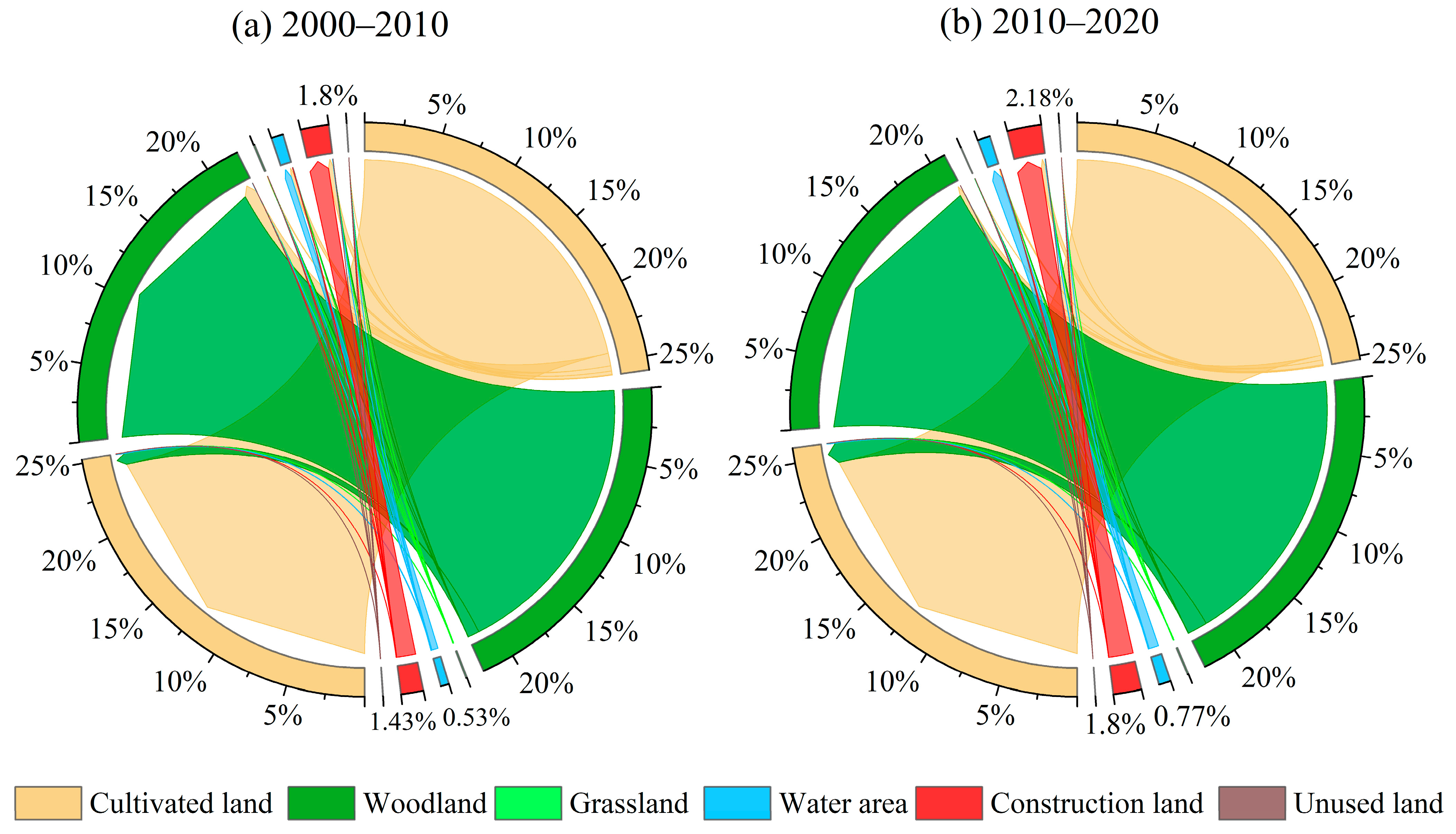
3.1. Analysis of Changes in Landscape Types

Between 2000 and 2020, the structure of landscape types in Harbin remained largely unchanged (Table 5). The two main landscape categories in the study area, cultivated land and woodland, made up over 90% of the overall area, with cultivated land accounting for roughly 50% of the total. The other landscape types, listed in descending order of coverage, were construction land, water bodies, grassland, and unused land. Cultivated land, water area, and building land all showed an overall tendency of expansion over the course of the 20 years. The area of construction land and water area grew consistently, expanding by 798.63 km2 and 296.62 km2, respectively, with their proportions rising by 1.5% and 0.56%. Cultivated land increased the least among them, exhibiting a “V-shaped” fluctuation pattern that saw a fall followed by an increase. For this, 94.69 km2 more land was under cultivation overall at the end of the research period. Woodland, grassland, and unused land showed an overall decline. The unused land had the smallest proportion, consistently remaining below 1%. The woodland area initially increased slightly from 44.15% to 44.29% but subsequently declined to 42.01% by 2020. Grassland remained relatively stable at 0.12% from 2000 to 2010, but its proportion decreased to 0.04% in 2020.
To show patterns of landscape shift, the land use transfer matrix was depicted (Figure 2). During the two periods, the total landscape transition areas in Harbin were 2770.17 km2 and 2543.50 km2, respectively, with the predominant changes occurring between forest land and cultivated land. The primary causes of the decline in arable land between 2000 and 2010 were its conversion to building and forest land, which accounted for 23.58% and 57.78% of the total loss of arable land, respectively. From 2010 to 2020, forest land experienced the largest conversion, primarily transitioning into cultivated land. Since grassland and construction land occupied relatively small proportions, their corresponding flow lines in the land use transition visualization were also thinner.

3.2. Spatiotemporal Analysis of LER Changes

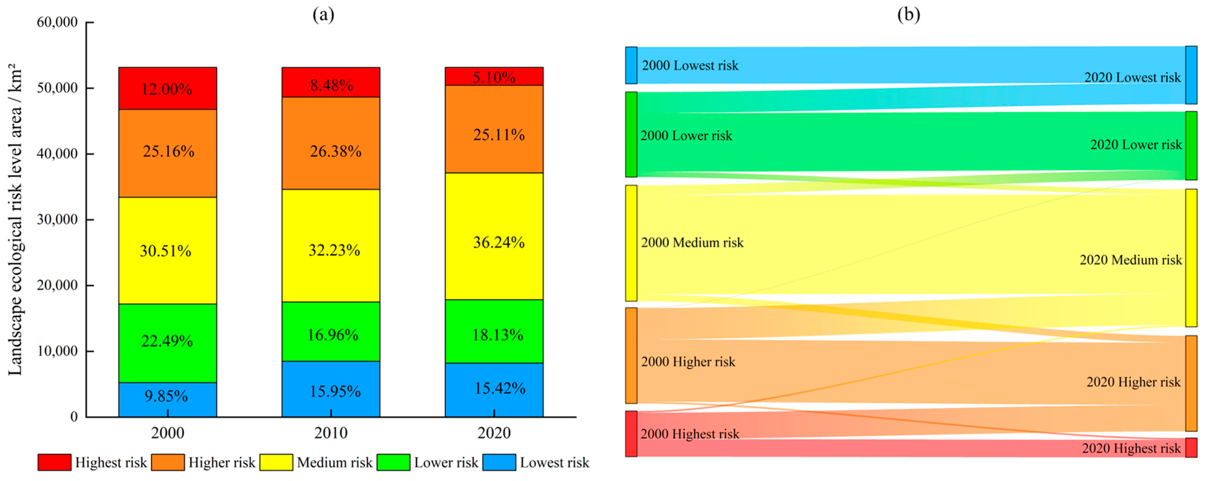
3.2.1. Temporal Evolution Characteristics of LER

Using the natural breaks approach, the LERI for each year was divided into five levels: lowest risk (Ui < 0.0280), lower risk (0.0280 ≤ Ui < 0.0398), medium risk (0.0398 ≤ Ui < 0.0493), higher risk (0.0493 ≤ Ui < 0.0571), and highest risk (Ui ≥ 0.0571). Furthermore, each risk level’s area and proportion were determined (Figure 3a).
Relatively little variation in LER was indicated by the average ERI values in Harbin for 2000, 2010, and 2020, which were 0.0436, 0.0429, and 0.0423, respectively. However, the overall risk level has been gradually decreasing, remaining within the moderate-risk category. Between 2000 and 2010, the lowest risk area expanded by 3240.72 km2, with its proportion rising from 9.85% to 15.95%, indicating a significant expansion. The proportions of the medium-risk and higher-risk areas increased by 910.03 km2 and 647.96 km2, respectively, with their shares rising by 1.72% and 1.23%, respectively. The highest-risk and lower-risk areas showed a declining trend, with their proportions decreasing by 5.53% and 3.52%, respectively. Therefore, the overall LER in Harbin exhibited a declining trend from 2000 to 2010. From 2010 to 2020, the continued reduction in the highest risk areas and the continuous expansion of the lowest risk areas contributed to a further decline in the mean ERI value. The percentage of Harbin’s greatest risk areas fell from 12% to 5.1% overall between 2000 and 2020, while higher risk areas saw a minor decline of less than 1%. In the meantime, the percentage of places with the lowest risk rose from 9.85% to 15.42%. These findings indicate that LER in Harbin has been declining over this period, showing an overall improving trend.
To better examine the changing characteristics of landscape areas under varying risk levels, the area transfer matrix was shown (Figure 3b). From the transition patterns, the conversion of landscape risk levels in Harbin from 2000 to 2020 primarily occurred between adjacent risk levels. The total area where risk levels increased was 1965.02 km2, mainly occurring in transitions from lower to medium risk (744.97 km2), medium to higher risk (966.37 km2), and higher to highest risk (247.86 km2). In contrast, transitions from lowest to lower, lower to higher, and medium to highest risk zones were minimal, each covering less than 5 km2. The total area where risk levels decreased was 12,618.23 km2, mainly involving transitions from lower to lowest, medium to lower, higher to medium, and highest to higher- and medium-risk zones. Overall, from 2000 to 2020, Harbin’s LER has shown an improving trend.

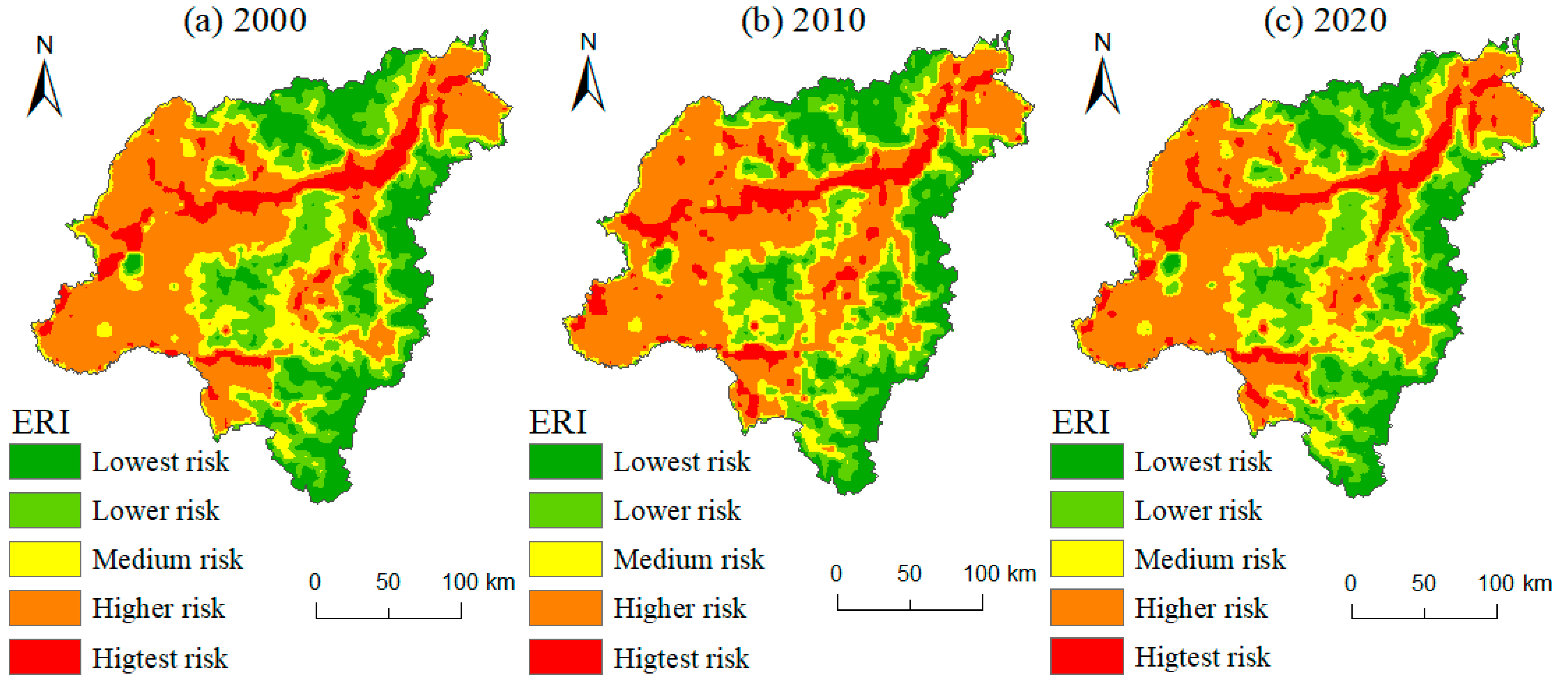
3.2.2. Spatial Evolution Characteristics of LER

Spatiotemporal analysis revealed pronounced spatial heterogeneity in Harbin’s tri-phase LER patterns, demonstrating a cardinal-directional differentiation pattern characterized by west-high-east-low and north-high-south-low risk gradients (Figure 4). The research area’s northern and southeast borders are primarily home to the lowest-risk locations. These zones are characterized by forest-dominated landscapes, elevated topography, minimal anthropogenic construction land, low landscape fragmentation, and well-preserved ecological integrity. Conversely, remaining low-risk zones predominantly occur in built-up landscapes, particularly within peri-urban transition areas connecting Daowai, Daoli, Xiangfang, and Nangang districts. Despite elevated anthropogenic pressure, these areas demonstrate enhanced stability through post-development landscape stabilization, ecological homogenization, and reduced susceptibility to external perturbations. Medium-risk zones primarily manifest as peripheral transitional belts encircling lower-risk core areas, exhibiting spatial configuration patterns consistent with risk gradient attenuation principles. Medium-risk zones are predominantly concentrated in western agricultural hinterlands dominated by croplands, with significant distribution across Bayan County, Hulan District, and Shuangcheng District. These areas exhibit intensified landscape ecological risks where sustained anthropogenic reclamation has driven heightened land-use intensity and elevated ecological vulnerability. Highest and higher risk zones demonstrate significant spatial convergence adjacent to aquatic systems with elevated landscape vulnerability. These areas exhibit pronounced landscape fragmentation and isolation indices, coupled with diminished resistance to anthropogenic perturbations, rendering them particularly prone to ecological degradation.

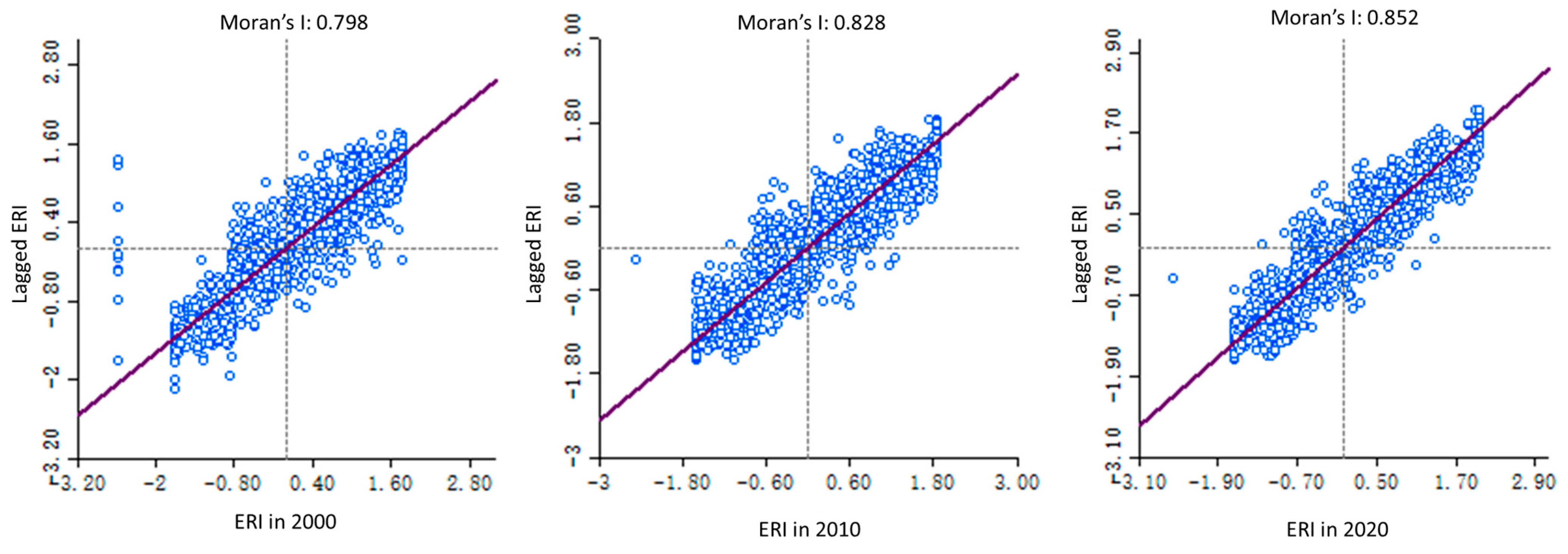
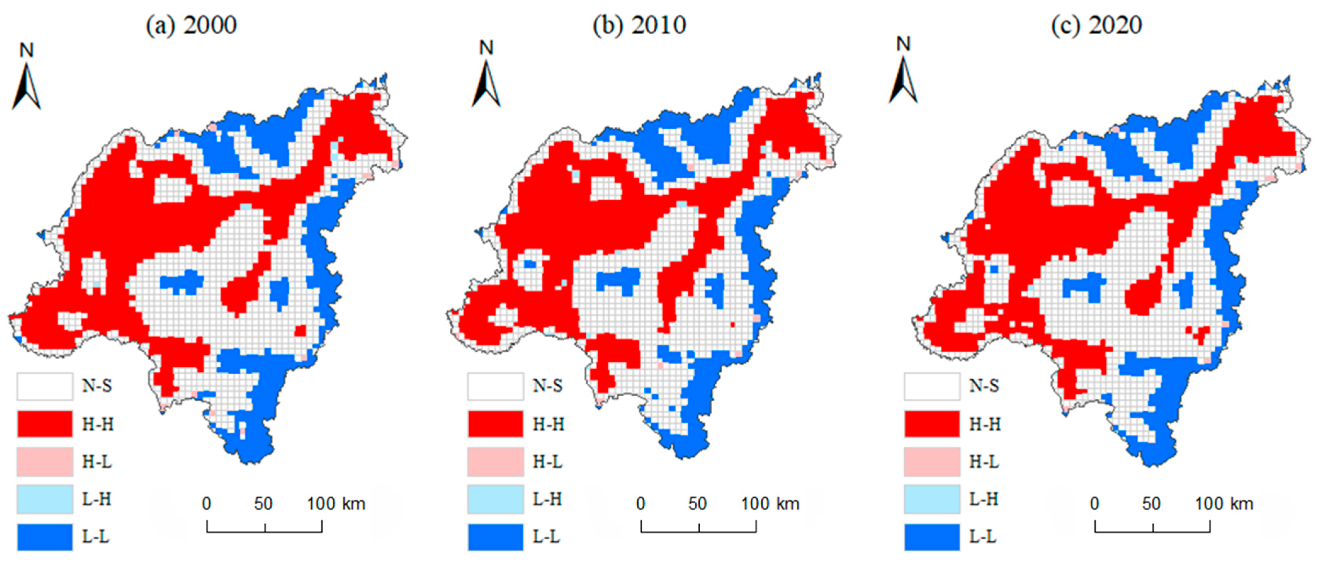
3.3. Spatiotemporal Evolution of the Spatial Aggregation Characteristics of LER

Figure 5, a Moran scatter plot showing ecological risk in landscapes from 2000 to 2020, displays the findings of the use of GeoDa (version 1.20) to calculate the worldwide Moran’s I indices for LER in Harbin City between 2000 and 2020. The corresponding values were 0.798, 0.828, and 0.852. There was a substantial positive geographic correlation in the distribution of LER, as all values were more than 0.5 and the corresponding p-values were less than 0.01. The scatter points show spatially aggregated characteristics of the LER indices in Harbin City, primarily clustering around the regression line. The spatial agglomeration intensity and autocorrelation strength of ecological risk indices initially increased and then decreased over the two-decade period, as evidenced by the worldwide Moran’s I index, which first increased and then declined.
Based on Moran’s I index, generate a LISA clustering graph (Figure 6). Landscape ecological risk in Harbin City demonstrated predominantly “high-high” and “low-low” clustering patterns, while “low-high” and “high-low” clusters exhibited relative spatial dispersion and lower proportional representation. High-high clustering zones exhibited contiguous spatial distribution across western and northeastern sectors, with areal coverage decreasing from 37.46% (2000) to 35.54% (2020), suggesting a progressive reduction in overall low-risk areas within Harbin’s landscape ecological risk profile. “low-low” clustering zones were predominantly concentrated in the eastern sector, demonstrating substantial spatial congruence with low-risk regions, while their areal coverage decreased from 18.32% (2000) to 17.89% (2020). “low-high” and “high-low” clustering patterns exhibited sporadic punctate distributions, with areal proportions consistently remaining below 1% across all study periods. During 2000–2010, “high-high” clustering zones demonstrated moderate expansion, predominantly concentrated in Yanshou County, while “low-low” clusters exhibited gradual contraction, primarily located in Shangzhi City and southern Wuchang City. From 2010 to 2020, “high-high” clustering zones exhibited marked contraction in Yanshou County and Shangzhi City, while the aggregation patterns of landscape ecological risk areas revealed fundamental spatial-structural congruence with their geographic configuration. In ecological risk management strategy formulation, priority implementation of protective measures for “high-high” clustering zones should be instituted to effectively mitigate their potential radiating ecological impacts on adjacent areas.

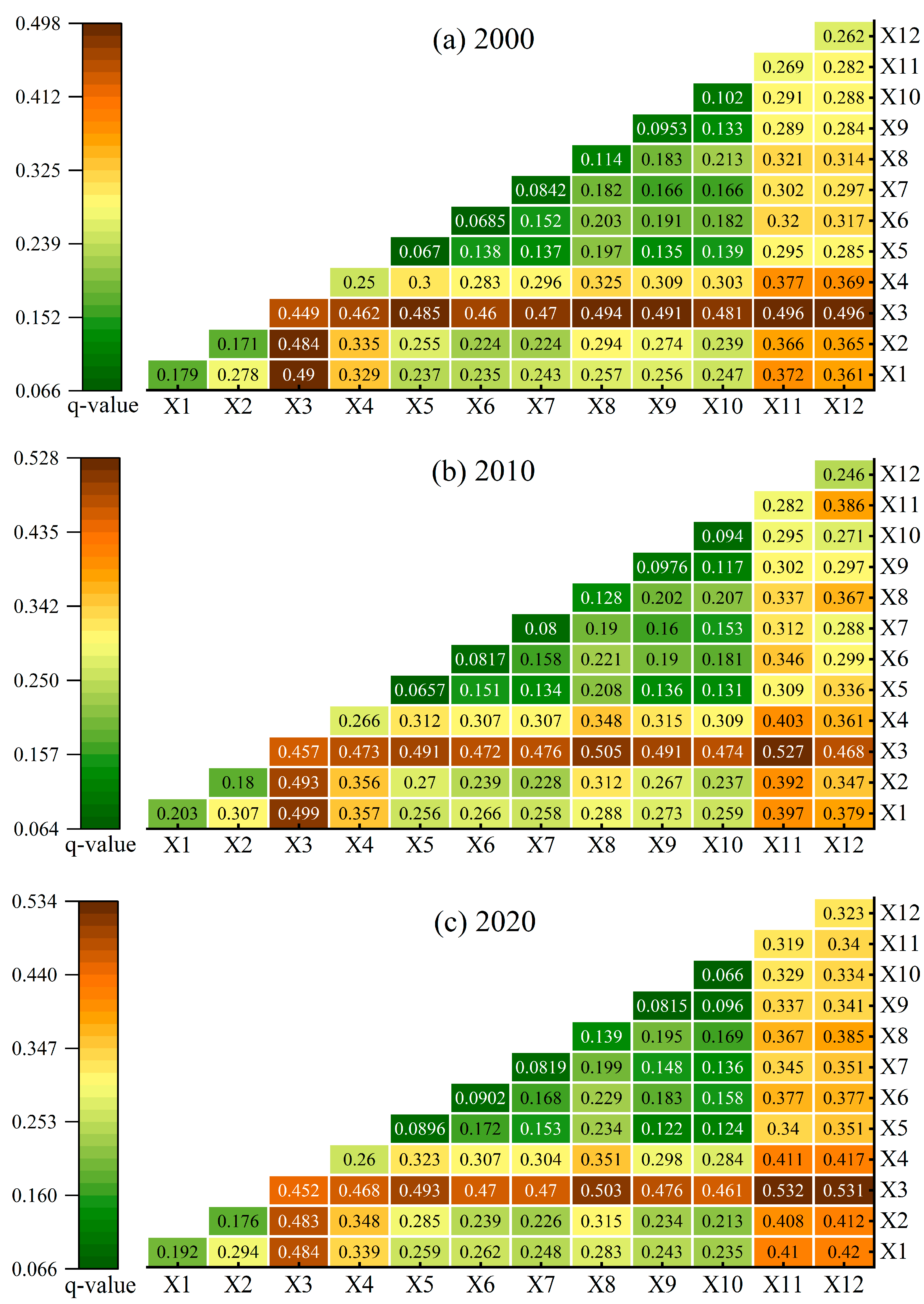
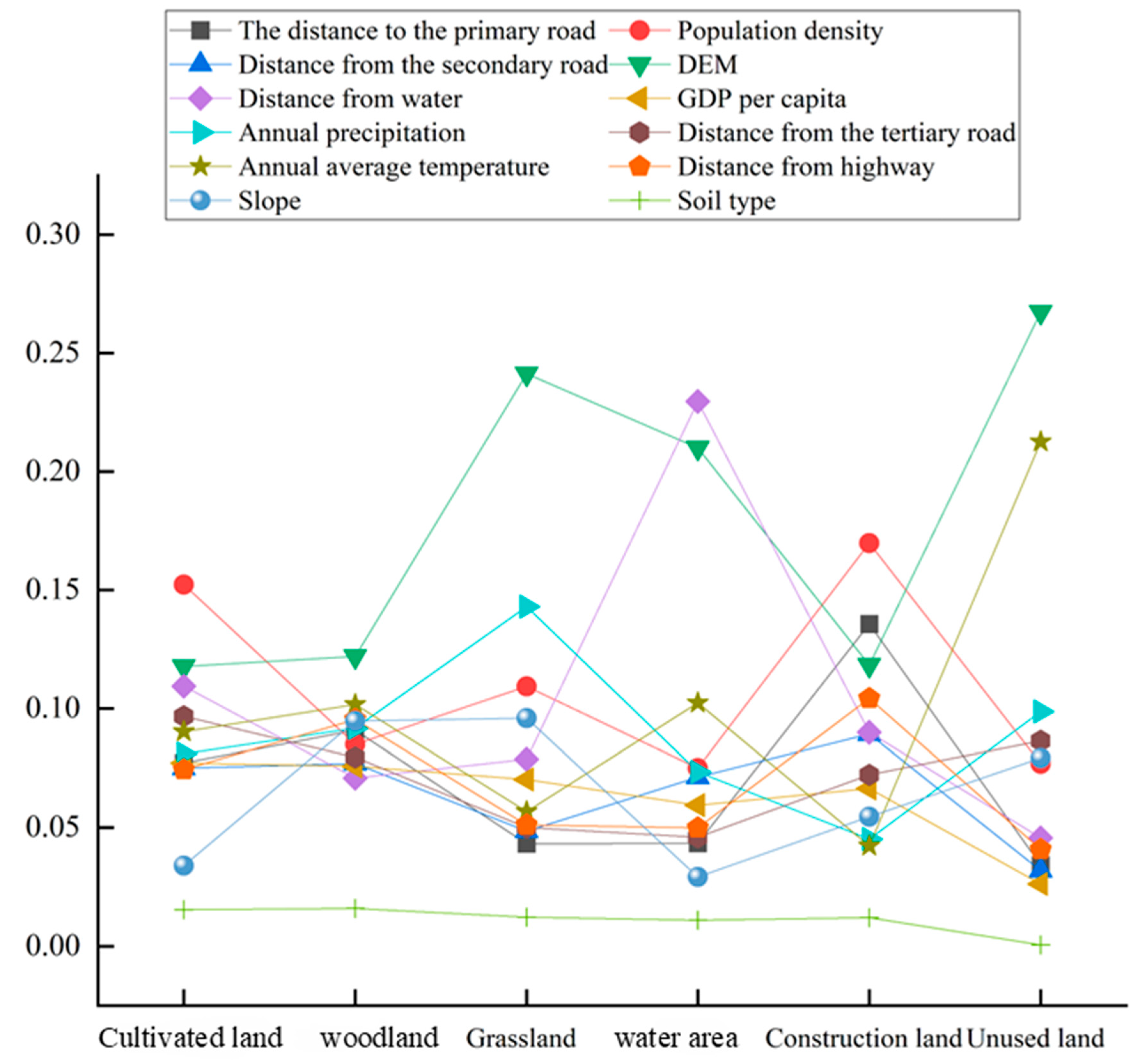
3.4. Analysis of Driving Factors of LER

This study selected 12 independent variables (X) across three dimensions—natural factors, socioeconomic factors, and regional accessibility—spanning the years 2000, 2010, and 2020 to investigate their impact on LER changes (Y). Each variable was discretized using the natural breaks method. The q values of the driving factors for LER, derived from the GeoDetector, are presented in Table 6. The p values for all driving factors across the studied years are 0, indicating that each factor provides a statistically significant explanation for LER. When compared to other components, DEM is the primary driving factor influencing the regional heterogeneity of LER, with the highest average q value, above 0.4. Following DEM, the most influential factors were annual average precipitation, annual average temperature, and slope, with average q values of 0.290, 0.277, and 0.259, respectively. The average q values for distance to primary roads, distance to secondary roads, distance to tertiary roads, population density, and per capita GDP were all below 0.1, indicating that these factors had relatively low explanatory power for LER. This suggests that socioeconomic and regional accessibility factors have a far smaller influence on LER in the research area than do natural factors.
All components’ interaction effects outweighed their separate influences, as seen in Figure 7’s interaction detection results. Furthermore, the interaction detection results consistently showed either bivariate enhancement or nonlinear enhancement over the course of the three periods. This implies that any two factors taken together have a greater impact on LER than any one element alone. Among these interactions, the combination of DEM with other factors exhibited the highest explanatory power, with the interaction effect exceeding 45% in explaining the spatial differentiation of LER. In 2000, the interaction between elevation and both annual average precipitation and annual average temperature was the most significant, with an explanatory power of 49.6% in each case. In 2010 and 2020, the interaction between elevation and annual average precipitation exhibited the highest explanatory power, reaching 52.7% and 53.2%, respectively. Additionally, the interaction between DEM and distance to highways demonstrated strong explanatory power from 2000 to 2020, consistently exceeding 49%. This suggests that the study area’s LER is mostly shaped by the interaction of natural forces. Specifically, the interaction between DEM and annual average precipitation significantly influences the spatiotemporal heterogeneity of LER in Harbin. Natural, social, and regional accessibility variables all work together to produce Harbin’s LER.

3.5. Land Use Simulation and Prediction Under Multiple Scenarios

3.5.1. Land Use Expansion Analysis

For this study, 12 driving factors are chosen by the PLUS model’s LEAS module to model the regional distribution of land use categories in 2030. By incorporating the random forest method, the likelihood of land use growth and the role of different factors in land expansion are further assessed. The results indicate that the driving force analysis’s RMSE values, which are all below 0.45 for various landscape types, illustrate the model’s high accuracy and dependability [58]. Figure 8 illustrates how soil type has a negligible effect on different landscape categories. This is attributed to the balanced distribution of soil types in Harbin, where the demand for soil characteristics does not vary significantly across different land use types. With factor contribution values greater than 0.15, population density significantly affects the distribution of both farmed and constructed land.
The DEM contributes the most to the expansion of woodland, grassland, and unused land, while also playing a significant role in the distribution of water areas. DEM is a key variable in determining landscape types and geomorphological characteristics, as the distribution of woodland, grasslands, and water sources is closely linked to specific terrain conditions. High-altitude areas are more suitable for forest growth, whereas low-altitude areas are more favorable for the distribution of grasslands and water areas.

3.5.2. Analysis of Landscape Change in Harbin Under Multiple Scenarios for 2030

The Kappa coefficient is used in this study to validate accuracy. The land use pattern for 2020 is simulated using the CARS module using land use data from 2000 and 2010, and the results are compared to the real 2020 data. Higher values of the Kappa coefficient, which goes from 0 to 1, indicate better simulation performance. When Kappa > 0.75, the simulated map exhibits a high degree of consistency with the real-world data, suggesting a reliable simulation outcome [19]. The model achieved an overall classification accuracy of 91% and a Kappa coefficient of 0.85, which reflects a high level of agreement between the simulated and actual 2020 land use patterns (Table 7 and Figure 9). Cultivated land and woodland continue to be the most common landscape types in Harbin, notwithstanding minor differences between the scenarios. Under the ND scenario, without considering policy or other human interventions, the trends observed from 2010 to 2020 continue, with the expansion of construction land, water area, and cultivated land, along with the contraction of grassland, unused land, and woodland. Compared to 2020, construction land exhibits the largest increase, rising by 17.15%, while grassland experiences the most significant decline, decreasing by 19.53%. As shown in Figure 10a, construction land expands into the Acheng District, encroaching on a portion of its woodland. Under the CP scenario, cultivated land exhibits the largest increase, with an expansion of 3.27%. Changes in water area and construction land are minimal, while woodland, grassland, and unused land show a decreasing trend. Among them, grassland experiences the most significant reduction, declining by 37.50%, with most of the cultivated land expansion occurring at the expense of grassland. Compared to the natural development scenario, both cultivated land and woodland increase in area, while construction land decreases. This indicates that the scenario effectively constrains construction land expansion and ensures the protection of farmland. Under the CP scenario, compared to 2020, the areas of cultivated land, woodland, and water area all increase, with the water area experiencing a significant expansion of 40.69 km2, representing a 4.73% increase. The remaining land categories decrease to varying degrees, with construction land showing the most substantial reduction, decreasing by 2319.17 km2 or 17.43%. While construction land shrinks, the area of both cultivated land and woods increases in comparison to the ND scenario. This indicates that this scenario provides a certain degree of protection for ecologically valuable land types, reducing the area of construction land and expanding ecological space.

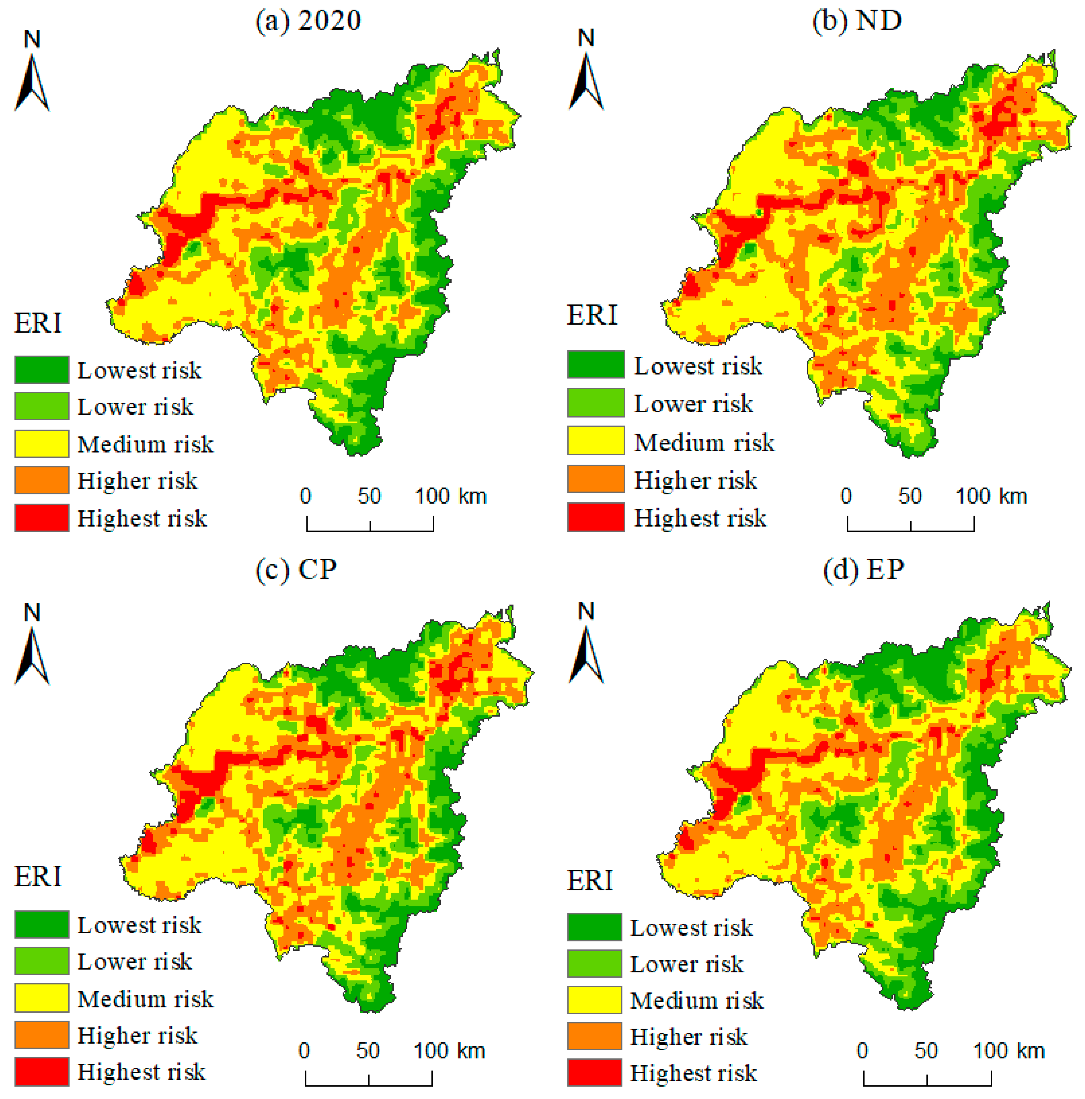
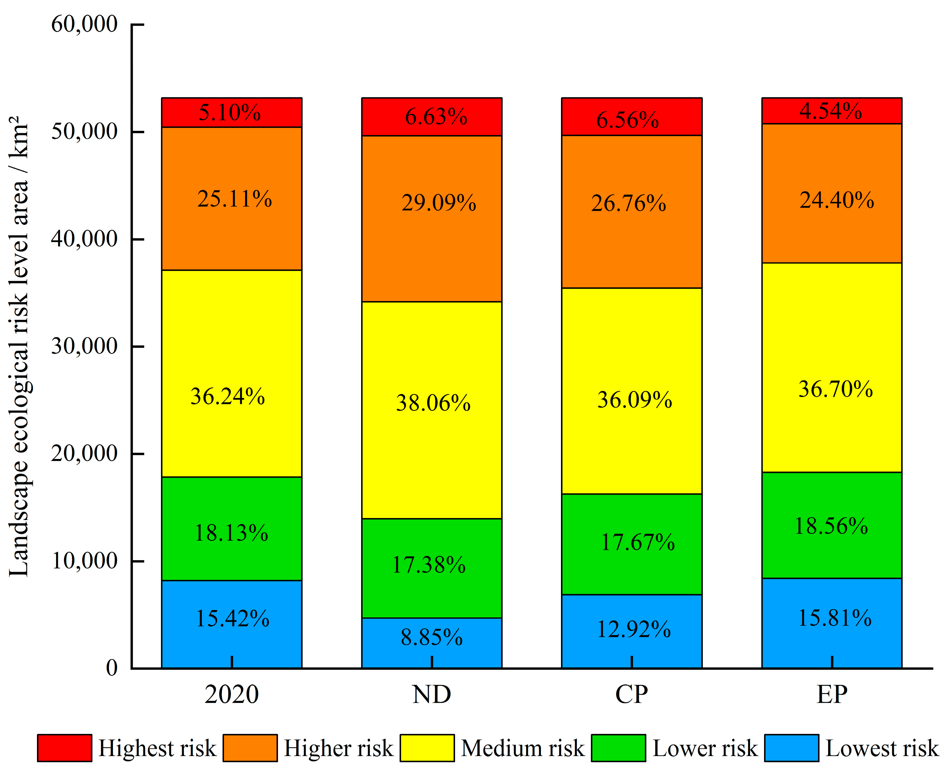
3.5.3. Simulation and Prediction of LER in Harbin Under Multiple Scenarios for 2030

A more thorough examination of Harbin’s LER under several scenarios for 2030 was carried out. By comparing the spatial distribution of LER between 2022 and 2030, the results are presented in Figure 10. The graphic illustrates that, under various scenarios in 2030, the spatial distribution pattern of landscape ecological risk in Harbin is comparable to its historical distribution. With mean ERI values of 0.0446, 0.0434, and 0.0420, respectively, the LER levels in all three situations primarily stay at a moderate level.
Based on the analysis in Figure 11, under the ND scenario, the areas of all LER levels exhibit some variation compared to 2020. The areas of lowest and lower risk regions decrease, with the lowest risk area experiencing a significant reduction of 3494.77 km2 and the lower risk area showing a slight decrease of 401.47 km2. In contrast, the areas of medium, higher, and highest ecological risk regions increase by 968.59 km2, 2114.52 km2, and 812.12 km2, respectively. Overall, the LER in Harbin under the ND scenario in 2030 shows an increasing trend, indicating a deterioration in overall ecological environmental quality. Under the CP scenario, the mean ERI shows a slight decrease compared to 2020.
The areas of lowest, lower, and medium landscape ecological risk regions decrease by 1328.66 km2, 245.41 km2, and 80.63 km2, respectively, with the lowest risk area experiencing the most significant reduction at 16.21%. The areas of the highest LER regions, however, grow by 777.90 km2 and 876.61 km2, respectively. This suggests that under the CP scenario in 2030, the LER in Harbin still exhibits an increasing trend. This may be attributed to cultivated land protection policies prompting the expansion of construction land into ecological land, thereby exacerbating landscape fragmentation.
Under the EP scenario, the LER levels show slight changes compared to 2020. While the areas of higher- and highest-risk regions decline, the areas of lowest-, lower-, and medium-risk regions grow. Specifically, the total increase in the lowest and lower risk areas amounts to 433.85 km2, while the total reduction in the highest and higher risk areas is 680.43 km2. This scenario leads to an improvement in ecological environmental quality, which is beneficial for maintaining ecological balance and enhancing ecological carrying capacity.
The EP scenario contains the largest percentage of the lowest-risk areas among the three scenarios (15.81%), followed by the CP scenario (12.92%). With the lowest-risk locations showing a clustered distribution in the northern part of Tonghe County, the northeastern part of Shangzhi City, and the southeast half of Wuchang City, the ND scenario has the smallest proportion (8.85%). Under both the EP and CP scenarios, the proportions of relatively lower risk and highest risk areas are relatively similar, ranging between 17–18% and 6–7%, respectively. The highest risk areas are concentrated in a contiguous pattern at the junctions of Hulan District, Daowai District, and Songbei District, as well as the boundary between Songbei District and Daoli District. Under the CP scenario, the proportion of medium-risk areas is the smallest at 36.09%, while under the EP scenario, it is the largest at 38.06%. These areas are primarily distributed in Shuangcheng District, Hulan District, Bayan County, the northwestern part of Wuchang City, and the southern part of Tonghe County. Under the EP scenario, the highest risk area is the smallest, while the lowest ecological risk area is the largest. This is mostly because of improved EP regulations, which limit the growth of agricultural and building land while creating water-saving zones, protecting the stability of the ecology.

4. Discussion

4.1. Spatiotemporal Analysis of LER

Over the past 20 years, building land, woodland, and cultivated land have continued to be Harbin’s three primary land use types. According to the results of the pertinent literature, cultivated land and building land have increased while woodland has decreased [59,60]. According to Zhang Xinyang et al.’s study, Harbin’s predominant landscape types are woodland and cultivated land, with the area of building land having significantly increased. However, some differences exist between the study results. For instance, Zhang Xinyang et al. propose that the cultivated land area first increased and then reduced, whereas this analysis reveals that it first decreased and then increased. There may be some variation in the results due to this mismatch, which could be explained by variations in the sources of land use data. Such minor variations are reasonable and expected.
According to this study, there was a downward trend in Harbin’s landscape ecological risk index between 2000 and 2020. This is mostly because, during the first ten years, measures like the Natural Forest Protection Project and the Grain-for-Green Program reduced the amount of land under cultivation and increased the amount of forest and grassland regions. These measures contributed to reducing regional landscape ecological risk. After 2010, ecological deterioration resulted from the quick growth of the tourism sector and the rapid expansion of cities. In reaction, the government placed significant emphasis on ecological protection, formulating comprehensive land management policies and ecological security regulations. These measures have improved the ecological environment’s quality to some extent, which has reduced LER. There is a strong correlation between Harbin’s natural geographical features and the spatial distribution pattern of LER [61,62]. Topographical factors fundamentally shape the landscape pattern and profoundly influence the spatiotemporal distribution of LER. The forested areas along the northern and southeastern boundaries of the study area, characterized by higher elevations and extensive vegetation cover, exhibit a contiguous forest landscape. Over the years of development, the landscape structure has stabilized, resulting in a more resilient ecosystem and lower LER. As elevation decreases and the terrain becomes more level, the region becomes increasingly affected by human activities. With sporadic patches of grassland and vacant land, vast tracts of forest land are progressively being turned into farmland. This leads to higher landscape fragmentation, increased ecological vulnerability, and elevated landscape ecological risk. As elevation further decreases, the dominant landscape type transitions to large-scale construction land. Due to planned development and concentrated construction landization, landscape fragmentation and disturbance levels are relatively low, leading to a reduction in LER.
Harbin’s LER trend stayed steady between 2000 and 2020, with “low-low clusters” mostly dispersed in the lowest risk areas and “high-high clusters” concentrated in the highest risk areas. This suggests that LER’s geographic clustering features match its spatial distribution, which is in line with results from similar research [63]. Future land use planning should prioritize places with the highest risk, and the appropriate authorities should improve ecological risk management and control in these areas.

4.2. Analysis of Driving Factors of LER

Through this study of the spatiotemporal differentiation drivers of LER in Harbin, it was found that DEM is the primary driving factor influencing landscape ecological risk changes, while annual precipitation is the second most dominant factor. DEM is closely associated with a number of ecological, meteorological, and hydrological issues in addition to representing geomorphological features. Since landscape distribution is to some extent constrained by topography, DEM has a significant impact on LER. The amount of precipitation has a significant impact on vegetation growth, and the degree of vegetation development also affects the ecosystem’s stability. The results of the interaction detection show that LER is more strongly impacted by the combined influence of DEM and yearly precipitation. Instead of being determined by a single cause, the LER in Harbin is the outcome of the synergistic combination between natural, socioeconomic, and regional accessibility factors. Natural factors are the primary driving forces behind the spatiotemporal differentiation of LER, which is consistent with related research findings [64]. The explanatory power increases significantly when natural and human factors interact, indicating that human activity also has a significant influence on LER.

4.3. Analysis of LER Changes Under Different Scenarios

According to the multi-scenario land use pattern and LER projection results for Harbin, the ecological conservation scenario exhibits the smallest fraction of highest and higher risk areas in comparison to the natural development and cultivated land preservation scenarios. This suggests a decrease in LER, which is in line with results from prior research [65]. This is because there is less chance of ecological land like woodland and grassland being converted in this scenario, which improves landscape connectedness and lessens landscape fragmentation. As a result, ecosystem stability is maintained, leading to a reduction in LER. Under the cultivated land protection scenario, prioritizing the preservation of cultivated land and restricting its conversion to other land types increases landscape fragmentation and reduces ecosystem connectivity, ultimately leading to a rise in LER. Moreover, urban expansion plays a critical role in both current and future land use changes and has become a key driver affecting areas of high ecological value. Under the ND scenario in this study, Shuangcheng District in Harbin exhibits a continuous expansion of construction land, leading to a reduction in ecological land types such as forest and grassland, an increase in landscape fragmentation, and a decline in ecosystem connectivity. This rapid transformation in spatial land structure significantly elevates the level of regional landscape ecological risk, particularly in urban fringe areas and ecologically sensitive zones. In addition, urban expansion is often accompanied by infrastructure development and population concentration, which pose potential disturbances to ecological functional areas and increase the vulnerability of regional ecosystems.

4.4. Recommendations for Future Development

Based on the current status of the field and the results of the LER evaluation in different scenarios, the following recommendations are made for different risk levels: (1) For the lowest and lower ecological risk areas, which are primarily located in forested regions, it is essential to continue strengthening forest resource protection based on existing policy measures. Additionally, strict precautions should be taken to prevent forest fires, minimizing disturbances to the landscape ecosystem. (2) For the highest and higher ecological risk areas, which are primarily distributed near water bodies, it is recommended that relevant authorities strengthen water environment monitoring and early warning systems, improve wastewater treatment facilities, and enhance water pollution prevention and control measures to mitigate the existing high-risk conditions. (3) For medium-risk areas, which are primarily composed of cultivated land, strict enforcement of the cultivated land protection red line should be ensured to promote the high-quality development of basic farmland, thereby reducing landscape fragmentation. Regular monitoring of soil pollution should be conducted to ensure the ecological security of farmland. For damaged farmland, timely post-disaster land restoration and reclamation efforts should be carried out to maintain agricultural sustainability.

4.5. Limitations and Future Directions

This study presents certain limitations that need to be acknowledged: (1) The landscape vulnerability index in the LER assessment is derived from expert scoring, which introduces a degree of subjectivity. To further enhance the landscape ecological risk model and increase the computations’ accuracy, future studies should include more objective indicators (2). The selection of driving factors was limited by data availability, resulting in the exclusion of potentially influential factors such as governmental policy interventions, socio-economic dynamics, and natural disasters. As a consequence, the current study analyzed only 12 measurable driving factors, potentially causing discrepancies between the predicted scenarios and actual ecological conditions. Future research should adopt a more comprehensive and integrated modeling approach, incorporating a wider range of risk sources and employing advanced modeling techniques, such as machine learning algorithms, to capture the complex interplay of multiple driving factors. (3) This study categorizes land use types into six primary categories (e.g., cultivated land, woodland, and grassland) but lacks analysis of more detailed secondary and tertiary classifications. A more sophisticated land use classification scheme should be used in future studies to improve the precision of regional LER evaluations. (4) Future research could incorporate higher-resolution remote sensing data to enhance the spatial precision of ecological risk assessments, especially for urban or peri-urban areas.

5. Conclusions

This study explored the spatiotemporal evolution, spatial patterns, driving mechanisms, and future trends of LER in Harbin, China, from 2000 to 2020. The results indicated that the LERI in Harbin experienced a gradual decline over the study period, with values shifting from 0.0436 in 2000 to 0.0423 in 2010 and further decreasing to 0.2486 in 2020. The overall risk level remained predominantly medium. Spatially, ecological risk exhibited a clear distribution pattern—higher in the west and north and lower in the east and south. The lowest-risk areas were found in high-altitude forest regions, while medium-risk areas were mostly distributed across cultivated lands, and the highest-risk zones were concentrated near water bodies.
Spatial autocorrelation analysis showed that Moran’s I remained above 0.5 throughout the two decades, indicating strong spatial clustering. “high-high” and “low-low” clusters were the dominant patterns. Between 2000 and 2010, “high-high” clusters expanded, while “low-low” clusters shrank; from 2010 to 2020, the “high-high” areas contracted, whereas the “low-low” clusters remained stable.
GeoDetector analysis identified DEM as the most influential single driving factor for LER, with the interaction between DEM and annual precipitation demonstrating the highest explanatory power among factor combinations. These findings emphasize the need for integrated consideration of multiple natural variables in ecological management and land use planning.
The PLUS model simulation revealed that from 2000 to 2020, cultivated land and construction land expansion were mainly driven by population density, while the distribution of woodland, grassland, water, and unused land was more influenced by topographical factors.
Based on scenario simulations for the year 2030, the dominant landscape types in Harbin are forecasted to remain cultivated land and forest land. The spatial distribution patterns of ecological risk under all three scenarios are projected to be similar to those in 2020. Among the scenarios, the ecological priority scenario is expected to result in the smallest area of highest risk zones and the largest area of lowest risk zones. This forecasted outcome suggests that prioritizing ecological conservation can better align with Harbin’s long-term development goals and contribute to a more balanced and resilient ecological security pattern.

Author Contributions

Conceptualization, Y.L. and J.L.; methodology, Y.L.; software, Y.L.; validation, Y.Z. and C.W.; formal analysis, Y.L.; investigation, Y.L. and J.L.; resources, Y.L. and J.L.; data curation, C.W.; writing—original draft preparation, Y.Z.; writing—review and editing, Y.L. and J.L.; visualization, C.W.; supervision, J.L.; project administration, Y.L. and J.L.; funding acquisition, J.L. All authors have read and agreed to the published version of the manuscript.

Funding

This research was funded by the National Natural Science Foundation of China (41977411), the Science and Technology Development Program of Jilin Province (YDZJ202501ZYTS492), the Jilin Provincial Department of Education (JJKH20240563CY), and the Social Science Foundation of Jilin Province (2022B40).

Data Availability Statement

Data are contained within the article.

Conflicts of Interest

The authors declare that there are no conflicts of interest.

References

  1. Amato, F.; Pontrandolfi, P.; Murgante, B. Supporting planning activities with the assessment and the prediction of urban sprawl using spatio-temporal analysis. Ecol. Indic. 2015, 30, 365–378. [Google Scholar] [CrossRef]
  2. Dewan, A.M.; Yamaguchi, Y. Land use and land cover change in Greater Dhaka, Bangladesh: Using remote sensing to promote sustainable urbanization. Appl. Appl. Geogr. 2009, 29, 390–401. [Google Scholar] [CrossRef]
  3. Zhang, Y.; Li, Y.Z.; Lv, J.; Wang, J.; Wu, Y. Scenario simulation of ecological risk based on land use/cover change—A case study of the Jinghe county, China. Ecol. Indic. 2021, 131, 108176. [Google Scholar] [CrossRef]
  4. Kayumba, P.M.; Chen, Y.; Mind’je, R.; Mindje, M.; Li, X.; Maniraho, A.P.; Umugwaneza, A.; Uwamahoro, S. Geospatial land surface-based thermal scenarios for wetland ecological risk assessment and its landscape dynamics simulation in Bayanbulak Wetland, Northwestern China. Landsc. Ecol. 2021, 36, 1699–1723. [Google Scholar] [CrossRef]
  5. United Nations. Transforming Our World: The 2030 Agenda for Sustainable Development; United Nations: New York, NY, USA, 2015. [Google Scholar]
  6. Convention on Biological Diversity. Kunming-Montreal Global Biodiversity Framework—COP 15 Decision 15/4; CBD Secretariat: Montreal, QC, Canada, 2022. [Google Scholar]
  7. Forman, R.T.T. Land Mosaics: The Ecology of Landscapes and Regions; Cambridge University Press: Cambridge, UK, 1995. [Google Scholar]
  8. Rescia, A.J.; Willaarts, B.A.; Schmitz, M.F.; Aguilera, P.A. Changes in land uses and management in two Nature Reserves in Spain: Evaluating the social–ecological resilience of cultural landscapes. Landsc. Urban Plan. 2010, 98, 26–35. [Google Scholar] [CrossRef]
  9. Romero-Ruiz, M.H.; Flantua, S.G.A.; Tansey, K.; Berrio, J.C. Landscape transformations in savannas of northern South America: Land use/cover changes since 1987 in the Llanos Orientales of Colombia. Appl. Geogr. 2012, 32, 766–776. [Google Scholar] [CrossRef]
  10. Mandal, M.; Chatterjee, N.D. Forest landscape and its ecological quality: A stepwise spatiotemporal evaluation through patch-matrix model in Jhargram District, West Bengal State, India. Reg. Sustain. 2021, 2, 164–176. [Google Scholar] [CrossRef]
  11. Peter, C. Ecological risk assessment: Risk for what? How do we decide? Ecotoxicol. Environ. Saf. 1998, 40, 15–18. [Google Scholar]
  12. Suter, G.W. Ecological Risk Assessment; CRC Press: Boca Raton, FL, USA, 2006. [Google Scholar]
  13. Ayre, K.K.; Landis, W.G. A Bayesian approach to landscape ecological risk assessment applied to the upper Grande Ronde watershed, Oregon. Hum. Ecol. Risk Assess. Int. J. 2012, 18, 946–970. [Google Scholar] [CrossRef]
  14. Proshad, R.; Kormoker, T.; Islam, S. Distribution, source identification, ecological and health risks of heavy metals in surface sediments of the Rupsa River, Bangladesh. Toxin Rev. 2021, 40, 77–101. [Google Scholar] [CrossRef]
  15. Omar, H.; Cabral, P. Ecological risk assessment based on land cover changes: A case of Zanzibar (Tanzania). Remote Sens. 2020, 12, 3114. [Google Scholar] [CrossRef]
  16. Yanes, A.; Botero, C.M.; Arrizabalaga, M.; Vásquez, J.G. Methodological proposal for ecological risk assessment of the coastal zone of Antioquia, Colombia. Ecol. Eng. 2019, 130, 242–251. [Google Scholar] [CrossRef]
  17. Lin, Y.Y.; Hu, X.S.; Zheng, X.X.; Hou, X.Y.; Zhang, Z.X.; Zhou, X.N.; Qiu, R.Z.; Lin, J.G. Spatial variations in the relationships between road network and landscape ecological risks in the highest forest coverage region of China. Ecol. Indic. 2019, 96, 392–403. [Google Scholar] [CrossRef]
  18. Harwell, M.A.; Cooper, W.; Flaak, R. Prioritizing ecological and human welfare risks from environmental stresses. Environ. Manag. 1992, 16, 451–464. [Google Scholar] [CrossRef]
  19. Lin, X.; Wang, Z.T. Landscape ecological risk assessment and its driving factors of multi-mountainous city. Ecol. Indic. 2023, 146, 109823. [Google Scholar] [CrossRef]
  20. Wei, Y.L.; Zhou, P.Y.; Zhang, L.Q.; Zhang, Y. Spatio-temporal evolution analysis of land use change and landscape ecological risks in rapidly urbanizing areas based on Multi-Situation simulation—A case study of Chengdu Plain. Ecol. Indic. 2024, 166, 112245. [Google Scholar] [CrossRef]
  21. Li, S.K.; Tu, B.; Zhang, Z.; Wang, L.; Zhang, Z.; Chen, X.Q.; Wang, Z.Z. Exploring new methods for assessing landscape ecological risk in key basin. J. Clean. Prod. 2024, 461, 142633. [Google Scholar] [CrossRef]
  22. Wang, S.S.; Tan, X.; Fan, F.L. Landscape Ecological Risk Assessment and Impact Factor Analysis of the Qinghai-Tibetan Plateau. Remote Sens. 2022, 14, 472619. [Google Scholar] [CrossRef]
  23. Zang, Z.; Zou, X.Q.; Zuo, P.; Song, Q.C.; Wang, C.L.; Wang, J.J. Impact of landscape patterns on ecological vulnerability and ecosystem service values: An empirical analysis of Yancheng Nature Reserve in China. Ecol. Indic. 2017, 72, 142–152. [Google Scholar] [CrossRef]
  24. Gan, L.; Halik, Ü.; Shi, L.; Welp, M. Ecological risk assessment and multi-scenario dynamic prediction of the arid oasis cities in northwest China from 1990 to 2030. Stoch. Environ. Res. Risk Assess. 2023, 37, 3099–3115. [Google Scholar] [CrossRef]
  25. Si, Q.; Fan, H.R.; Dong, W.M.; Liu, X.P. Landscape ecological risk assessment and prediction for the Yarkant River Basin, Xinjiang, China. Arid. Zone Res. 2024, 41, 684–696. [Google Scholar]
  26. Hou, M.J.; Ge, J.; Gao, J.L.; Meng, B.P.; Li, Y.C.; Yin, J.P.; Liu, J.; Feng, Q.S.; Liang, T.G. Ecological risk assessment and impact factor analysis of alpine wetland ecosystem based on LUCC and boosted regression tree on the Zoige Plateau, China. Remote Sens. 2022, 12, 368. [Google Scholar] [CrossRef]
  27. Liu, K.X.; Wang, D.M.; Wei, Y.S.; Chang, G.L. Spatio-temporal evolution trend of multi-scale landscape ecological risk in Miyun Reservoir watershed. Acta Ecol. Sin. 2023, 43, 105–117. [Google Scholar]
  28. Li, B.J.; Du, X.Y.; Zhu, S. Multi-scenario simulation of landscape ecological risk assessment in Huaihai Economic Zone. China Environ. Sci. 2024, 45, 2112–2121. [Google Scholar]
  29. Karimian, H.; Zou, W.; Chen, Y.; Xia, J.; Wang, Z. Landscape ecological risk assessment and driving factor analysis in Dongjiang river watershed. Chemosphere 2022, 307, 135835. [Google Scholar] [CrossRef]
  30. Yang, N.J.; Zhang, T.; Li, J.Z.; Feng, P.; Yang, N. Landscape ecological risk assessment and driving factors analysis based on optimal spatial scales in Luan River Basin, China. Ecol. Indic. 2024, 169, 112821. [Google Scholar] [CrossRef]
  31. Xie, H.; Wang, P.; Huang, H. Ecological Risk Assessment of Land Use Change in the Poyang Lake Eco-economic Zone, China. Int. J. Environ. Res. Public Health 2013, 10, 328–346. [Google Scholar] [CrossRef] [PubMed]
  32. Wang, Z.; Guo, M.; Zhang, D.; Chen, R.; Xi, C.; Yang, H. Coupling the Calibrated GlobalLand30 Data and Modified PLUS Model for Multi-Scenario Land Use Simulation and Landscape Ecological Risk Assessment. Remote Sens. 2023, 15, 5186. [Google Scholar] [CrossRef]
  33. Peng, L.; Dong, B.; Wang, P.; Sheng, S.W.; Sun, L.; Fang, L.; Li, H.R.; Liu, L.P. Research on ecological risk assessment in land use model of Shengjin Lake in Anhui province, China. Environ. Geochem. Health 2019, 41, 2665–2679. [Google Scholar] [CrossRef]
  34. Wang, H.; Liu, X.M.; Zhao, C.Y.; Chang, Y.P.; Liu, Y.Y.; Zang, F. Spatial-temporal pattern analysis of landscape ecological risk assessment based on land use/land cover change in Baishuijiang National nature reserve in Gansu Province, China. Ecol. Indic. 2021, 124, 107454. [Google Scholar] [CrossRef]
  35. Molinos, J.G.; Takao, S.; Kumagai, N.H.; Poloczanska, E.S.; Burrows, M.T.; Fujii, M.; Yamano, H. Improving the interpretability of climate landscape metrics: An ecological risk analysis of Japan’s Marine Protected Areas. Glob. Chang. Biol. 2017, 23, 4440–4452. [Google Scholar] [CrossRef] [PubMed]
  36. Mondal, B.; Sharma, P.; Kundu, D.; Bansal, S. Spatio-temporal assessment of landscape ecological risk and associated drivers: A case study of Delhi. Environ. Urban. Asia 2021, 12, S85–S106. [Google Scholar] [CrossRef]
  37. Cui, B.; Zhang, Y.; Wang, Z.; Gu, C.; Liu, L.; Wei, B.; Gong, D.; Rai, M.K. Ecological Risk Assessment of Transboundary Region Based on Land-Cover Change: A Case Study of Gandaki River Basin, Himalayas. Land 2022, 11, 638. [Google Scholar] [CrossRef]
  38. Xia, Y.; Li, J.; Li, E.; Liu, J. Analysis of the Spatial and Temporal Evolution and Driving Factors of Landscape Ecological Risk in the Four Lakes Basin on the Jianghan Plain, China. Sustainability 2023, 15, 13806. [Google Scholar] [CrossRef]
  39. Li, S.N.; Zhao, X.Q.; Pu, J.W.; Miao, P.P.; Wang, Q.; Tan, K. Optimize and control territorial spatial functional areas to improve the ecological stability and total environment in karst areas of southwest China. Land Use Policy 2021, 100, 104940. [Google Scholar] [CrossRef]
  40. Darvishi, A.; Yousefi, M.; Marull, J. Modelling landscape ecological assessments of land use and cover change scenarios. Application to the Bojnourd Metropolitan Area (NE Iran). Land Use Policy 2020, 99, 105098. [Google Scholar] [CrossRef]
  41. Peng, J.; Hu, X.X.; Wang, X.Y.; Meersmans, J.; Liu, Y.X.; Qiu, S.J. Simulating the impact of Grain-for-Green Programme on ecosystem services trade-offs in Northwestern Yunnan, China. Ecosyst. Serv. 2019, 39, 100998. [Google Scholar] [CrossRef]
  42. Li, X.J.; Che, L.G.; Hu, B.Q. Spatio-temporal difference analysis of carbon storage in Beihai secosystem based on FLUS-InVEST models. Bull. Surv. Mapp. 2023, 6, 117–123. [Google Scholar]
  43. Liang, X.; Guan, Q.F.; Clarke, K.C.; Liu, S.S.; Wang, B.Y.; Yao, Y. Understanding the drivers of sustainable land expansion using a patch-generating land use simulation (PLUS) model: A case study in Wuhan, China. Comput. Environ. Urban Syst. 2021, 85, 101569. [Google Scholar] [CrossRef]
  44. Xu, X.X.; Peng, Y.L.; Qin, W.J. Simulation, prediction and driving factor analysis of ecological risk in Savan District, Laos. Front. Environ. Sci. 2022, 10, 1058792. [Google Scholar]
  45. Tian, Y.D.; Zhao, X.C. Simulation of construction land expansion and carbon emission response analysis of Changsha-Zhuzhou-Xiangtan Urban Agglomeration based on Markov-PLUS model. Acta Ecol. Sin. 2024, 44, 129–142. [Google Scholar]
  46. Zhang, Y.; Hu, Y.Z.; Hu, H.H.; Lei, T.T. Prediction of Land Use and Habitat Quality in Harbin City Based on the PLUS- InVEST Model. Environ. Sci. 2024, 45, 4709–4721. [Google Scholar]
  47. Yang, J.; Huang, X. The 30m annual land cover dataset and its dynamics in China from 1990 to 2019. Earth Syst. Sci. Data 2021, 13, 3907–3925. [Google Scholar] [CrossRef]
  48. GB/T 21010-2017; Technical Code for Building Slope Engineering. Standards Press of China: Beijing, China, 2017.
  49. Peng, J.; Zong, M.; Hu, Y.; Liu, Y.; Wu, J. Assessing Landscape Ecological Risk in a Mining City: A Case Study in Liaoyuan City, China. Sustainability 2015, 7, 8312–8334. [Google Scholar] [CrossRef]
  50. Xu, W.X.; Wang, J.M.; Zhang, M.; Li, S.J. Construction of landscape ecological network based on landscape ecological risk assessment in a large-scale opencast coal mine area. J. Clean. Prod. 2021, 286, 125523. [Google Scholar] [CrossRef]
  51. Ai, J.; Yu, K.; Zeng, Z.; Yang, L.; Liu, Y.; Liu, J. Assessing the Dynamic Landscape Ecological Risk and Its Driving Forces in an Island City Based on Optimal Spatial Scales: Haitan Island, China. Ecol. Indic. 2022, 137, 108771. [Google Scholar] [CrossRef]
  52. Gong, J.; Cao, E.J.; Xie, Y.C.; Xiu, C.X.; Li, H.Y.; Yan, L.L. Integrating ecosystem services and landscape ecological risk into adaptive management: Insights from a western mountain-basin area, China. J. Environ. Manag. 2021, 281, 111817. [Google Scholar] [CrossRef]
  53. Overmars, K.P.; de Koning, G.H.J.; Veldkamp, A. Spatial autocorrelation in multi-scale land use models. Ecol. Model. 2003, 164, 257–270. [Google Scholar] [CrossRef]
  54. Xie, J.; Zhao, J.; Zhang, S.; Sun, Z. Optimal Scale and Scenario Simulation Analysis of Landscape Ecological Risk Assessment in the Shiyang River Basin. Sustainability 2023, 15, 15883. [Google Scholar] [CrossRef]
  55. Wang, J.F.; Xu, C.D. Geodetector: Principle and prospective. Acta Geogr. Sin. 2017, 72, 116–134. [Google Scholar]
  56. Yang, L.; Wang, J.L.; Zhou, W.Q. Coupling evolution analysis of LUCC and habitat quality in Dongting Lake Basin Based on multi-scenario simulation. China Environ. Sci. 2023, 43, 863–873. [Google Scholar]
  57. Huang, H.L.; Qu, D.Y.; Lu, W.J.; Niu, H.Y.; Yu, Y.L. Landscape ecological risk evaluation and prediction in Poyang Lake ecological economic zone. Environ. Sci. Technol. 2024, 47, 216–228. [Google Scholar]
  58. Yu, M.L.; Liu, Y.J.; Zhang, Y.J. Multi-scenario Prediction of Future Land Use Change and Landscape Ecological Risk on the Qingzang Plateau. Resour. Environ. Yangtze Basin 2024, 33, 2204–2218. [Google Scholar]
  59. Zhang, X.Y.; Zhang, Y. Analysis of Land Use Changes in Harbin from 2000 to 2020. Urban. Land Use 2024, 12, 238–246. [Google Scholar] [CrossRef]
  60. Shi, C.M. Ecological Risk Evaluation Study of Harbin City Landscape Based on Land Use Change. Master’s Thesis, Harbin Normal University, Harbin, China, 2023. [Google Scholar]
  61. Wang, Y.Z.; Liang, Z.; Yu, H.R.; Zhang, Q.; Fan, X. Spatial-temporal differentiation and multi-scenario simulation of landscape ecological risk assessment in Fenhe River Basin based on PLUS model. Ecol. Sci. 2024, 43, 35–45. [Google Scholar]
  62. Sui, L.; Yan, Z.M.; Li, K.F.; Wang, C.W.; Shi, Y.; Du, Y.J. Prediction of ecological security network in Northeast China based on landscape ecological risk. Ecol. Indic. 2024, 160, 111783. [Google Scholar] [CrossRef]
  63. Li, S.; Wang, L.; Zhao, S.; Gui, F.; Le, Q. Landscape Ecological Risk Assessment of Zhoushan Island Based on LULC Change. Sustainability 2023, 15, 9507. [Google Scholar] [CrossRef]
  64. Wang, S.; Liu, F.L.; Du, W.J.; Wang, Q.H. Spatial-temporal Evolution of Landscape Ecological Risk and Driving Forces in the Plateau Lake Basin of Northwest Yunnan. Environ. Sci. 2024, 15, 2425. [Google Scholar]
  65. Han, C.Q.; Zheng, J.H.; Wang, Z.; Yu, W.J. Spatiotemporal variation and multiscenario simulation of carbon storage in terrestrial ecosystems in the Turpan-Hami Basin based on PLUS-InVEST model. Arid. Land Geogr. 2024, 47, 260–269. [Google Scholar]
Figure 1. Geographic location of Harbin.
Land 14 00947 g001
Figure 2. Changes in landscape types between 2000 and 2020.
Land 14 00947 g002
Figure 3. Harbin’s LER changes between 2000 and 2020: (a) LER area and proportion and (b) ecological risk transfer map of different levels of landscape.
Land 14 00947 g003
Figure 4. Spatial distribution and proportion of LER.
Land 14 00947 g004
Figure 5. Moran scatter diagram of LER between 2000 and 2020.
Land 14 00947 g005
Figure 6. Local spatial autocorrelation.
Land 14 00947 g006
Figure 7. Interaction effects of LER factors detected.
Land 14 00947 g007
Figure 8. Contribution of driving factors for landscape expansion from 2000 to 2020.
Land 14 00947 g008
Figure 9. Landscape type distribution in Harbin under different scenarios in 2030.
Land 14 00947 g009
Figure 10. LER level distribution across 2030 scenarios.
Land 14 00947 g010
Figure 11. Changes in the area of LER under different scenarios in 2030.
Land 14 00947 g011
Table 3. Parameter settings for different scenarios.
ScenarioConfiguring Parameters
ND scenario (I)Harbin’s land use will continue to change in accordance with the development trends seen between 2000 and 2020, free from human interference or regulatory restrictions. This scenario reflects the intrinsic dynamics of land use change, driven solely by natural trends and market forces, allowing for an unconstrained simulation of future land use transitions.
CP scenario (II)The preservation of farmed land is given priority, which limits its conversion to other land uses. In particular, there is a 60% lower chance that farmland will become urban, hence preventing construction land growth into agricultural areas. This scenario aligns with national policies on farmland conservation and aims to ensure food security while balancing regional development needs [56].
EP scenario (III)The scenario limits the growth of construction land while prioritizing ecological protection and taking into account carrying capacity for resources and the environment. The specific constraints applied in this scenario include reducing the probability of forest land and grassland converting to construction land by 50%, lowering by 40% the likelihood that arable land will be turned into building land, and increasing by 10% the likelihood that land used for building will eventually become forest land. This scenario aligns with sustainable development goals, aiming to enhance ecological stability, promote environmental conservation, and support regional green development [57].
Table 4. Cost matrix for land use transition in various situations.
Landscape TypeNDCPEP
abcdefabcdefabcdef
a111111100000111101
b111111111001010000
c111111111111011100
d000100101101000100
e000010000010111111
f111111111111111111
Note: a: cultivated land, b: woodland, c: grassland, d: water area, e: construction land, and f: unused land.
Table 5. Changes in area of various landscape types.
Landscape TypeArea/km2Variation/km2
2000201020202000–20102010–20202000–2020
Cultivated land27,525.0226,805.7727,619.71−719.25813.9494.69
Woodland23,469.7023,543.2722,331.0073.58−1212.28−1138.70
Grassland61.2361.3120.480.09−40.84−40.75
Water area563.44822.27860.06258.8337.79296.62
Construction land1520.541916.872319.17396.33402.30798.63
Unused land14.074.513.59−9.57−0.91−10.48
Table 6. q-Values of LER factors detected by the GeoDetector.
Factor2000201020202000–2020
qPqPqPRank
Soil type (X1)0.17900.20300.19205
Distance to water (X2)0.17100.18000.17606
DEM (X3)0.44900.45700.45201
Slope (X4)0.25000.26600.26004
Distance to primary roads (X5)0.06700.06600.090012
Distance to secondary roads (X6)0.06800.08200.090011
Distance to tertiary roads (X7)0.08400.08000.082010
Distance to highways (X8)0.11400.12800.13907
Per capita GDP (X9)0.09500.09800.08108
Population density (X10)0.10200.09400.06609
Annual average precipitation (X11)0.26900.28200.31902
Annual average temperature (X12)0.26200.24600.32303
Table 7. Area and proportion of landscape types under different scenarios in 2030.
Landscape Type2020NDCPEP
Area/km2Area/km2Change RateArea/km2Change RateArea/km2Change Rate
Cultivated land27,619.7128,304.952.48%28,524.163.27%27,806.100.67%
Woodland22,33121,207.05−5.03%21,434.58−4.01%22,510.460.80%
Grassland20.4816.48−19.53%12.80−37.50%18.53−9.54%
Water area860.06900.274.68%860.170.01%900.754.73%
Construction land2319.172716.9817.15%2319.100.00%1914.97−17.43%
Unused land3.593.18−11.42%3.18−11.50%3.18−11.33%
Disclaimer/Publisher’s Note: The statements, opinions and data contained in all publications are solely those of the individual author(s) and contributor(s) and not of MDPI and/or the editor(s). MDPI and/or the editor(s) disclaim responsibility for any injury to people or property resulting from any ideas, methods, instructions or products referred to in the content.

