Abstract
As the urbanization and industrialization processes in developing countries continue to advance, environmental issues caused by carbon dioxide emissions (CDEs) have become a significant research topic in the field of sustainable development. However, existing research has primarily focused on macro and meso scales such as global, national, and urban levels, and due to limitations in data precision, in-depth exploration of spatial heterogeneity within cities remains insufficient. To address this, this study utilizes China high-resolution emission gridded data (CHRED) to establish a theoretical analytical framework for spatial zoning of urban carbon emissions. The main innovations of this study are as follows: first, a stepwise analysis method matching carbon emissions with spatial patterns was designed based on CHRED data; second, by establishing a “ring-layer and direction” model, the study systematically revealed the spatial differentiation characteristics of carbon emissions within cities. Empirical research using Shenzhen as a case study shows that the city’s CDE intensity (CDEI) is generally at a medium-to-low level, but exhibits significant spatial heterogeneity, with Nanshan District and Kuiyong District forming two major high-emission core areas. Further analysis reveals that during the processes of urbanization and industrialization, population density, nighttime light intensity index, and the proportion of construction land are the key drivers influencing the spatial pattern of carbon emissions. This study provides scientific basis and decision-making references for optimizing urban spatial layout to achieve the “dual carbon” goals.
1. Introduction
In the context of global climate change, monitoring and researching greenhouse gas emissions has become a focal point of international attention. According to the latest data from the World Meteorological Organization’s Greenhouse Gas Bulletin, the global atmospheric carbon dioxide concentration reached 420 ppm in 2023, setting a new historical record [1]. This phenomenon is primarily attributed to the excessive consumption of fossil fuels, whose resulting surge in carbon emissions is severely threatening ecological and environmental safety as well as human sustainable development [2]. Notably, as the core carriers of economic activities and resource aggregation, urban areas account for an astonishing proportion of global energy consumption, according to statistics from the International Energy Agency (IEA)—consuming 67% of global energy while contributing 75% of carbon emissions [3,4]. This situation underscores the urgent need for precise quantification of carbon emissions from urban agglomerations and their underlying mechanisms, with studies like those on 275 Chinese cities using heterogeneous deep learning models [5] and 14 national-level metropolitan areas in China analyzing carbon balance, providing typical cases for such quantification [6].
Current research on carbon emission driving effects (CDEs) has established a multi-scale analytical framework encompassing global [7], national [8,9], regional [10,11], urban [12], industrial [13,14], and community [15] dimensions. Macro-level research helps grasp overall trends, while meso- and micro-level analyses provide precise support for the implementation of emission reduction policies [16]. As a typical meso-level research object, urban systems exhibit complex population mobility and resource restructuring characteristics during rapid urbanization, making their carbon emission mechanism studies particularly valuable. Extensive empirical analyses have confirmed a significant association between urbanization processes and carbon dioxide emissions (CDEs) [7], which primarily manifest through two pathways: first, changes in land use leading to alterations in the dynamic balance between carbon sinks and sources (e.g., reduced ecological carbon sinks due to the expansion of construction land) [2]; second, differences in emission patterns resulting from the evolution of urban spatial forms (e.g., the regulatory effect of urban compactness on pollutant emission types) [17,18,19]. As urban development deepens, the key factors influencing carbon emissions continue to expand, including economic scale [20], GDP growth rate [21], population characteristics [22,23], energy structure [24,25], industrial layout [26], technological innovation [27] (such as AI technology’s impact on carbon emissions [5]), foreign investment [28], and tourism activities [29]. The spatial aggregation characteristics of these factors result in significant spatial autocorrelation in carbon emissions [30].
In terms of the evolution of spatial quantification methods for carbon emissions, while the impact of land-use changes on CDEs has been extensively studied [31,32,33], there remain technical challenges in obtaining grid-based carbon emission data at the micro-scale within cities. Early studies primarily employed bottom-up spatial allocation methods, relying on auxiliary data such as population statistics for estimation. With advancements in monitoring technology, the Global Atmospheric Research Emissions Database (EDGAR) pioneered the establishment of a systematic spatial grid system [34,35]. This database integrates point-source data from the International Energy Agency (IEA), is constructed in accordance with IPCC guidelines (excluding forest carbon sink categories) [36], and maintains timeliness through annual updates [37], making it a benchmark reference for policy-making [38], the system is also used in carbon emission research in China’s national-level metropolitan areas [6]. The U.S. Vulcan inventory focuses on fossil fuel emissions, establishing a 10-km grid system based on industry combustion technologies and fuel types [39]. In recent years, high-resolution remote sensing technology has opened new avenues for carbon emissions monitoring. Satellite sensors such as GOSAT [40], OCO-2 [41], and Tan Sat [42] can achieve kilometer-level carbon concentration inversion. In particular, the application of nighttime light (NTL) data, captured by the DMSP-OLS system, to characterize the spatial features of socio-economic activities [43], effectively addresses the spatial limitations of traditional research. Additionally, Issa Zadeh, S.B. et al. proposed a more accurate and comprehensive port carbon footprint (CF) calculation framework and validated it using the example of the Port of Valencia in Spain [44]. In coastal regions of China, Fang et al. used the XGBoost model (an optimized GBDT algorithm) to measure carbon emissions in their research on carbon emissions and innovative cities, providing more sophisticated technical means for quantifying urban carbon emissions [45].
According to the latest data from the IEA, China’s carbon emissions in 2024 could be 12.6 billion tons, accounting for one-third of global carbon emissions [46]. As the largest developing country and carbon emitter [47], China plays a critical role in climate governance. From the emission reduction commitments under the Paris Agreement to the “dual carbon” goals, China urgently needs to establish an accurate urban carbon emission calculation system. However, existing grid data (such as EDGAR [48], ORNL [49], and PKU inventory [50]) suffer from issues such as insufficient resolution and spatial allocation biases [36]. Although the studies by Zhao (2012) [51] and Cai (2018) have made inspiring breakthroughs, they still face limitations such as low resolution, methodological constraints, and single-dimensional data [36], which hinder the accurate management of urban internal space. Additionally, existing research [52] lacks discussion on the characteristics of carbon emissions changes in different directions within zones when analyzing the evolution of spatial carbon emission intensity using the zone method. Given this, this study selects Shenzhen as a typical case, utilizes the new China high-resolution emission gridded data (CHRED), and Innovatively proposes the “ring-layer and direction” analysis method to address the research bottleneck in understanding the spatial differentiation patterns of carbon emissions within cities.
Shenzhen, as a pioneer demonstration zone for China’s reform and opening-up and one of the most dynamic megacities in the country, has developed over the years into a highly populated, densely concentrated, and rapidly evolving multi-centered spatial structure. This makes it an ideal case study for investigating the spatial patterns of carbon emissions within cities under conditions of intensive development and rapid urbanization. Therefore, exploring the spatial zoning characteristics of carbon emissions within Shenzhen is not only crucial for understanding its own sustainable development path but also provides highly valuable reference models for megacities worldwide that are at similar stages of development and share comparable spatial forms.
The subsequent content of this study is arranged as follows. The second part will introduce the overview of the study area, the multiple datasets used in this paper, and the theoretical framework and methodology for analyzing the spatial zoning of urban areas. The third part presents the research findings on the optimal resolution, CDE intensity (CDEI) trends, and spatial zoning of Shenzhen. Additionally, it explores the CO2 absorption characteristics of different high-pollution zones and the limitations of this study. Finally, it summarizes several important conclusions and proposes policy recommendations required to achieve China’s carbon emission reduction targets.
2. Materials and Methods
2.1. Study Area and Dataset
2.1.1. Study Area
Shenzhen is located in the Guangdong–Hong Kong–Macao Greater Bay Area (GBA) in southeastern China (Figure 1). This world-class urban agglomeration comprises the two special administrative regions of Hong Kong and Macao, as well as nine cities in Guangdong Province, including Guangzhou and Shenzhen. It is one of China’s most open and economically vibrant regions. As a national economic center city and a national model zone for sustainable development, Shenzhen also serves as a sub-provincial city and special economic zone in Guangdong Province. According to the seventh national census data, as of midnight on 1 November 2020, the permanent population of Shenzhen was 17,560,100 [53], with a land area of 1997.47 square kilometers and a land development intensity of 50%. The urbanization rate has reached 99.72%, ranking first in the country. Its GDP and per capita GDP have reached CNY 3.68 trillion and CNY 200,000 (equivalent to USD 29,600), respectively, doubling from 2014 levels. This rapid economic growth has been accompanied by profound transformations in industrial upgrading, spatial restructuring, and low-carbon transition: strategic emerging industries account for 42.3% of the economy, underground space development has reached 104 million square meters, and the penetration rate of new energy vehicles has exceeded 76.9% [54]. This economic growth model, characterized by innovation-driven development, three-dimensional spatial expansion, and green low-carbon transition, has driven the continuous optimization of urban sustainable development indicators (SDIs). Given Shenzhen’s pioneering role in exploring high-quality development and carbon neutrality pathways, it serves as an ideal case study for researching CDEs at the urban spatial level.
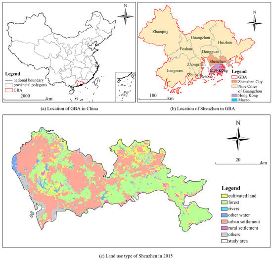
Figure 1.
Location of and land-use types in Shenzhen.
2.1.2. Dataset
The CDE raw data used in this study is the 10 × 10 km spatial resolution CDE data released by CHRED in 2015. This dataset integrates information on industrial energy consumption and processes, agriculture, services, urban lifestyles, rural lifestyles, and transportation emissions. According to information provided on the official website (http://www.cityghg.com, accessed on 15 July 2025), this dataset was constructed using a unified data source and standardized data processing methods to create a Chinese urban CDEs dataset [55,56]. Several prerequisites were followed when applying this dataset. First, based on existing research, the distribution of CDEs is directly influenced by human activities and exhibits significant positive spatial correlation. Second, the CDE data used in this study are annual averages and do not account for the severe short-term impacts on meteorological elements, particularly within the same city. Third, due to the mobility and diffusivity of CDEs and the neglect of wind and rainfall effects, there may theoretically be a phenomenon where CDEs decay with increasing distance from high-value regions to surrounding areas. In addition to CDE data, there are also auxiliary data (Table 1). The supplementary data include 2015 national population 1 km grid data, 2015 national nighttime light 1 km grid data, 2015 national land use 1 km grid data, and 2015 national NDVI vegetation index 1 km grid data. All these data are sourced from the China Resource and Environment Science and Data Center (RESDC, https://www.resdc.cn, accessed on 15 July 2025).

Table 1.
Data and their sources employed in this study.
2.2. Theoretical Framework
The spatial distribution of CDEs exhibits significant spatial heterogeneity, primarily driven by the spatial differentiation of human socio-economic activities [57]. As key indicators of urban systems, urban spatial structure, functional organization, and spatial layout all exert profound influences on the distribution patterns of CDEs. It is worth noting that cities, as highly open complex systems, engage in significant carbon exchange processes with surrounding regions, resulting in the boundaries of urban carbon cycles often extending beyond the spatial scope of central urban areas. Empirical studies have shown that there is a significant positive correlation between the level of urban economic development and the carbon influence range of its peripheral regions [58]. However, existing research on CDEs has two main limitations: on the one hand, the research scale is primarily focused on the macro and meso levels; on the other hand, it overlooks the spatial coupling relationship between CDEs and land use. The root cause of these research limitations lies in the method of obtaining carbon emission data: natural carbon flux data primarily comes from fixed-point observations, while socio-economic emission data is mostly based on statistical calculations at administrative unit levels (provincial, municipal, or county-level, with some studies reaching the township or street level), leading to difficulties in spatial matching between the two. Based on this, this study focuses on addressing the following two key scientific questions: (1) how to achieve high-precision spatial matching of CDEs within urban scales using CHRED; (2) how to utilize the high-resolution grid units and spatial differentiation characteristics of CDEI data to construct a spatial zoning framework for CDEs within cities using the “ring-layer and direction” method.
This study uses a three-step method to achieve spatial refinement analysis of urban carbon emission data (Figure 2). The specific process is as follows:
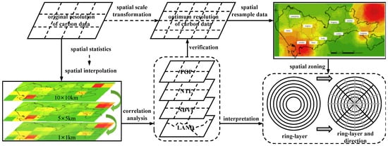
Figure 2.
Analytical framework of the study.
Step 1: Spatial downscaling of carbon emissions data. To address the issue of insufficient spatial resolution in the 10-km grid data of CHRED, this study employed spatial interpolation techniques to downscale the original city-level CDEs, effectively resolving the simulation issue of carbon emissions intensity decaying with distance, and achieving a scale conversion from low-resolution to high-resolution data [59].
Step 2: Determination of optimal spatial resolution. By systematically analyzing the spatial correlation between downscaled carbon emissions data and multi-source auxiliary data (including socioeconomic statistics, nighttime light remote sensing, and land use data) at different grid scales, a resolution optimization model was established to determine the optimal grid unit size for subsequent spatial zoning studies.
Step 3: Multi-scale spatial zoning of carbon emissions. Based on the selected resolution, multi-level ring-shaped analysis units are constructed. By quantitatively analyzing the variability characteristics of carbon emission intensity within and between rings, the spatial differentiation patterns of carbon emissions in Shenzhen are systematically revealed. This method achieves multi-level spatial pattern analysis of carbon emissions from macro-regional to micro-grid scales, providing a spatial analysis foundation for precise control of urban carbon emissions.
2.3. Methods
2.3.1. Grid Refinement
For studies of CDEs at the urban scale, the 10 × 10 km resolution grid is too coarse to capture surface detail features, making spatial interpolation techniques an effective means of converting the original 10 km grid CDE data into high-resolution units. The refinement of the original 10 km resolution data uses 1 km grid units as the basic unit. The CDEI values of the newly generated grid units are obtained by calculating the ratio of the total CDEI of the original 10-km grid units to their surface area, i.e., the CDEI value per square kilometer. Based on this, the center points of the newly generated 1-km grid units are extracted, and the CDEI values of each unit are assigned as the attribute values of the corresponding center points. Kriging interpolation is then performed to generate a spatial distribution map. This method is also applicable for generating spatial interpolation maps for 5-km and 10-km grid units.
2.3.2. Spatial Interpolation
Compared to a 10 km × 10 km grid, both the 5 km ×5 km grid and the 1 km × 1 km grid provide a more detailed representation of pollutant spatial distribution. However, from a spatial perspective, the distribution of pollutants exhibits poor transitional characteristics, with distribution curves that are highly irregular and inconsistent with the typical spatial distribution patterns of atmospheric pollutants in the air, as well as violating the first law of geography. Further processing is required.
Three methods—KRIGE (kriging), IDW (inverse distance weighting), and natural neighbor—were applied to perform spatial interpolation of CO2 data for the 5 km × 5 km grid. After interpolation, the average CO2 values for each 5 km grid were re-extracted and correlated with the original values, as shown in Table 2. The interpolation results from the IDW and natural neighbor methods exhibited the highest correlation with the original values.

Table 2.
Comparison of results obtained using different interpolation methods in this study.
2.3.3. Ring-Layer and Direction Analysis
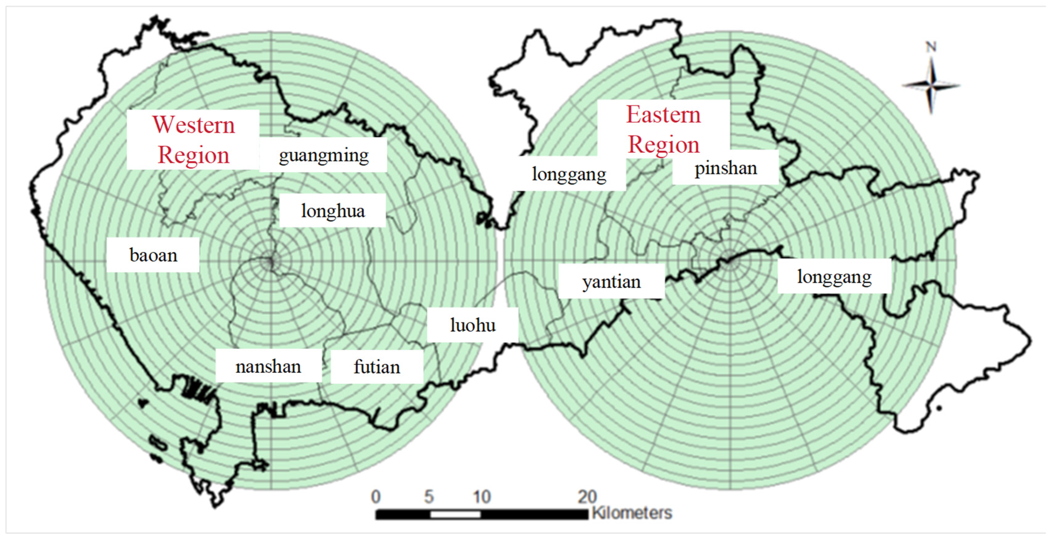
After determining the optimal resolution for data resampling, it is necessary to reveal the attenuation phenomenon of CDEs as the distance increases from high-value areas to surrounding areas. This study uses changes in CDEI values across different hierarchical levels as a metric, employing a circular hierarchical construction method. Taking the geometric center of the urban area as the reference point, circular hierarchical layers are constructed by expanding outward layer by layer to summarize the spatial distribution patterns of CDEs, thereby establishing the relationship between urban land use scale and pollutant emission intensity. Considering Shenzhen’s elongated east–west orientation and the lack of coastal carbon dioxide emission intensity data, two circular hierarchical groups were established in the eastern and western regions, respectively.
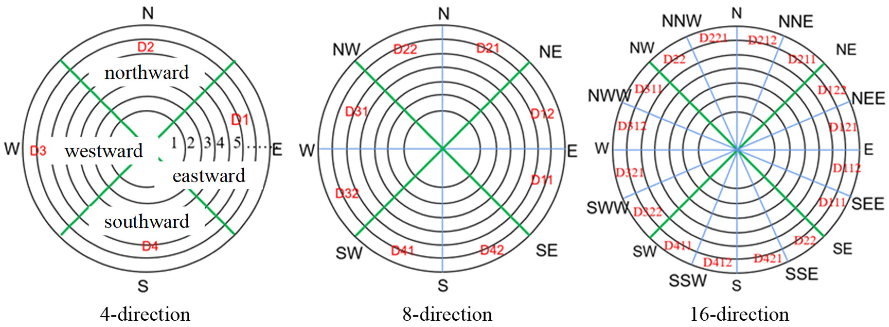
To further distinguish spatial differences in pollutant distribution across different directions, this study incorporates directional factors into the hierarchical framework for statistical analysis of pollutant emissions. As shown in Figure 3, the directional design includes 4-direction, 8-direction, and 16-direction configurations, where numbers such as 1, 2, and 3 represent hierarchical levels.
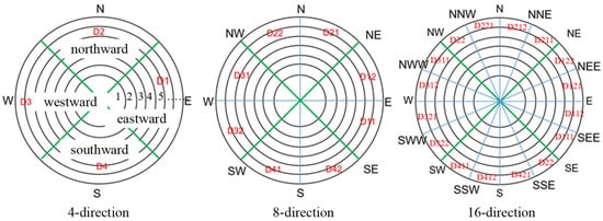
Figure 3.
Ring-layer and direction construction diagram.
When subdividing directions, as shown in Figure 3, the range extending 45° to either side from the true east direction is defined as the east direction D1. This direction is further subdivided into two sub-directions: east–southeast (D11) and east–northeast (D12). These directions are further subdivided into four smaller directions within the 16-direction grid: D111, D112, D121, and D122. Similarly, the range extending 45° to either side of true north is defined as the north direction D2, which is further subdivided into two sub-directions: northeast (D21) and northwest (D22). The range extending 45° on either side of true west is defined as the west direction D3, which is further subdivided into two sub-directions: northwest (D31) and southwest (D32); the range extending 45° on either side of true south is designated as the south direction D4, which is further subdivided into southwest (D41) and southeast (D42). The corresponding sub-directions are shown in Figure 3 (16-direction diagram).
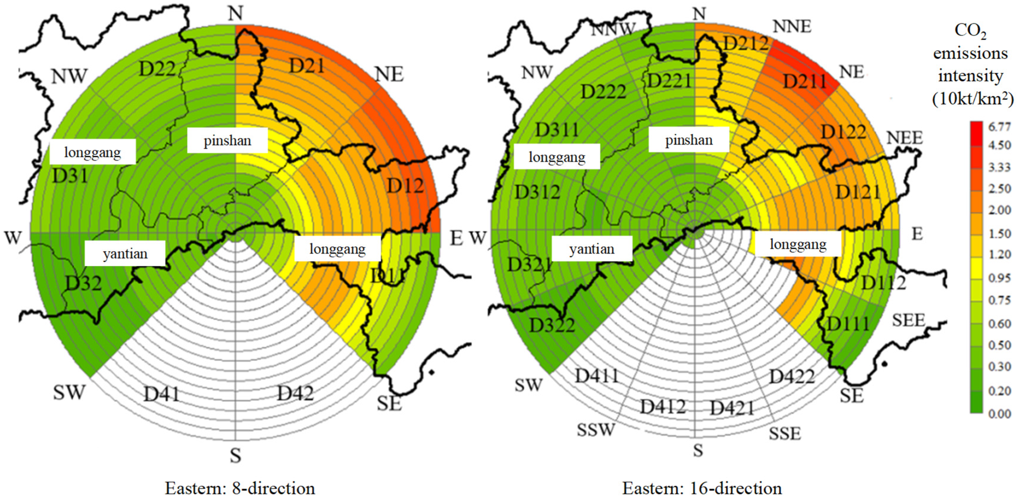
As shown in Figure 4, in the two concentric layers of Shenzhen, the western layer is centered at point (E113.962, N22.654), and the eastern layer is centered at point (E114.366, N22.641). Each layer expands outward in concentric circles, with each circle’s radius increasing by 1 km, forming a total of 21 concentric rings. The average carbon dioxide emission intensity for each independent layer is calculated.
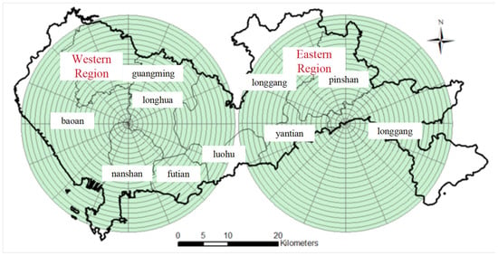
Figure 4.
Construction of Shenzhen’s “Ring-layer and Direction” model.
3. Results and Analysis
3.1. Spatial Analysis of CO2 in Shenzhen Based on Reconstructed Data
3.1.1. Overall Characteristics of CO2 Emission Intensity in Shenzhen
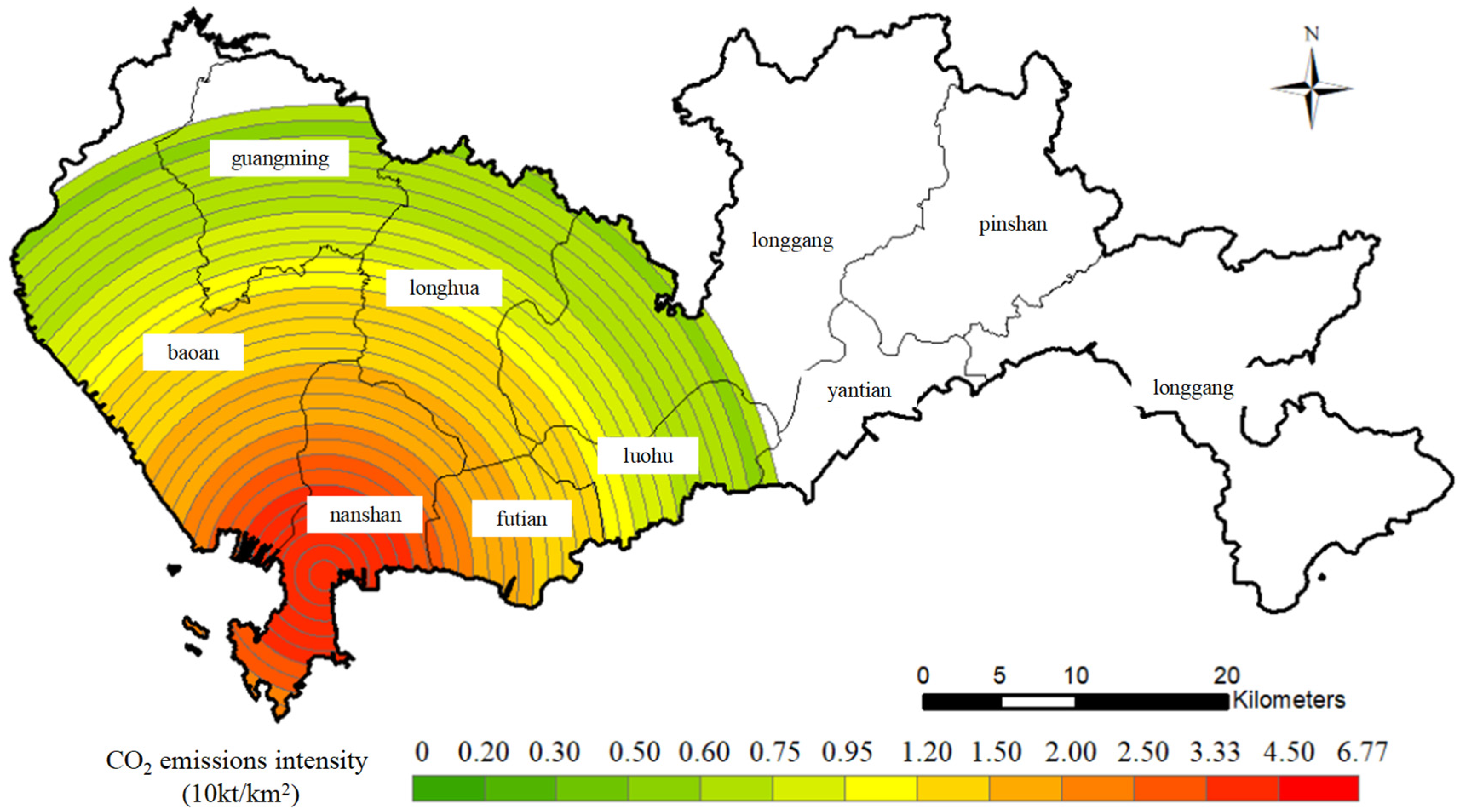
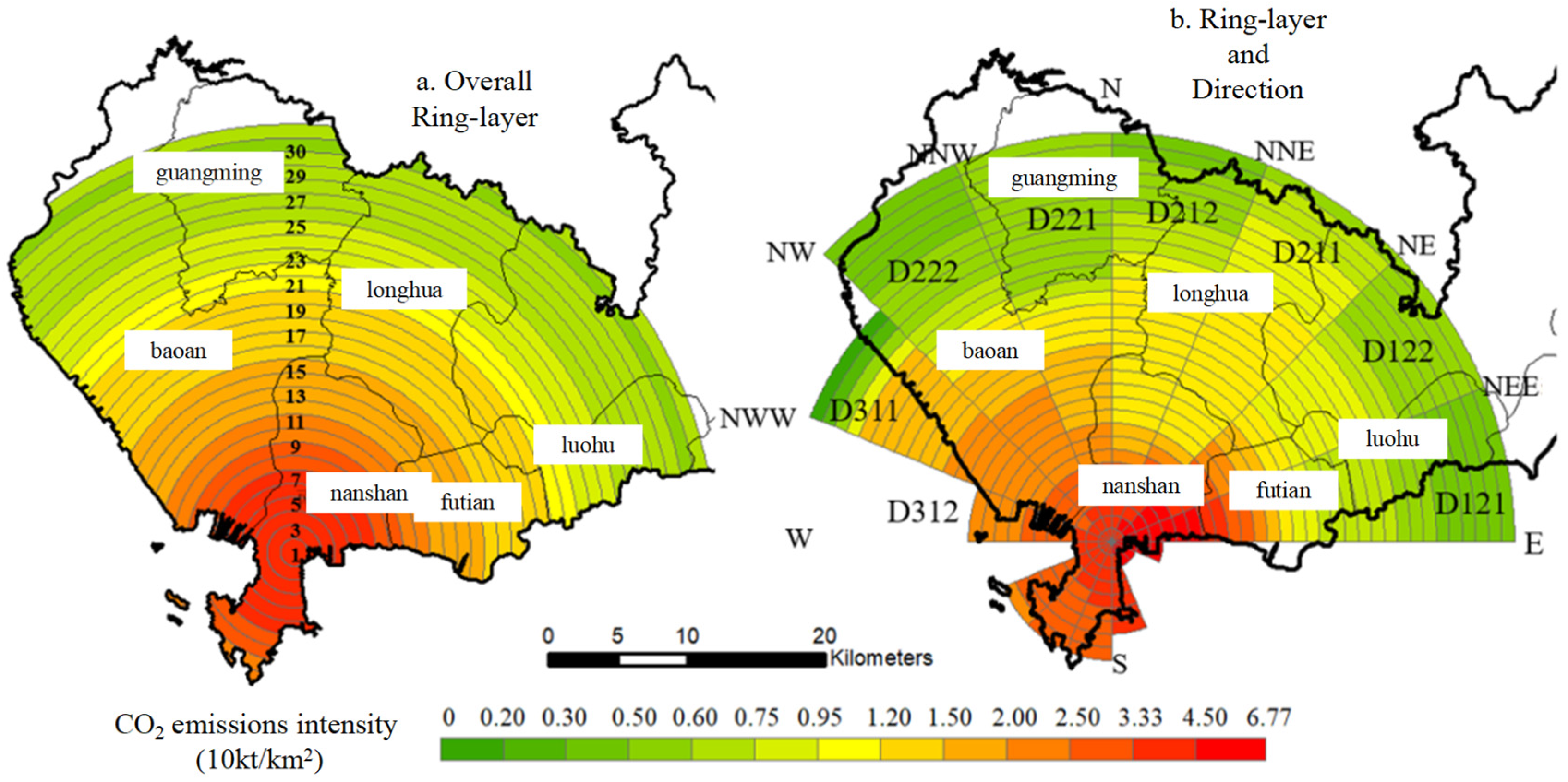
Considering the mobility and contagiousness of pollutants, the study selected the entire area shown in Figure 5, which contains a total of 4513 grid cells with a total area of 4513 km2. The area divided according to the grid centers located within the boundaries of Shenzhen contains a total of 2318 grid cells with an area of 2318 km2.
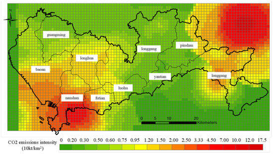
Figure 5.
Spatial distribution of CO2 emission intensity based on interpolation processing.
As shown in Table 3, within the city limits of Shenzhen, the city’s boundaries cover a total area of 2318 grids, equivalent to 2318 km2. Among these, 38 grids lack data. In the remaining 2280 km2, the average CO2 emission intensity is 1.00 kt/km2, with a maximum value of 6.77 kt/km2 and a minimum value of 0.10 kt/km2. When categorized by different CO2 emission levels, the area with low emission intensity is the largest, covering 1385 km2, accounting for 59.75% of the total. Within this category, the area in the 0.00~0.50 range is slightly larger than that in the 0.51~1.00 range, with only a small difference in area; the area with medium emission intensity is the second largest, covering 811 km2, accounting for 34.99% of the total; the area with high-intensity emissions (3~7 million tons/km2) is 84 km2, accounting for 3.62% of the total area; no ultra-high-intensity emission areas were identified within Shenzhen city limits.

Table 3.
Statistics on CO2 emission intensity within the scope of the study.
In summary, CO2 emissions within Shenzhen are mainly of medium to low intensity (<30,000 tons/km2), with low-intensity emissions accounting for approximately 60% and emissions below 20,000 tons/km2 accounting for as much as 87.19%.
3.1.2. Analysis of CO2 Distribution Characteristics in the Western Region of Shenzhen
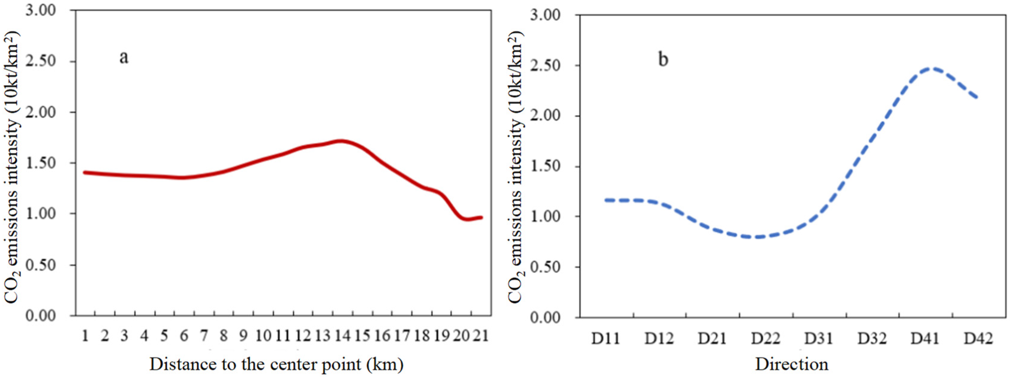
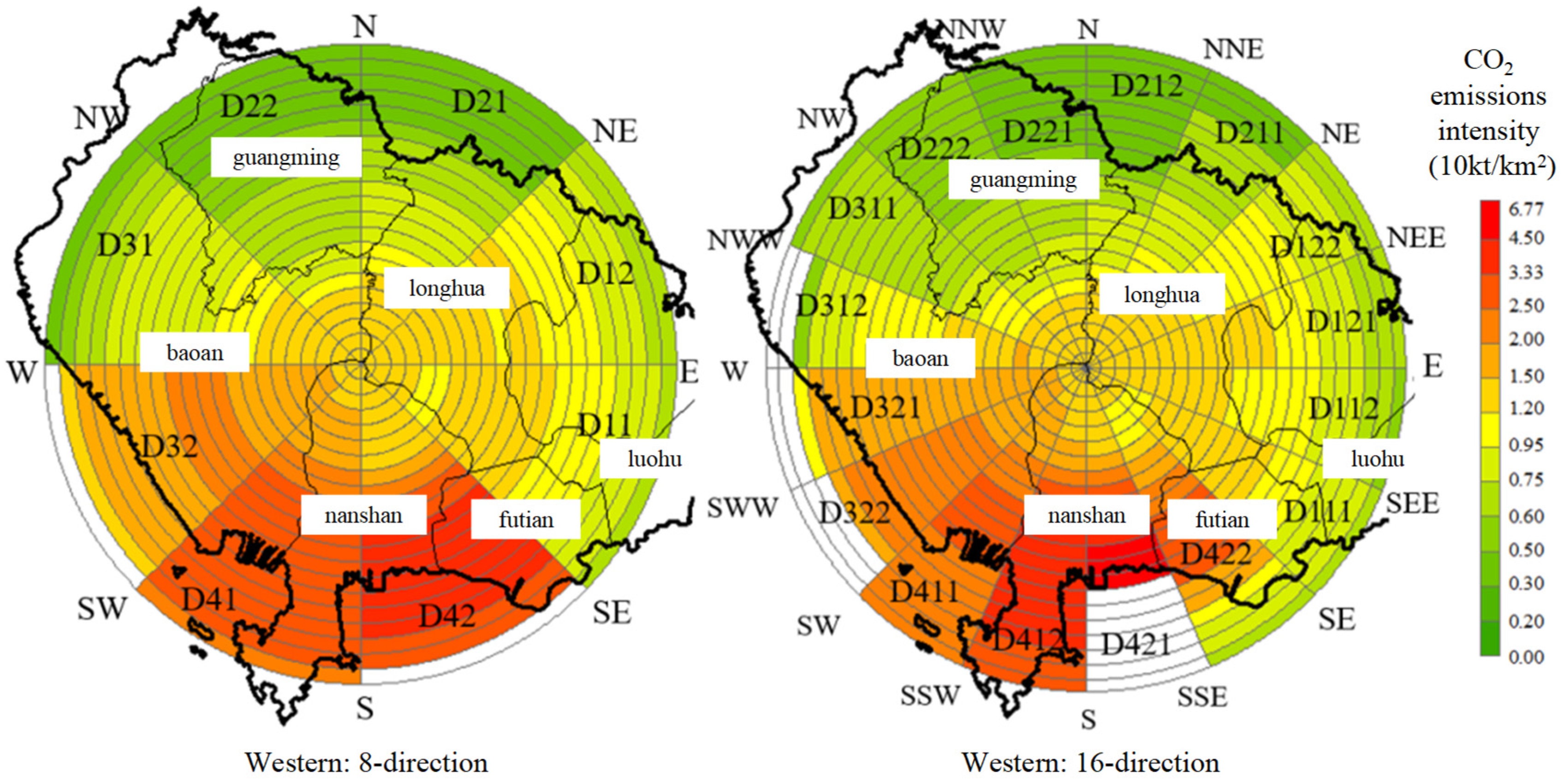
Figure 6 and Figure 7 illustrate the relationship between CO2 emission intensity and distance under the “ring-layer and direction” model in the western region of Shenzhen. From the perspective of ring-layer changes (Figure 6a), when the distance from the center (D) is between 0 and 8 km, the western region of Shenzhen is in a stable phase, with CO2 emission intensity ranging from 1.3 to 1.5 million tons per square kilometer, classified as moderate emission intensity; when the distance is between D = 9~14 km, CO2 emission intensity increases rapidly, reaching a peak when the distance is around D = 14 km; when the distance is greater than D > 15 km, CO2 emission intensity decreases rapidly, remaining at a low value and stable when D = 20 km. From the perspective of changes in different directions (Figure 6b), high values primarily appear in the southern directions D41 and D42 of the western region of Shenzhen, with smaller differences in other directions.
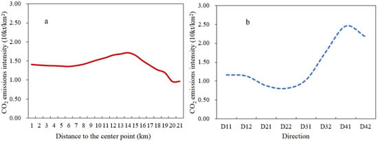
Figure 6.
CO2 distribution in the western part of Shenzhen (a) shows stratum changes; (b) shows differences between sub-directions.
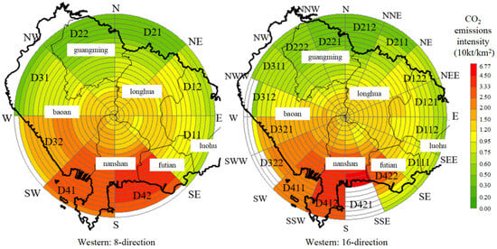
Figure 7.
CO2 distribution in the western region of Shenzhen under the “ring-layer and direction” model.
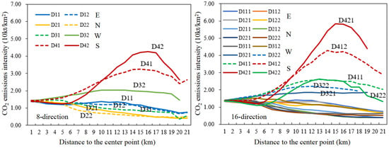
Figure 8.
Statistical distribution of CO2 in the western region of Shenzhen.
(1) Spatial variation of CO2 emissions in the eastward direction. The eastward direction refers to the D11 and D12 directions among the 8 directions (including the four sub-directions D111, D112, D121, and D122 among the 16 directions). The overall trend in the eastward direction shows a slight decrease in a stable manner.
From an average perspective, when the distance from the center is D = 0~5 km, the CO2 emission intensity ranges from 1.2 to 1.5 million tons per square kilometer, with relatively stable changes; when D = 5~10 km, there is a slight increase in stability; within the D = 10~16 km range, the smaller directions gradually reach their peaks; and when D = 16~21 km, the CO2 emission intensity remains stable with a slight decrease.
(2) Spatial differences in CO2 emissions in the northward direction. The northward direction refers to the D21 and D22 directions among the 8 directions (including the D211, D212, D221, and D222 sub-directions among the 16 directions). The overall trend in the northward direction is similar to that in the eastward direction, showing a slight decrease in a stable manner.
From an average state perspective, when the distance from the center is D = 0~5 km, CO2 emission intensity ranges from 1.2 to 1.5 million tons/km2, with relatively stable changes and a slight increase; within the D = 6~21 km range, CO2 emission intensity remains relatively stable with a slight decrease.
(3) Spatial differences in CO2 emissions in the westward direction. The westward direction refers to the D31 and D32 directions among the 8 directions (D311, D312, D321, and D322 among the 16 sub-directions). There are significant differences among the sub-directions in the westward direction.
The overall trend of the west–northwest direction D31 is similar to that of the north direction, showing a steady decrease. The overall average of the west–southwest direction D32 is higher than that of the east, north, and northwest directions. From the average change perspective, when the distance from the center is D = 0~5 km, the CO2 emission intensity ranges from 1.2 to 1.5 million tons/km2, with relatively stable changes and a slight increase; when D is between 6 and 10 km, CO2 emission intensity increases and remains stable at a high value of 2.0 to 2.5 million tons per square kilometer; when D is between 11 and 20 km, CO2 emission intensity begins to decrease but remains at a medium–high value of 1.5 to 2.0 million tons per square kilometer.
(4) Spatial differences in CO2 emissions in the southern direction. The southern direction refers to the D41 and D42 directions among the 8 directions (D411, D412, D421, and D422 among the 16 sub-directions). Among the four major directions, the southern direction has the highest average value, and the overall trend in the southern direction is inverted V-shaped.
From an average perspective, when the distance from the center is D = 0~5 km, the CO2 emission intensity ranges from 1.38 to 1.77 million tons per square kilometer, with relatively stable changes but a slight increase; within the D = 6~14 km range, the growth rate of CO2 emission intensity accelerates and remains at a high level (2.0~4.0 million tons per square kilometer); when D is between 14 and 18 km, the growth rate of CO2 emissions slows down, reaching a peak (4.0~4.5 million tons/km2); when D is between 18 and 21 km, CO2 emissions rapidly decrease to around 2.0 million tons/km2. Differences in smaller directions are evident, with D421 significantly higher than other directions, having the highest average, followed by D412. The peak values are primarily located between 14 and 18 km from the center in these two directions.
3.1.3. Analysis of CO2 Distribution Characteristics in the Eastern Region of Shenzhen
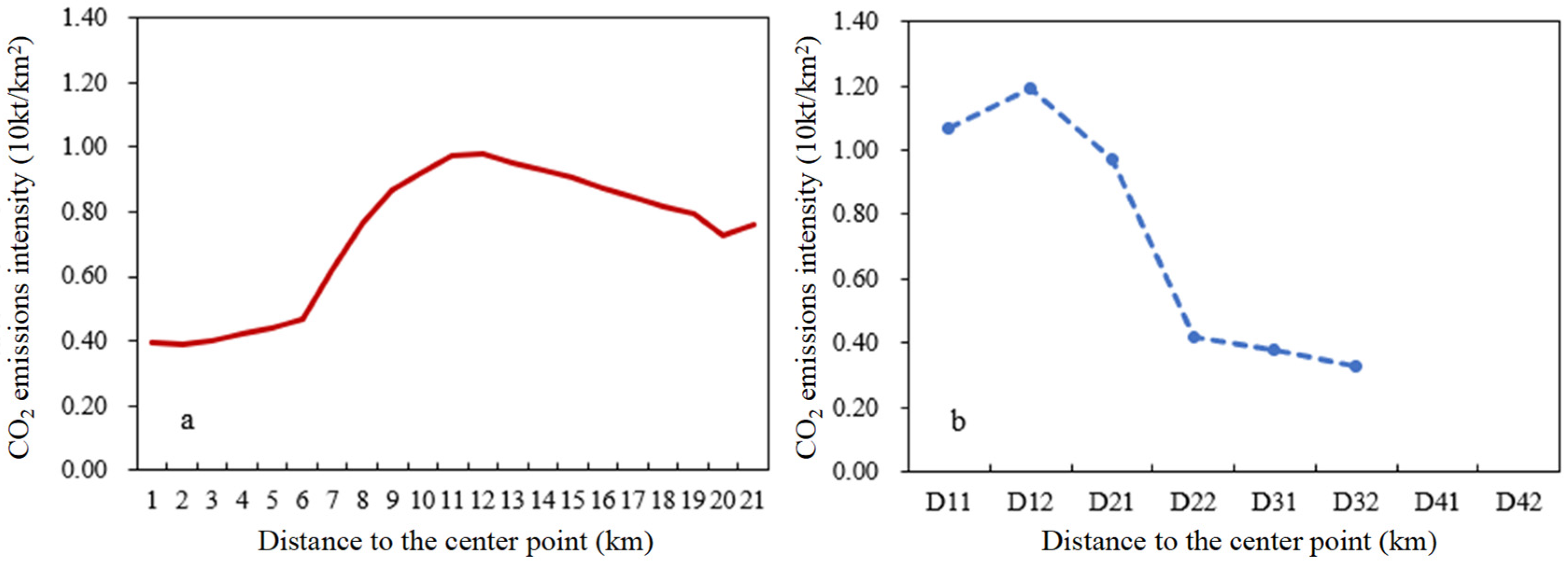
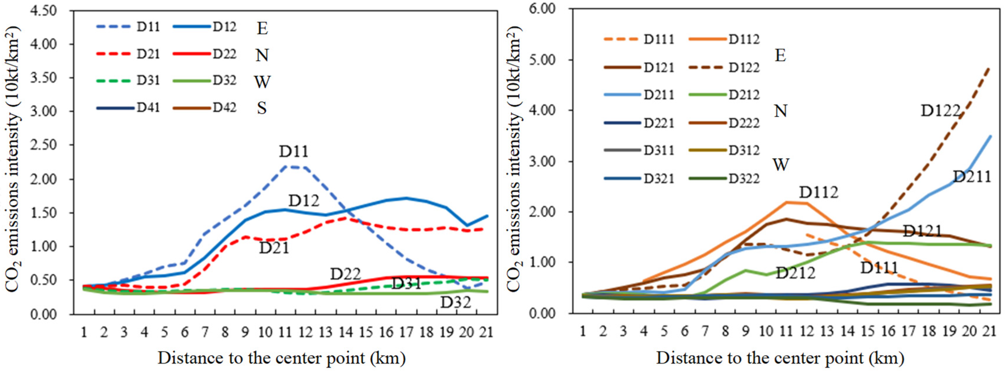
Figure 9 and Figure 10 illustrate the relationship between CO2 emission intensity and distance under the “ring-layer and direction” model in the eastern region of Shenzhen. From the perspective of layered changes (Figure 9a), in the eastern region of Shenzhen, when the distance from the center (D) is between 0 and 6 km, the CO2 emission intensity remains relatively stable with a slight increase, ranging from 0.3 to 0.5 million tons per square kilometer, indicating a relatively low emission intensity; when the distance is between 6 and 12 km (D = 6~12 km), CO2 emission intensity increases rapidly, reaching a peak of 0.98 million tons per square kilometer when the distance is around 12 km (D = 12 km); when the distance exceeds 12 km (D > 12 km), CO2 emission intensity decreases slowly, ranging from 0.70 to 0.98 million tons per square kilometer. From the perspective of changes in different directions (Figure 9b), relatively high values primarily appear in the eastward direction (D11 and D12) and northward direction (D21) of Shenzhen’s eastern region. The southward direction primarily lies outside Shenzhen, especially with missing data for D41 and D42. Differences in other directions are relatively small.
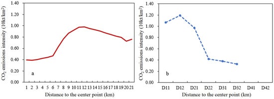
Figure 9.
CO2 distribution in the eastern part of Shenzhen (a) shows stratum changes; (b) shows differences between sub-directions).

Figure 10.
CO2 distribution in the eastern region of Shenzhen under the “ring-layer and direction” model.
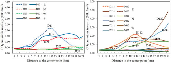
Figure 11.
Statistical distribution of CO2 in the eastern region of Shenzhen.
(1) Spatial differences in CO2 emissions in the eastward direction. The eastward direction refers to the D11 and D12 directions among the 8 directions (including the four sub—directions D111, D112, D121, and D122—among the 16 directions).
Overall, within the D = 1~6 km range, the CO2 emission intensity for both the D11 and D12 directions shows a slow increasing trend, maintaining relatively low values (between 0.5 and 0.8 million tons/km2); within the range of D = 6~21 km, there are significant differences. Specifically, the CO2 emission intensity of the eastward D11 direction accelerates, reaching a peak at D = 11~12 km, after which it begins to decline rapidly. A similar trend is observed in the sub-directions D111 and D112. Meanwhile, although the growth rate of D12 is relatively slow, it continues to increase until the outermost ring, particularly in the sub-direction D122, where the increase is rapid and significant. This is primarily influenced by the high-value area of Huishan in the northeast of Shenzhen.
(2) Spatial differences in CO2 emissions in the northward direction. This includes two directions (D21 and D22) among the 8 directions (and four sub-directions—D211, D212, D221, and D222—among the 16 directions).
The trends in D21 and D22 in the northward direction show significant differences. Among these, D21 exhibits a trend similar to that of the eastward direction, with CO2 emission intensity showing a slow increase within the D = 1~6 km range, maintaining relatively low values (between 0.5 and 0.8 million tons/km2); within the D = 6~21 km range, CO2 emission intensity continues to increase, particularly with rapid growth in the minor direction D211, and D212 also remains in a state of continuous increase. This area is similarly influenced by the high-value zone in the northeast of Shenzhen. The D22 direction within the northward direction exhibits a trend similar to that of the westward direction, maintaining low values (between 0.3 and 0.6 million tons/km2), which is also one of the lower-value zones across the entire Shenzhen region.
(3) Spatial differences in CO2 emissions in the westward direction. The westward direction refers to the D31 and D32 directions among the 8 directions (including the four sub-directions D311, D312, D321, and D322 among the 16 directions). The overall trend in the westward direction remains stable, maintaining low values (between 0.3 and 0.6 million tons per square kilometer), making it one of the lower-value zones across the entire Shenzhen region.
3.2. High Pollution Areas and Analysis of CO2 Absorption in the Surrounding Area
3.2.1. Construction of High-Value Zone Layers
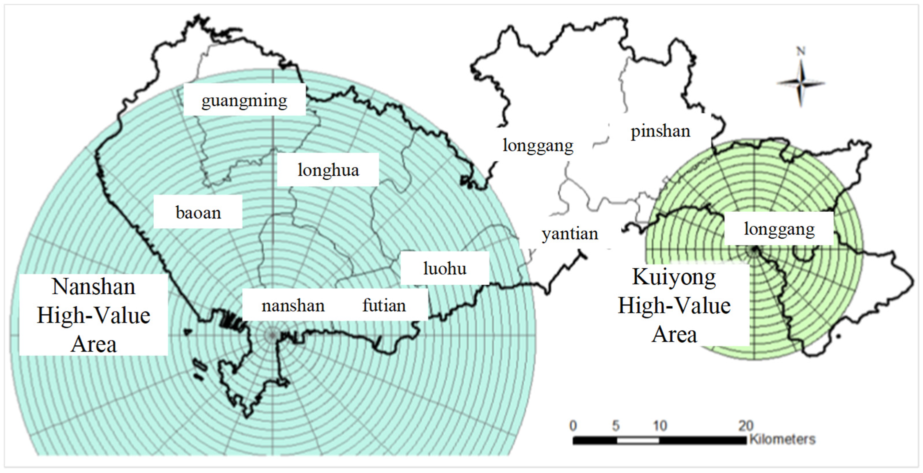
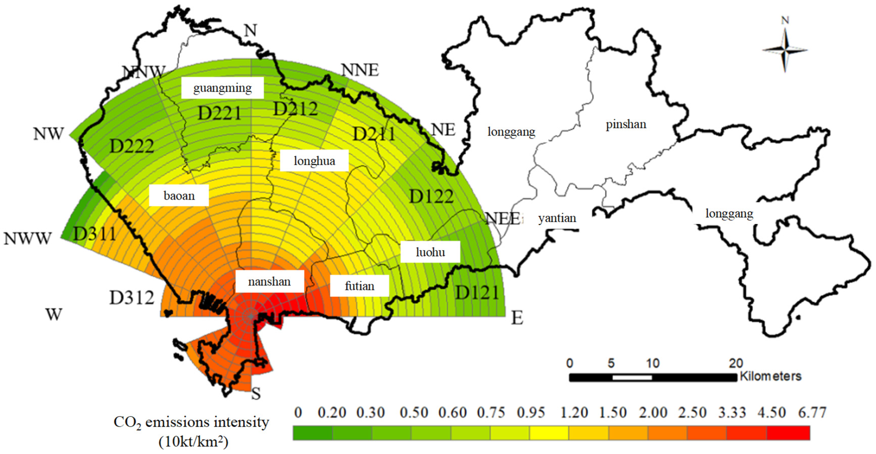
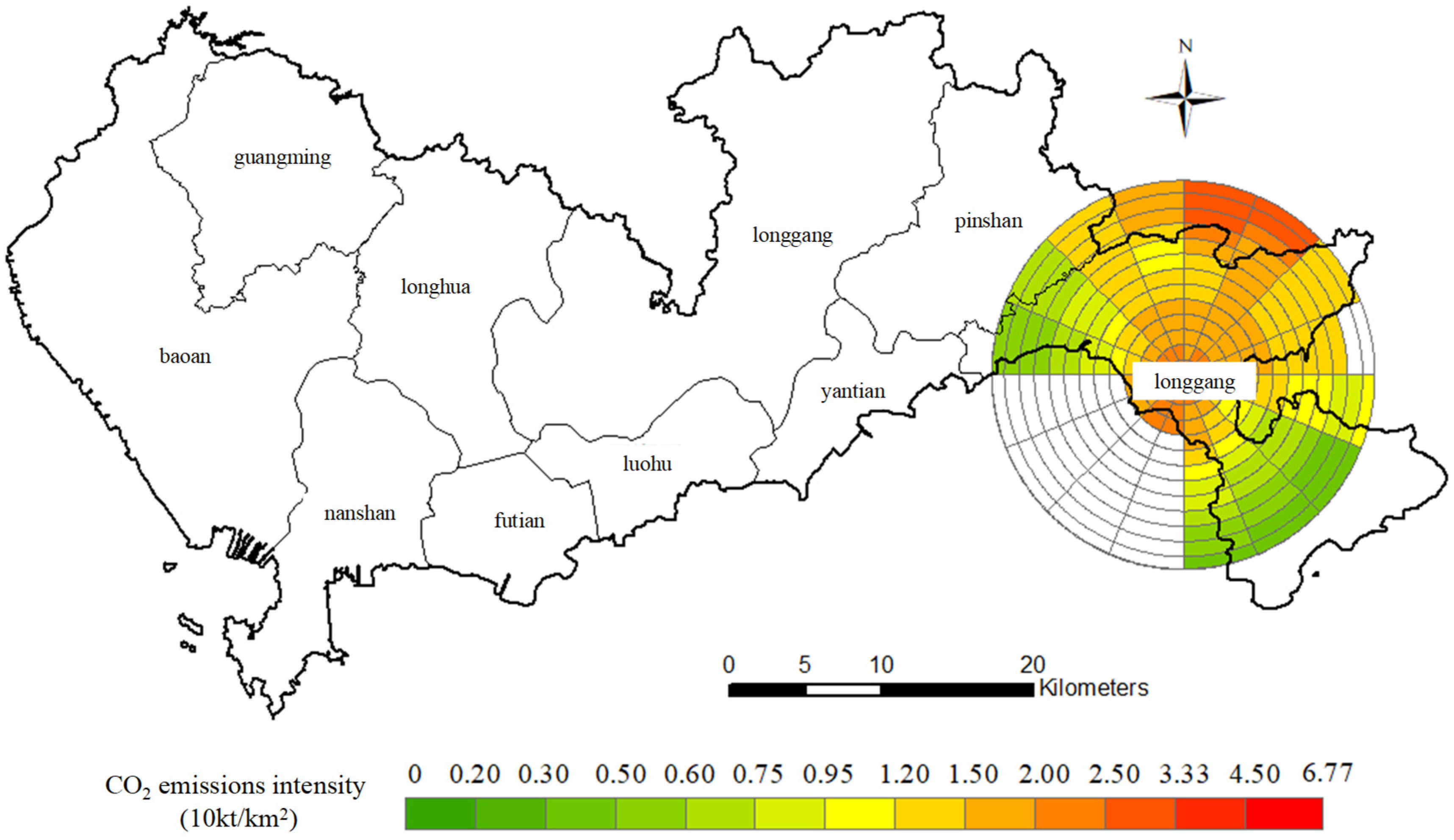
Shenzhen is elongated east–west and narrow north–south, with a complex urban boundary. Additionally, the city contains numerous mountainous areas, resulting in no distinct central concentration zone. From the perspective of CO2 emission intensity, two concentrated emission zones, or high-value zones, have emerged within Shenzhen: one along the coastline of the Nanshan region and the other in the Kuiyong Industrial Zone. In this section, we directly construct layers in these two high-value CO2 emission intensity zones, as shown in Figure 12. Each layer is centered on the high-value zone’s central point. The coordinates of the Nanshan high-value zone’s central point are (longitude 113.96, latitude 22.532), and those of the Kuiyong high-value zone are (longitude 114.443, latitude 22.56). The Nanshan high-value zone has 30 layers, while the Kuiyong high-value zone has 13 layers.
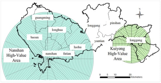
Figure 12.
Schematic diagram of the locations of high-value zones in Shenzhen.
3.2.2. Analysis of CO2 Changes in the Nanshan High-Value Area
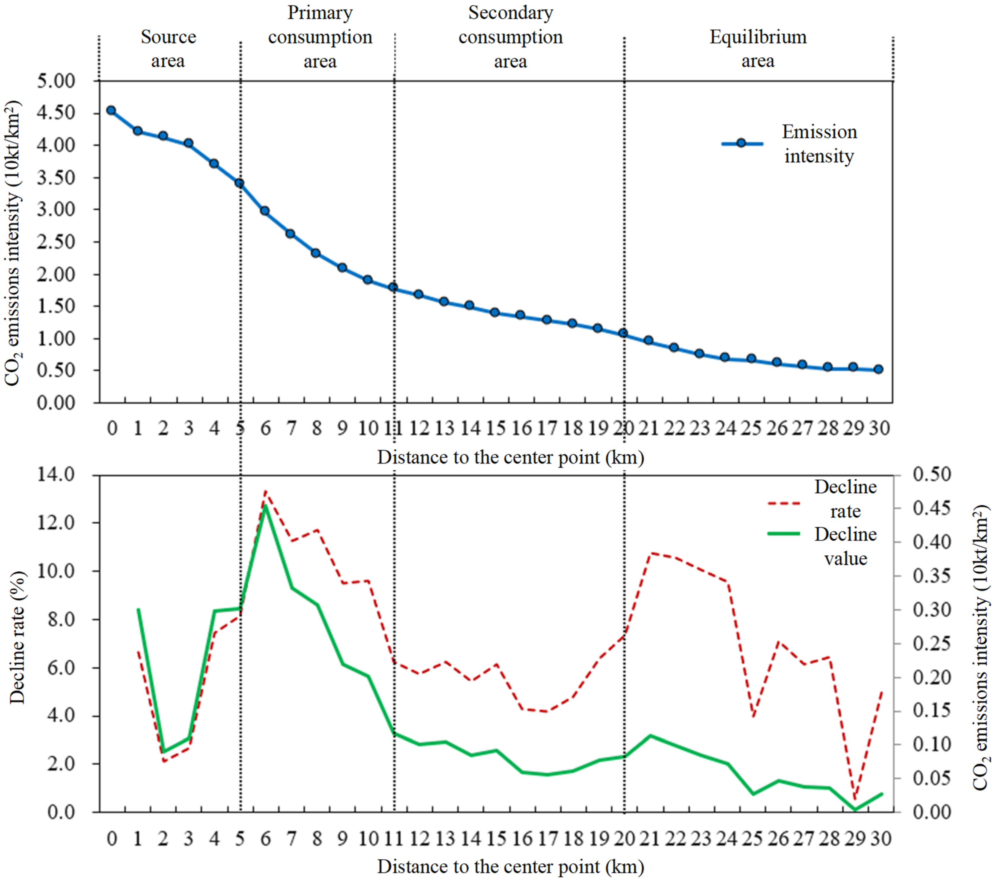
Figure 13 shows the changes in CO2 emission intensity in the high-value area of Nanshan. Among the 16 directions, only D121, D122, D221, D222, and D311 have valid data suitable for analysis. This section will only analyze these directions. Figure 14 shows the sequential decrease in CO2 emission intensity, i.e., the decrease in CO2 emission intensity of the nth layer compared to the (n − 1)th layer. The calculation formula is as follows: Δρ = (ρn − ρn − 1). Looking at the two figures together, it can be seen that the CO2 emission intensity of the high-value area in Nanshan decreases significantly from the center to the periphery of the circle. That is, as the distance increases, the CO2 emission intensity decreases first and then increases.

Figure 13.
CO2 concentration changes with stratification in the high-value area of Nanshan, Shenzhen.
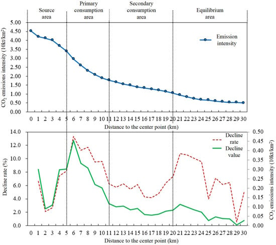
Figure 14.
Statistics on changes in CO2 emission intensity in the high-value zone of Nanshan.
The CO2 emission values in the first to fourth layers (0~5 km distance) are relatively high, exceeding 40,000 tons/km2, classified as high-intensity emission zones. Among these, the first layer has the highest average value at 45,100 tons/km2, while the second to fourth layers decrease sequentially to 40,100~42,100 tons/, with the decreasing values fluctuating layer by layer, indicating the source area; the CO2 emission values for the 5th to 11th layers range from 1.89 to 3.71 million tons per square kilometer, classified as moderate-intensity zones. As distance increases outward, the rate of CO2 reduction accelerates, with an average decrease of 9.65% per layer; layers 12~22 show a slower decrease in CO2 emission values, with average values per layer ranging from 0.94 to 1.78 million tons per square kilometer, and an average decrease of approximately 0.1 million tons per square kilometer per layer, indicating a reduced source effect; layers 23~30: CO2 emission values decrease to below 10,000 tons/km2, classified as a low-intensity zone, with an average layer-by-layer decrease of 0.05 million tons/km2, showing an overall stable trend.
After numerical quantification, the conclusions regarding pollutant emissions and absorption are as follows:
Let Q denote the ratio of the total pollutant absorption area to the source area, and let Q′ denote the ratio of the primary pollutant absorption area to the source area. Then, the absorption ratio of the Nanshan region under “high pollution conditions” is:
Q = STCA/SSA ≈ (400 + 200)/50 ≈ 12
Q′ = SPCA/SSA ≈ 200/50 ≈ 4
Let H denote the ratio of the total number of layers in the pollutant absorption zone to the source zone, and let H′ denote the ratio of the number of layers in the primary pollutant absorption zone to the source zone. Then, the absorption ratio of the Nanshan region under “high pollution conditions” is:
H = RCA/RSA = 20/5 ≈ 4
H′ = RPCA/RSA ≈ 6/5 = 1
Within the selected 30-km zone in the high-value area of Nanshan, the average CO2 concentration is 1.82 million tons per square kilometer, which is 1.82 times the average value for the entire city of Shenzhen (average CO2 emission intensity of 1.00 million tons per square kilometer). This is the highest value within the city of Shenzhen, with the maximum CO2 concentration within the selected zone reaching 4.51 million tons per square kilometer. The calculated primary absorption area is four times the size of the source area, with an additional one-fold expansion in spatial distance.
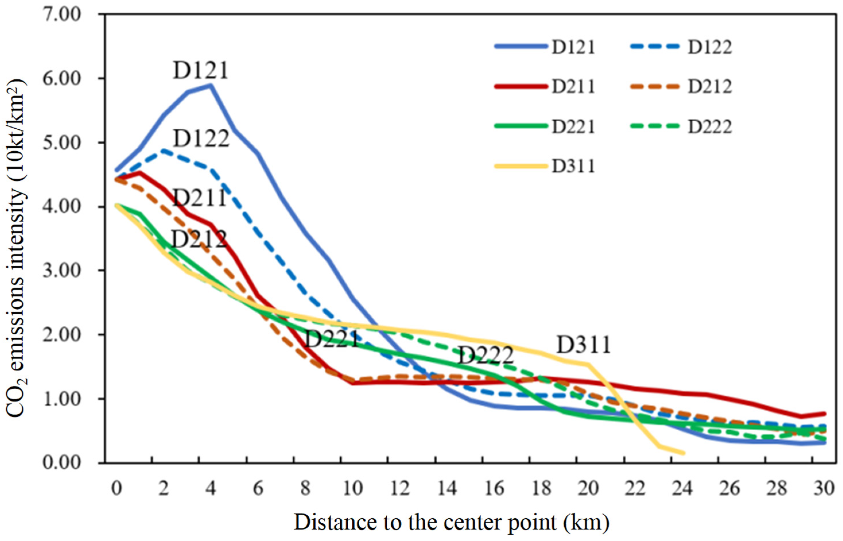
Figure 15 and Figure 16 illustrate the differences in CO2 variations across different directions within the Nanshan high-value zone. The results indicate that all sub-directions exhibit a decreasing trend, with specific differences lying in the varying degrees of reduction.
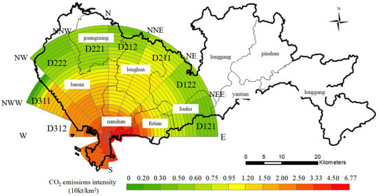
Figure 15.
Differences in CO2 concentrations in the high-value area of Nanshan, Shenzhen, depending on “ring-layer and direction”.
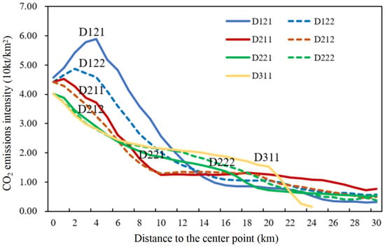
Figure 16.
CO2 concentration changes with stratification in the high-value area of Nanshan, Shenzhen.
(1) Eastward CO2 spatial variations. Here, “eastward” refers to the D12 direction among the 8 directions and the two sub-directions D121 and D122 among the 16 directions. From an average state perspective, when the distance from the center D = 0~4 km, the CO2 emission intensity ranges from 4.4 to 5.9 million tons per square kilometer, showing a slight increase; within the D = 4~5 km range, the two sub-directions gradually reach their peaks; within the D = 6~14 km range, CO2 emission intensity decreases rapidly; within the D = 15~30 km range, CO2 emission intensity remains relatively stable, with a slight decrease.
(2) Spatial differences in CO2 emissions in the northward direction. The northward direction refers to the D21 and D22 directions among the 8 directions, and the D211, D212, D221, and D222 directions among the 16 directions.
From the perspective of D21, when the distance from the center is D = 0~4 km, the CO2 emission intensity of D211 and D212 ranges from 3.5 to 4.5 million tons per square kilometer, maintaining a relatively high value with a slowing trend, though the deceleration is minimal; within the D = 5~11 km range, the CO2 emission intensity decreases rapidly; within the D = 12~30 km range, CO2 emission intensity decreases slightly but remains largely stable. From D22, when the distance from the center D is 0~4 km, the CO2 emission intensity of D221 and D222 ranges from 3.3 to 4.1 million tons per square kilometer, maintaining a high value with a gradual decrease and a significant deceleration; within the D = 5~11 km range, CO2 emission intensity decreases at an accelerated rate; within the range of D = 12~30 km, CO2 emission intensity continues to decrease, but the rate of decrease slows down.
(3) Spatial differences in CO2 emissions toward the west. In this section, “westward” refers to the D31 direction among the 8 directions and the two sub-directions D311 and D312 among the 16 directions. Due to limited data in the D312 direction, only D311 is analyzed.
When the distance from the center is D = 0~6 km, CO2 emission intensity ranges from 2.4 to 4.0 million tons/km2, with a relatively rapid decrease; within the D = 7~20 km range, the rate of decrease in CO2 emission intensity slows down, remaining relatively stable; within the D = 11~30 km range, most areas have entered marine regions, resulting in data gaps that cause the average value to drop sharply.
3.2.3. Analysis of CO2 Changes in the Kuiyong High-Value Area
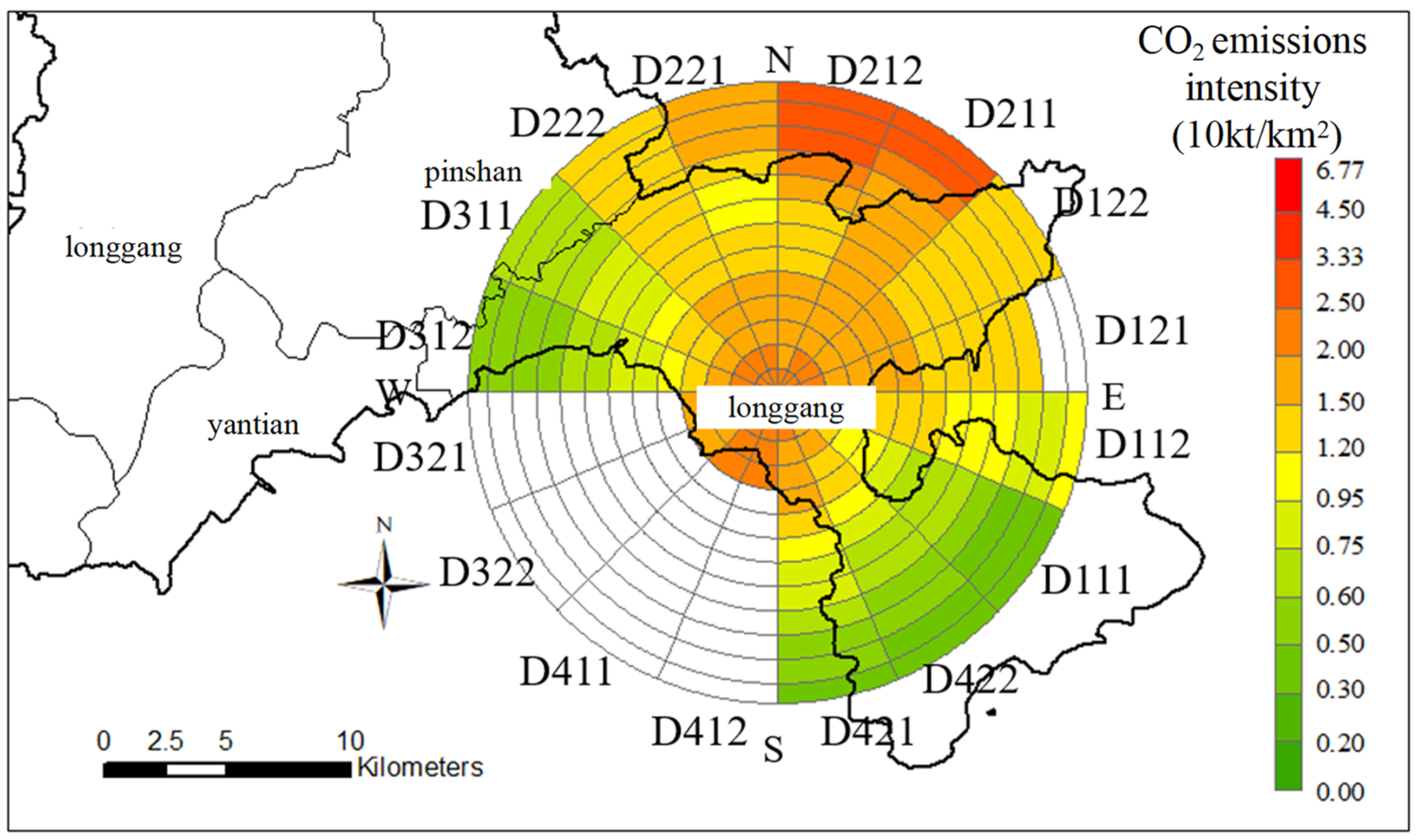
Figure 17 shows the layered schematic diagram of the Kuiyong Industrial Zone. Due to the absence of coastal data and the influence of the high-value zone in Huizhou to the northeast, the Kuiyong high-value zone is only divided into 13 layers. Figure 17 illustrates the changes in CO2 emission intensity of the Nanshan high-value zone. Data for D321, D322, D411, and D412 in the 16 directions are missing and are not included in the analysis.
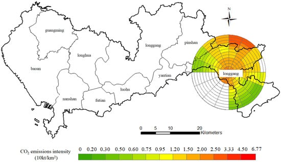
Figure 17.
CO2 changes in the high-value area of Kuiyong, Shenzhen.
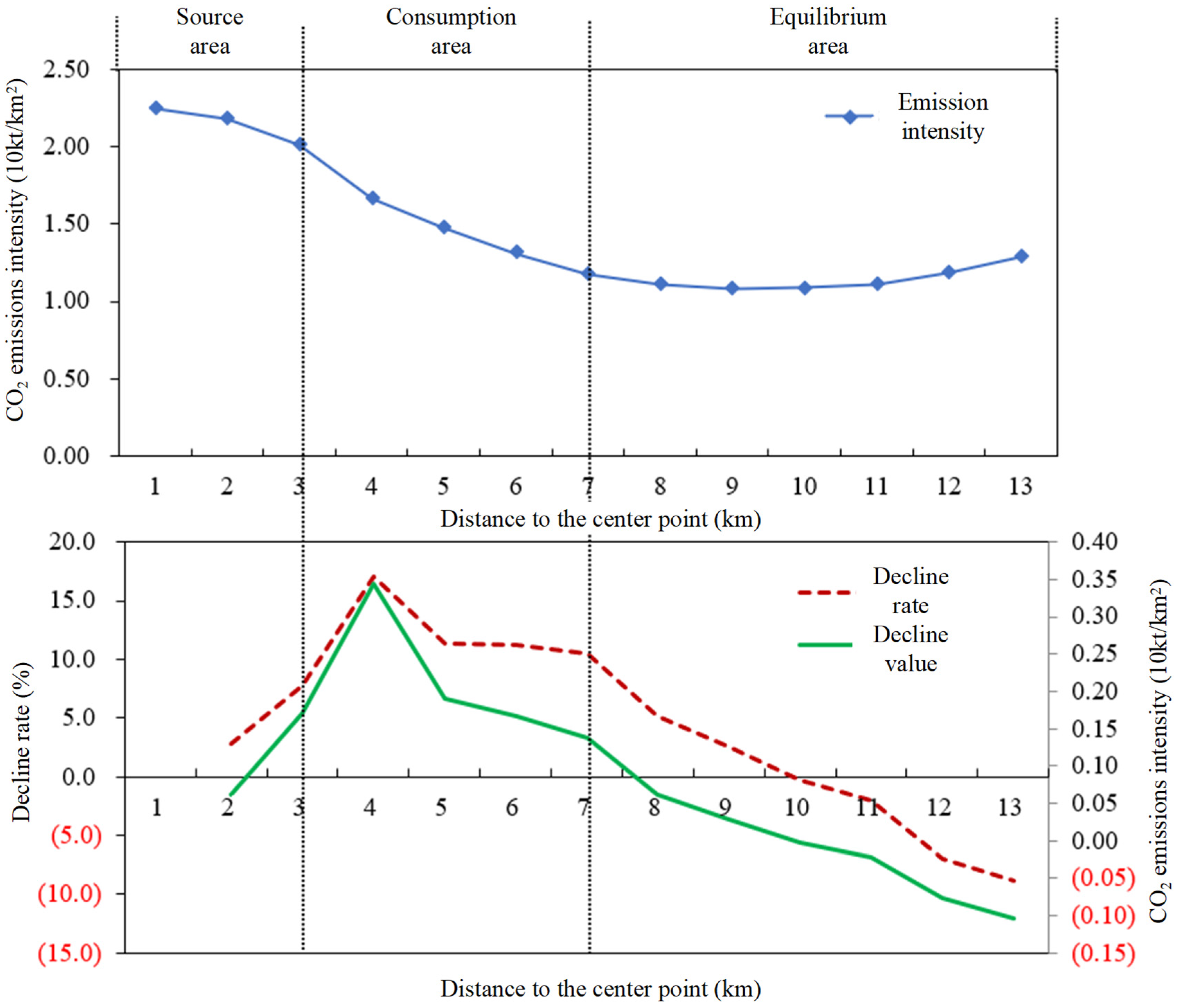
Figure 18 presents the statistical analysis of CO2 emission intensity in the Kuiyong high-value zone. The results indicate that the CO2 emission values in the first three zones (0~4 km) are relatively high, averaging around 20,000 tons/km2, representing a higher emission intensity within the region. Among these, the first zone has the highest value at 22,400 tons/km2, which is 1.54 times the average value within this range. The second and third layers decrease sequentially to 2.01 and 2.18 million tons per square kilometer, respectively, representing the source area. The average CO2 emissions for layers 3 to 7 are 1.62 million tons per square kilometer, classified as a moderate-intensity zone. As distance increases outward, CO2 emissions decrease at an average rate of 11.61% per layer. Layers 7~11 exhibit stable CO2 emissions, with an average decrease of approximately 0.04 million tons per square kilometer per layer; layers 11~13 show an increasing trend in CO2 emissions, primarily influenced by the high-value zone in northeastern Huizhou.
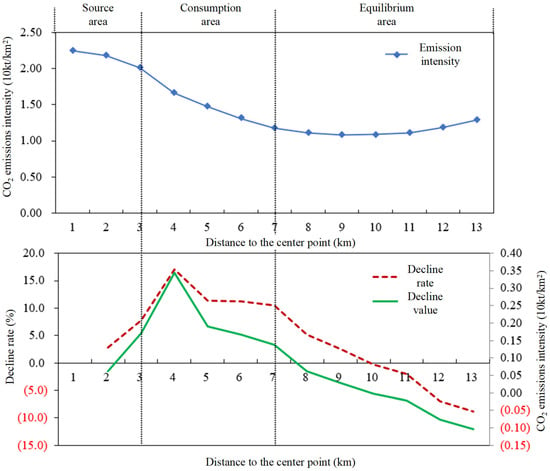
Figure 18.
Statistical analysis of changes in CO2 emission intensity in the high-value zone of Kuiyong.
After numerical quantification, the conclusions regarding pollutant emissions and absorption are as follows:
Let Q denote the ratio of the total pollutant absorption area to the source area; the absorption ratio of the high-value area in Kuiyong is as follows:
Q = SCA/SSA ≈ 130/30 ≈ 4
Let H denote the ratio of the total number of layers in the pollutant absorption zone to the source zone; the absorption ratio of the high-value area in Kuiyong is as follows:
H = RCA/RSA = 4/3 ≈ 1
Within the selected 13 zones in the high-value area of Kuiyong, the average CO2 concentration is 1.43 million tons per square kilometer, which is 1.43 times the average for all of Shenzhen (average CO2 emission intensity of 1.00 million tons per square kilometer). This makes it the second-highest value area after the Nanshan region. The highest CO2 concentration within the selected zones is 2.24 million tons per square kilometer. The calculated absorption area is four times the size of the source area, and the spatial expansion required is one times the distance outward.
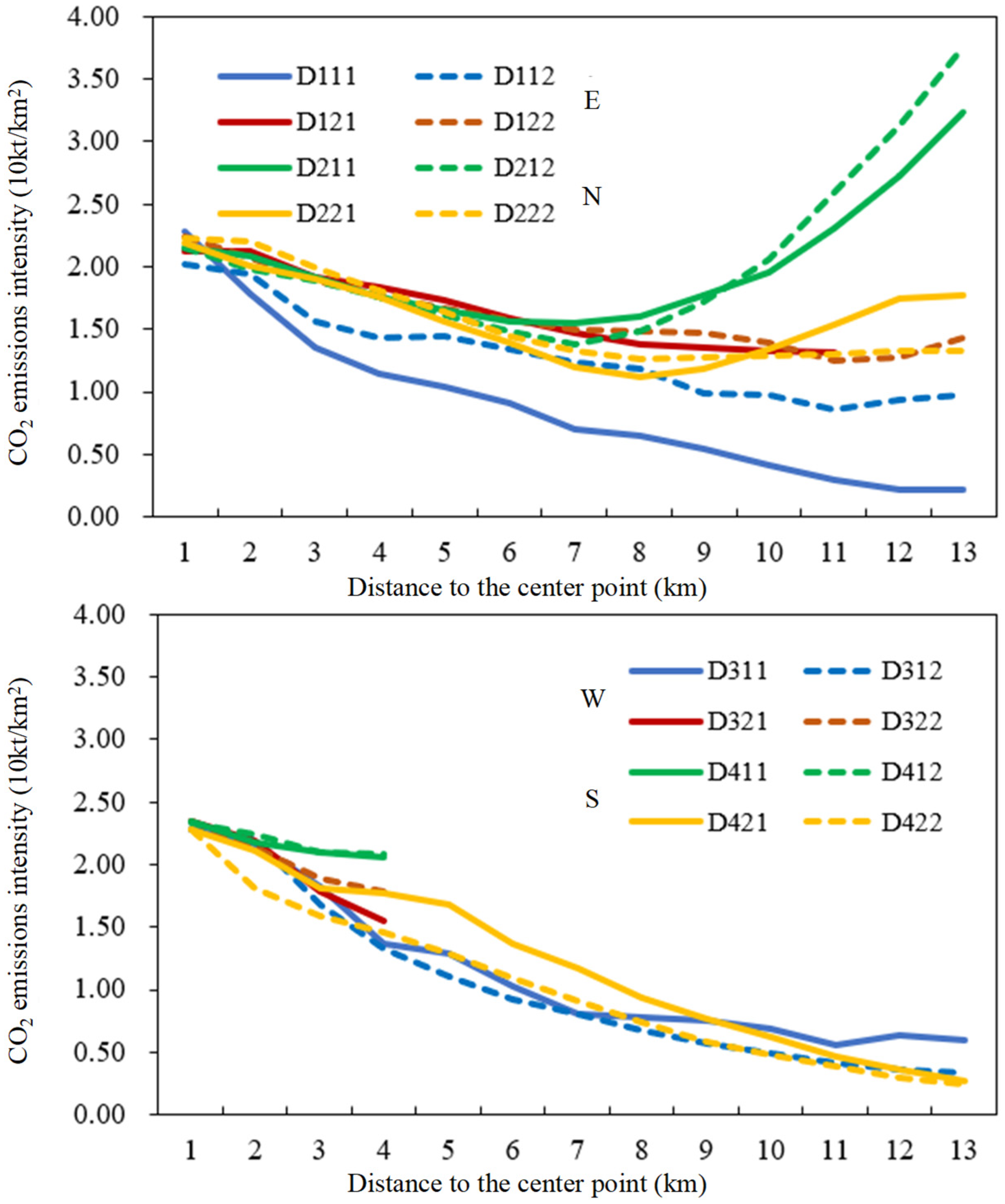
Figure 19 and Figure 20 illustrate the differences in CO2 attenuation across different directions within the high-value zone in Kuiyong. The results show that all sub-directions exhibit a decreasing trend, with the specific differences lying in the varying degrees of attenuation.
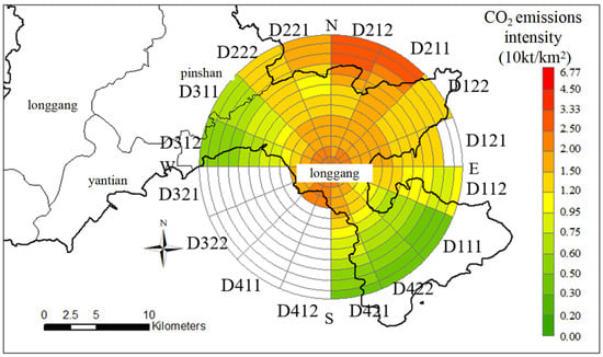
Figure 19.
Differences in CO2 concentrations in the high-value area of Kuiyong, Shenzhen, depending on “ring-layer and direction”.
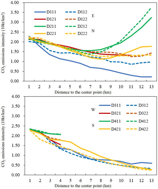
Figure 20.
CO2 concentration changes with stratification in the high-value area of Kuiyong, Shenzhen.
(1) Eastward. Here, eastward refers to the D11 and D12 directions among the 8 directions (D111, D112, D121, and D122 among the 16 directions) and the other four sub-directions. On average, when the distance from the center D = 0~2 km, the CO2 emission intensity of each direction is around 20,000 tons/km2, maintaining a high value but showing a decrease, which continues to decrease until the outermost layer. However, there are differences among the four directions. Within the range of D = 3~13 km, the CO2 emission intensity in the D111 and D112 directions continues to decrease but at a faster rate, while the decrease in the D121 and D122 directions is slower.
(2) Northward. The northward direction refers to the D21 and D22 directions among the 8 directions (and the D211, D212, D221, and D222 directions among the 16 directions). The CO2 emission intensity of the four sub-directions in the northbound direction is relatively high, and all exhibit a trend of first decreasing and then increasing. On average, when the distance from the center is D = 0~3 km, the CO2 emission intensity of all directions is around 20,000 tons/km2, maintaining a high value but with a slight decrease; within the range of D = 3~7 km, all four sub-directions show a stable decreasing trend, with the rate of decrease slightly increasing. Within the D = 7~13 km range, D221 remains stable, while the other three sub-directions show varying degrees of increase, primarily due to the significant influence of the high-value zone in Huizhou.
(3) Westward. Due to limited data, the westward direction here refers only to D31 among the 8 directions (D311 and D312 among the 16 directions). On average, when the distance from the center is D = 0~2 km, the CO2 emission intensity is around 20,000 tons/km2, maintaining a high value but slightly decreasing; in the range of D = 2~7 km, the decrease accelerates; within the D = 7~13 km range, both directions continue to decrease, but the rate of decrease slows.
(4) Southward. Due to limited data, the southward direction here refers only to D42 among the 8 directions (D421 and D422 among the 16 directions). These two directions show a generally continuous decreasing trend within the selected range, but the rate of decrease slows within the D = 9~13 km range.
3.3. Analysis of Factors Affecting CO2 Emission Intensity in Areas with High Pollution Levels
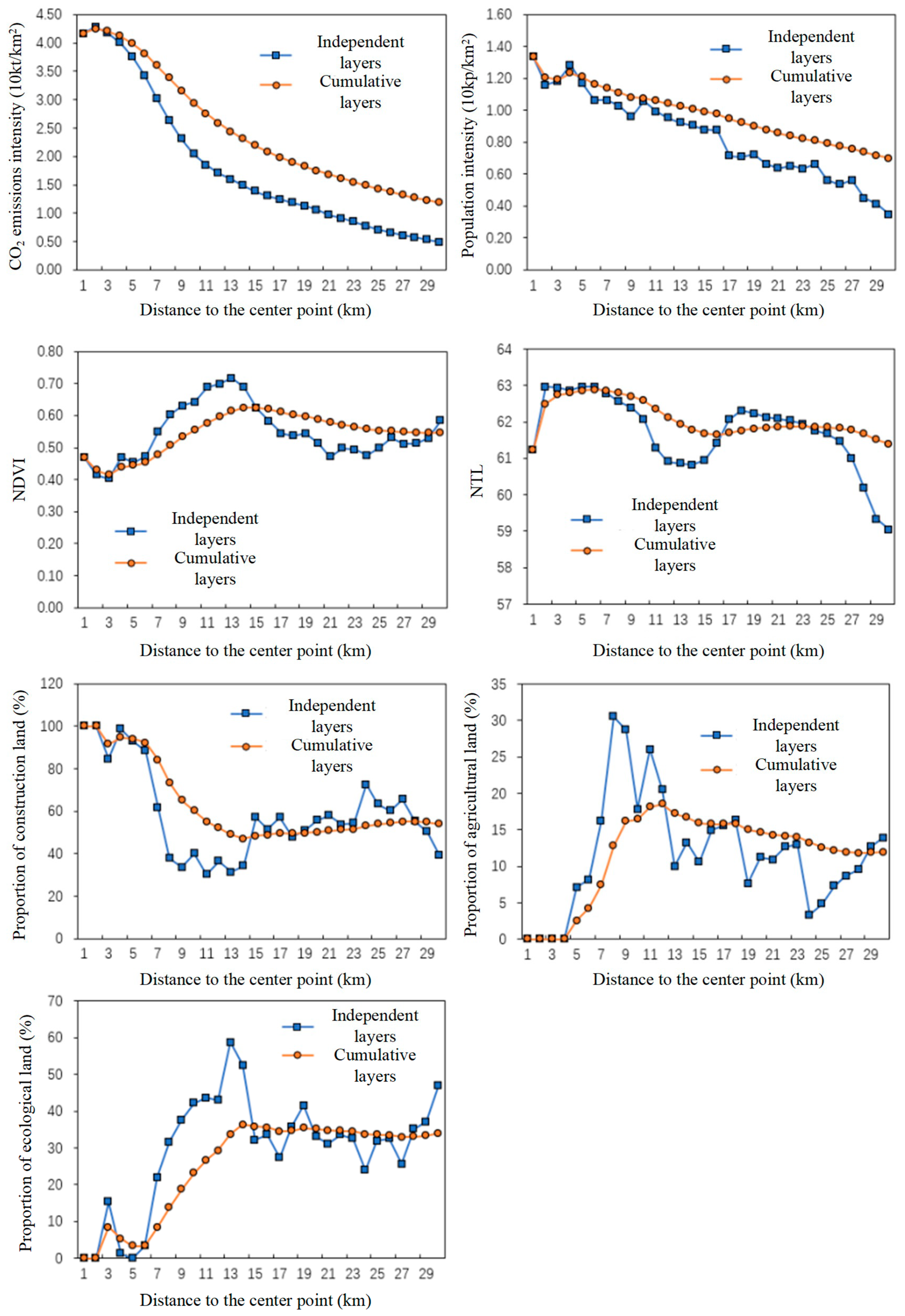
Based on the influence factor system in Table 4 and the zones in Figure 21, we analyzed the relationship between CO2 emission intensity and influence factors in the high-value area of the Nanshan region, Shenzhen. The analysis focused on the 30 zones in the overall zone and each direction (D121, D122, D211, D212, D221, D222), and was conducted from two aspects: independent zones and cumulative zones.

Table 4.
Construction of the impact factor system.
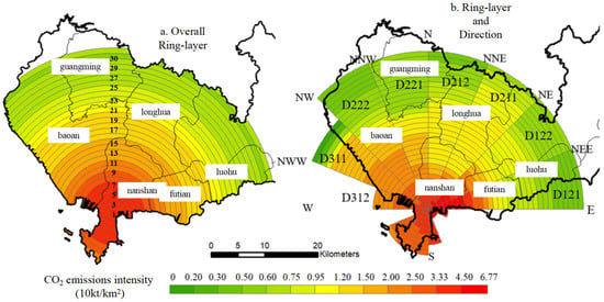
Figure 21.
CO2 changes in the high-value area of Nanshan, Shenzhen.
Figure 22 shows the statistical analysis of the changes in each influencing factor (including population density, light index, vegetation index, ratio of construction land area, ratio of agricultural land area, and ratio of ecological land area) across different zones. From the perspective of the 30-zone changes, both the independent zones and cumulative zones show a clear trend of decreasing CO2 emission intensity from the center outward (including the transition from coastal to inland areas in the Nanshan region).
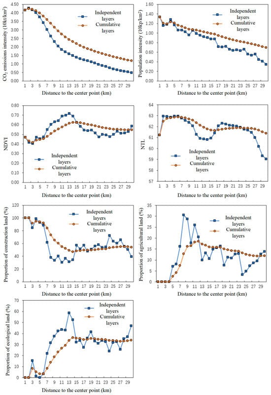
Figure 22.
Circular changes in influencing factors.
The corresponding situations for each influencing factor are as follows:
(1) Population density distribution. Independent concentric layers show that the average population density fluctuates and decreases from the center to the periphery, but the overall downward trend is relatively obvious, decreasing from 13,400 people/km2 in the central layer to 4100 people/km2 in the outermost layer, with an average decrease of 4.25%. In the cumulative zones, this curve is smoother, with the average population density decreasing across all 30 zones to 0.72 thousand people per square kilometer as the zones expand outward. The correlation coefficients R between population density and CO2 emission intensity are 0.992 (independent zones, p < 0.01) and 0.970 (cumulative zones, p < 0.01), respectively, indicating a significant positive correlation between CO2 emission intensity and population density. Linear regression indicates that an increase of one unit in population density leads to an increase of 4~5 units in CO2 emissions.
(2) Light index. The independent layer shows that the average light index fluctuates from the center to the outer layers, exhibiting an inverted “W” trend. The average light index across all layers is 61.71. When D = 0~10 km, the average light index values across all layers range from 61.22 to 62.78, with little variation; at D = 11~14 km, the light index drops to 60.88, maintaining a relatively low value; subsequently, at D = 15~26 km, the light index rises again to around 62.0; at D = 27~30 km, it drops below 61. The overall trend across independent layers is downward, with an average decrease of 0.12%. In the cumulative layer, this curve becomes more stable, with an overall change rate of −0.01%. As the layer expands outward, the light index changes from 61.22 in the first layer to 61.39 across all 30 layers. The correlation coefficients R between the light index and CO2 emission intensity are 0.613 (independent layer, p < 0.01) and 0.720 (cumulative layer, p < 0.01), respectively, indicating a significant positive correlation between CO2 emission intensity and population density. Areas with higher light indices have greater CO2 emission intensities. Linear regression analysis indicates that an increase of one unit in the light index leads to an increase of 0.75~1.53 units in CO2 emissions.
(3) Vegetation index. The independent layer shows that the vegetation index in the layers exhibits a “first rising then declining” trend from the center to the periphery, resembling an inverted V-shape, but the overall trend is upward, with an average increase rate of 1.0%. The average vegetation index across all layers is 0.54. When D = 0~6 km, the vegetation index remains stable, fluctuating between 0.40 and 0.47; at D = 7~20 km, the vegetation index first increases from 0.55 to a peak of 0.72 (at D = 13 km), then gradually decreases back to 0.55, but remains above the average value; at D = 21~30 km, the vegetation index of the layer remains around 0.5 with minimal variation. In the cumulative stratum, the inverted V-shaped curve flattens out. When the stratum range is D = 14 km, the vegetation index within the statistical range reaches its maximum value of 0.62. Excluding the cumulative average vegetation index of approximately 0.45 within the D = 7 km range, the vegetation index generally ranges between 0.55 and 0.62 as the range expands. The correlation coefficients R between the vegetation index and CO2 emission intensity are −0.312 (independent layer, p = 0.09) and −0.754 (cumulative layer, p < 0.01), respectively. This indicates that there is no significant relationship between CO2 emission intensity and population density in the independent layer, but there is a significant positive correlation in the cumulative layer, suggesting that as the layer expands outward, the larger the overall vegetation index, the lower the CO2 value. Linear regression indicates that for every unit increase in the vegetation index, CO2 emissions decrease by 12 units.
(4) Construction land. In the independent layer, the ratio of construction land area shows a trend of “first decreasing then stabilizing and fluctuating” from the center to the periphery, with an overall decreasing trend, averaging a decrease of 2.10 units. The average ratio of construction land area across all layers is 58.78%, with the highest value at the layer center, reaching 100%. Between D = 0~6 km, the ratio of construction land area remains at a high value, fluctuating between 88.42% and 100%; between D = 7~14 km, the ratio of construction land area decreases to approximately 34%; at D = 15~30 km, the average ratio of construction land area rebounds to around 56%, but remains far below the circle center. At this point, values across all circles range from 51.05% to 72.63%, with slightly greater fluctuations. In cumulative circles, the downward trend is significant, but the curve becomes flatter. As the circle area expands, the ratio of construction land area gradually decreases from over 90% at the center to around 50%. The correlation coefficients R between the vegetation index and CO2 emission intensity are 0.637 (independent zones, p < 0.01) and 0.885 (cumulative zones, p < 0.01), respectively, indicating a significant positive correlation between CO2 emission intensity and the ratio of construction land area, i.e., the higher the ratio of construction land area, the higher the CO2 value. Linear regression analysis indicates that an increase of one unit in the ratio of construction land area leads to an increase of approximately 0.05 units in CO2 emissions.
(5) Agricultural land. Changes in the independent layer show that the ratio of agricultural land area exhibits a trend of “first increasing then decreasing” from the center to the periphery, with significant fluctuations, but an overall increasing trend, averaging an increase of 0.48 units. The average ratio of agricultural land area across all zones is 11.65%. No agricultural land was recorded in the central zone (D = 0~4 km). Between D = 5~9 km, the ratio of agricultural land area rapidly increases from 7.14% to a peak of 30.57%. Between D = 10~30 km, it begins to fluctuate downward, with an average of 12.35% and slightly greater fluctuations. In the cumulative zones, the ratio of farmland area exhibits an inverted V-shape, with the peak shifted to the left. However, it still shows a clear trend of first increasing and then stabilizing as the zone area expands. The correlation coefficients R between the proportion of agricultural land area and CO2 emission intensity are −0.257 (independent zones, p = 0.17) and −0.689 (cumulative zones, p < 0.01), respectively. This indicates that there is no significant correlation between CO2 emission intensity and the proportion of agricultural land area in independent zones, but cumulative zones show a significant negative correlation between the two, meaning that the larger the proportion of agricultural land area, the lower the CO2 value. Linear regression analysis indicates that an increase of one unit in the ratio of agricultural land area leads to a decrease of approximately 0.12 units in CO2 emissions.
(6) Ecological land. Changes in the independent layer show that the ratio of ecological land area exhibits a trend of “initial increase followed by stable change” from the center to the periphery, with an overall increasing trend, averaging an increase of 1.62 units. The average ecological land area ratio across all layers is 29.49%. In the central layer (D = 0~6 km), ecological land is extremely low, with only the third layer showing 15% ecological land, while other layers are essentially 0%. Between D = 7~14 km, the agricultural land area ratio rapidly increases from 3.43% to a peak of 58.67%; it begins to decline at D = 15~30 km, especially within the range of D = 16~28 km, where it remains relatively stable, with an average of 32.45%. In the cumulative zones, the trend of the ecological land area ratio “first increasing then stabilizing” is particularly pronounced. As the zone area expands, the ecological land area ratio gradually increases from 0 to 36.25% within the D = 13 km range, after which it remains relatively stable. The correlation coefficients R between the ecological land area ratio and CO2 emission intensity are −0.729 (independent zones, p < 0.01) and −0.930 (cumulative zones, p < 0.01), respectively. Both indicate a significant negative correlation between CO2 emission intensity and the ratio of agricultural land area in independent zones, meaning that the larger the ecological land area ratio, the lower the CO2 value. Linear regression analysis indicates that an increase of one unit in the ecological land area ratio results in a reduction of approximately 0.06~0.08 units in CO2 emissions.
Overall, both population density and light intensity indices indicate the degree of urban development, with higher values indicating greater development. This is primarily because higher population density requires a relatively larger area of land for construction to accommodate the population, and the light intensity index, which reflects human activity, also increases accordingly. The two indices exhibit a certain degree of overlap and collinearity, and their effects on CO2 emissions are also relatively consistent, exhibiting an amplifying effect—that is, higher values correlate with greater CO2 intensity. The vegetation index reflects the extent of vegetation coverage on the ground surface. This not only refers to forested areas but also includes urban parks, grasslands, farmland, water bodies, wetlands, and other areas with varying degrees of vegetation coverage. Therefore, the vegetation index can comprehensively reflect the impact of urban greening on CO2. The results indicate that the higher the vegetation index, the stronger its role in absorbing CO2.
Among land use types, construction land has an exacerbating effect on CO2, primarily because construction land is a major source of CO2 emissions (from industrial and residential activities), and this source effect is widely accepted and recognized. Agricultural land exhibits seasonal variation patterns. During the growing season, vegetation has lush foliage and high coverage, thereby absorbing CO2. However, during the harvest season, vegetation coverage significantly decreases, and the use of mechanized equipment also leads to increased CO2 emissions. Therefore, agricultural land exhibits both source and sink effects on CO2; thus, this land use type is analyzed separately. However, based on the data analysis results, for the entire city, agricultural land has a stronger CO2 sink effect. Ecological land includes land use types such as forest land, grassland, and water bodies. However, according to Shenzhen’s current land use status, forest land accounts for a larger proportion, while grassland and water bodies have relatively smaller areas. The primary role of ecological land is primarily reflected through forest land.
4. Discussion
As a frontier of China’s reform and opening-up and a special economic zone, Shenzhen’s carbon emissions structure differs significantly from that of traditional industrial cities. Although Shenzhen’s industrial system is dominated by high-tech industries, sectors such as electronics manufacturing, advanced equipment manufacturing, new energy, and biopharmaceuticals remain the primary sources of its carbon emissions. Among these, the electronics manufacturing sector has a high energy intensity, particularly in chip manufacturing and display panel production, where its carbon emissions intensity and scale are significant. Additionally, Shenzhen’s port logistics, transportation, and construction sectors are also significant sources of carbon emissions [60]. It is worth noting that Shenzhen’s energy structure is relatively diverse, and in recent years, it has actively promoted renewable and clean energy sources, such as distributed photovoltaics and hydrogen energy, to reduce reliance on traditional fossil fuels. According to Shenzhen’s 14th Five-Year Plan, by 2025, the added value of green and low-carbon industries is expected to reach CNY 200 billion, and the city plans to establish 100 pilot projects for near-zero carbon emission zones to drive the low-carbon transformation of industries [61]. However, Shenzhen still faces the challenge of balancing industrial upgrading with carbon emission control, especially in the context of global supply chain fluctuations and changing market demands. Ensuring the economic viability of low-carbon technology investments has become a key challenge.
Shenzhen’s urban spatial development exhibits typical high-density, intensive characteristics, and its functional zone CDEI may be relatively low due to compact urban planning. Similar to Nanjing, Shenzhen’s mixed land use model and public transportation priority strategies (such as subway networks and bus lanes) help reduce commuting carbon emissions [52]. Additionally, Shenzhen has distinctive ecological space planning, such as the “Shenzhen Mountain-Sea Vistas” [62] initiative to strengthen the urban green space system, enhance carbon sink capacity, and improve climate resilience through sponge city construction. However, Shenzhen’s urban expansion still faces land resource constraints, and development in emerging areas (such as the Shenzhen–Shanwei Special Cooperation Zone) must be cautious of the carbon emission growth risks associated with low-density sprawl. Research indicates that optimizing urban spatial layout, such as promoting TOD (Transit-Oriented Development) models [63] and integrated planning of industry, residential areas, and ecology [64], can effectively reduce overall carbon emission intensity.
As one of the core engines of the Guangdong–Hong Kong–Macao Greater Bay Area, Shenzhen’s low-carbon development is not only about local emissions reduction, but also serves as a model for regional carbon reduction cooperation. Shenzhen has taken the lead in exploring carbon market innovations, such as promoting a “dual control” mechanism for carbon emission intensity and total volume, and plans to achieve dual control quota allocation for manufacturing carbon emissions by 2028 [60]. Additionally, Shenzhen is actively developing carbon finance, promoting carbon asset pledge financing, carbon bonds, and other products, and exploring marine carbon sink trading to promote emissions reduction through market-based measures [65]. In terms of regional collaboration, Shenzhen can strengthen cooperation with cities like Hong Kong and Guangzhou in the hydrogen energy industry chain, jointly establish Greater Bay Area hydrogen energy standards, and promote cross-border carbon market connectivity [66]. Meanwhile, leveraging the “Guangdong Carbon Label Information Management Platform” [67], Shenzhen can further strengthen product carbon footprint management, promote green supply chain development, and support low-carbon trade in the Greater Bay Area.
The national spatial planning system recently implemented by the Chinese government serves as the core policy framework for national land use and spatial development. By establishing a five-level planning implementation mechanism linking the national, provincial, municipal, county, and township levels, it systematically achieves the scientific identification and precise control of ecological protection, agricultural production, and urban development spaces [68]. This planning system provides systematic solutions for regional sustainable development by optimizing the spatial development and protection pattern, regulating land use structure, and improving spatial configuration efficiency. In the context of addressing climate change, this planning system demonstrates significant carbon emission reduction potential. Specifically, at the urban planning level, the following aspects should be prioritized: first, establish an economic development linkage model between county-level scales and urban CDEs to analyze the spatial development characteristics of different urbanization stages; second, formulate differentiated low-carbon development pathways and establish a spatial planning evaluation system incorporating core indicators such as total carbon emissions, CDEI, and carbon sink capacity; finally, quantitative indicators should be converted into operational spatial element allocation schemes to form a low-carbon spatial planning paradigm with regional adaptability. It is worth noting that international best practices indicate that carbon trading mechanisms and ecological compensation policies have achieved significant results in spatial planning. Research on the localization of these innovative policy tools in China will provide important theoretical support and practical references for the low-carbon transformation of national spatial planning [69,70]. By systematically integrating spatial planning with carbon emissions control systems, it is possible to achieve synergistic optimization between economic development and carbon reduction targets, ultimately fostering the formation of a high-quality development model characterized by green and low-carbon practices.
5. Conclusions
This study uses Shenzhen as a case example to address the technical challenges of obtaining micro-scale carbon emission data by employing spatial interpolation techniques to downscale 10-km grid carbon emission data, while systematically determining the optimal spatial resolution for carbon emission zoning through multi-source auxiliary data analysis, including socioeconomic statistics, nighttime light remote sensing, and land-use data. To reveal the spatial differentiation patterns of CO2 emission intensity in Shenzhen, the study constructs multi-level ring-shaped analysis units and examines directional differences across the region. Furthermore, the emission and absorption characteristics of high-pollution zones, such as the Nanshan region and the Kuiyong Industrial Zone, are analyzed to provide deeper insights into localized carbon dynamics. The key contributions of this study are as follows: (1) this study integrates CHRED with high-resolution remote sensing data, achieving high-precision spatial matching of carbon emission data and providing a scientific basis for precise carbon management at the urban scale; (2) the proposed “ring-layer and direction” analytical method addresses the limitations of traditional research in analyzing intra-city spatial differentiation of carbon emissions, particularly in examining directional variations; (3) the findings offer valuable insights for formulating low-carbon urban planning policies in Shenzhen and other high-density cities, such as optimizing land-use structures, adjusting industrial layouts, and enhancing ecological space protection.
This study finds that population density, nighttime light index, and construction land ratio showed strong positive correlations with CO2 emission intensity (R = 0.992, 0.720, and 0.885, respectively), and are the main drivers of carbon emissions in Shenzhen. And, vegetation index and ecological land ratio were negatively correlated with emission intensity (R = −0.754 and −0.930), underscoring the importance of ecological conservation in mitigating emissions. Overall, CO2 emissions in Shenzhen are primarily of low to medium intensity (<30,000 tons/km2), with low-intensity areas accounting for 59.75% and medium-intensity areas for 34.99%. High-intensity emission zones (3~7 million tons/km2) cover only 3.62% of the city. Significant spatial heterogeneity was observed, with the Nanshan region and the Kuiyong Industrial Zone identified as the two major high-emission zones, reaching peak intensities of 4.51 and 2.24 million tons/km2, respectively. Specifically, in the western region (centered on the Nanshan region), CO2 emission intensity remained stable (1.3~1.5 million tons/km2) within 8 km of the center, peaked at approximately 14 km, and then declined rapidly. In the eastern region (centered on Kuiyong), emission intensity was relatively low (0.3~0.5 million tons/km2) within 6 km of the center, peaked at 12 km, and then decreased gradually. In addition, directional differences were notable. For example, high values in Nanshan were concentrated in the southern directions (D41, D42), while Kuiyong’s emissions were significantly influenced by high-value zones in Huizhou to the northeast.
In the future, the growth rate of carbon emissions will continue to significantly exceed the rate of carbon sequestration, necessitating a larger external ecosystem to achieve balance. Clearly, as urban carbon source areas continue to expand, the CDEI of emerging areas, urban peak areas, and suburban decline areas will also continue to rise. At the same time, their coverage will continue to expand, causing existing external balance areas to gradually shrink. Industrial transformation is a viable solution to this issue. The emerging information and communications technology (ICT) industry holds potential for reducing carbon emissions [71], so megacities like Shenzhen must make strategic decisions regarding the development path of the ICT industry. Additionally, Shenzhen should further integrate multi-source high-resolution data to deepen the refined analysis of carbon emission driving mechanisms, particularly conducting industry-energy-land use coupling studies in key areas such as Nanshan and Kuiyong to quantify the synergistic benefits of industrial transformation and ecological restoration. Simultaneously, it is recommended to establish a “spatial heterogeneity-policy response” assessment framework to optimize the low-carbon layout model of “multi-center-networked” high-density cities through scenario simulation.
Evidently, the limitations of this study should be mentioned and need to be addressed in future studies.
(1) When studying carbon sources and sinks in terrestrial ecosystems, the limitations caused by scale effects are particularly significant. This study uses Shenzhen as a closed area for research and fails to fully consider the carbon exchange and carbon migration between Shenzhen and the larger surrounding areas (such as other cities in the GBA). This limits the comprehensive understanding of the overall pattern of regional carbon cycles and restricts the spatial extrapolation of the research conclusions to a certain extent.
(2) The resampled data for the spatial zoning division were derived from the 10 km spatial resolution of CHRED, and this study has refined the resolution problem by spatial interpolation in order to achieve spatial scale transformation. Therefore, the resampled data can only reveal the spatial heterogeneity characteristics of Shenzhen’s CDEs from the overall spatial pattern; they cannot accurately match the grid cells in the same locations. Moreover, despite its advantages, CHRED still suffers from gaps in coastal areas, potentially affecting the completeness of the analysis.
(3) With the development of urbanization and industrialization in Shenzhen, CDEs are still undergoing dynamic changes. Due to limitations in data collection and matching, this paper only obtained basic data from 2015, making it impossible to conduct empirical analysis of the annual changes in CDEI spatial zoning. This also limits the continuity and timeliness of the research conclusions in terms of time.
(4) Future research could further expand the application of the “ring layer and direction” analysis method in urban agglomerations such as the GBA, improving accuracy through multidimensional data verification to support the formulation of regional coordinated emission reduction policies.
Author Contributions
Conceptualization, L.Y. and Y.Y.; methodology, L.Y. and Y.Y.; software, L.Y. and Y.Y.; formal analysis, L.Y. and Y.Y.; data curation, Y.C.; writing—original draft preparation, L.Y. and Y.C.; writing—review and editing, Y.Y. and H.L.; funding acquisition, H.L. All authors have read and agreed to the published version of the manuscript.
Funding
This research was funded by the National Natural Science Foundation of China (Grants No. 42471242).
Data Availability Statement
The original contributions presented in this study are included in the article. Further inquiries can be directed to the corresponding author.
Conflicts of Interest
The authors declare no conflicts of interest.
Correction Statement
This article has been republished with a minor correction to the Data Availability Statement. This change does not affect the scientific content of the article.
References
- World Meteorological Organization (WMO). Greenhouse Gas Bulletin (GHG Bulletin)—No. 17: The State of Greenhouse Gases in the Atmosphere Based on Global Observations Through 2023. Available online: https://library.wmo.int/ (accessed on 24 July 2025).
- Zhou, C.S.; Wang, S.J.; Wang, J.Y. Examining the influences of urbanization on carbon dioxide emissions in the Yangtze River Delta, China: Kuznets curve relationship. Sci. Total Environ. 2019, 675, 472–482. [Google Scholar] [CrossRef]
- Sarkodie, S.A.; Owusu, P.A.; Leirvik, T. Global effect of urban sprawl, industrialization, trade and economic development on carbon dioxide emissions. Environ. Res. Lett. 2020, 15, 034049. [Google Scholar] [CrossRef]
- Muneer, T.; Celik, A.N.; Caliskan, N. Sustainable transport solution for a medium-sized town in Turkey—A case study. Sustain. Cities Soc. 2011, 1, 29–37. [Google Scholar] [CrossRef]
- Zhang, G.; Chang, F.; Liu, J. Carbon emission prediction of 275 cities in China considering artificial intelligence effects and feature interaction: A heterogeneous deep learning modeling framework. Sustain. Cities Soc. 2024, 114, 105776. [Google Scholar] [CrossRef]
- Liu, M.; Yu, Y.; Zhang, M.; Wang, P.; Shi, N.; Ren, Y.; Zhang, D. Carbon Balance Matching Relationships and Spatiotemporal Evolution Patterns in China’s National-Level Metropolitan Areas. Land 2025, 14, 800. [Google Scholar] [CrossRef]
- Zhang, N.; Yu, K.R.; Chen, Z.F. How does urbanization affect carbon dioxide emissions? A cross-country panel data analysis. Energy Policy 2017, 107, 678–687. [Google Scholar] [CrossRef]
- Zhao, H.; Cheng, Y.; Liu, Y. Spatiotemporal evolution of carbon emission intensity and the driving effect of green technology innovation: Evidence from China. Environ. Sci. Pollut. Res. Int. 2023, 46, 103087–103100. [Google Scholar] [CrossRef] [PubMed]
- Li, C.; Shen, W.; Su, Y. Research on the Dynamic Evolution and Driving Factors of China’s CarbonEmission Reduction Pathway. Res. Environ. Sci. 2025, 38, 957–966. [Google Scholar]
- Yang, S.; Zhang, Y.; Geng, Y. An LMDI-based investigation of the changes in carbon emissions of the transportation sector in the Yangtze River Economic Belt. China Environ. Sci. 2022, 42, 4817–4826. [Google Scholar]
- Feng, D.; Li, C.; Deng, S. Study on the Decoupling Effect and Driving Factors of Tourism Transportation Carbon Emissions in the Yangtze River Delta Region. Sustainability 2025, 7, 3056. [Google Scholar] [CrossRef]
- Ding, R.; Tian, D.; Wei, Y. Driving Factors and Decoupling Effect of Energy-Related Carbon Emissions in Beijing, 2013–2020. Sustainability 2025, 9, 3940. [Google Scholar] [CrossRef]
- Li, J.; Pei, X.; Yang, G. Decoupling relationship and driving effect between livestock carbon emissions and economic efficiency in Qinghai Province. Acta Ecol. Sin. 2024, 44, 10146–10161. [Google Scholar]
- Ding, H.; Wu, X.; Guo, Y.; Liu, C. Carbon emissions in the logistics industry: Driving factors and decoupling effects. Environ. Sci. Pollut. Res. 2024, 17, 25721–25735. [Google Scholar] [CrossRef]
- Wang, S.J.; Wang, J.Y.; Fang, C.L.; Li, S. Estimating the impacts of urban form on CO2 emission efficiency in the Pearl River Delta, China. Cities 2019, 85, 117–129. [Google Scholar] [CrossRef]
- Lu, T.Y.; Zeng, C.; Liu, Z.J.; Yang, J. Driving factors and spillover effects of CO2 emissions from the perspective of spatial interaction: A case study of 98 countries worldwide. Acta Ecol. Sin. 2020, 40, 8974–8987. [Google Scholar]
- Shi, K.F.; Xu, T.; Li, Y.Q.; Chen, Z.Q.; Gong, W.K.; Wu, J.P.; Yu, B.L. Effects of urban forms on CO2 emissions in China from a multi-perspective analysis. J. Environ. Manag. 2020, 262, 110300. [Google Scholar] [CrossRef] [PubMed]
- Chang, J.; Sun, P.; Wei, G. Spatial Driven Effects of Multi-Dimensional Urbanization on Carbon Emissions: A Case Study in Chengdu-Chongqing Urban Agglomeration. Land 2022, 10, 1858. [Google Scholar] [CrossRef]
- Pu, Y.; Wang, Y.; Wang, P. Driving effects of urbanization on city-level carbon dioxide emissions: From multiple perspectives of urbanization. Int. J. Urban Sci. 2020, 1, 108–128. [Google Scholar] [CrossRef]
- Wang, Q.; Wang, L.L.; Li, R.R. Renewable energy and economic growth revisited: The dual roles of resource dependence and anticorruption regulation. J. Clean. Prod. 2022, 337, 130514. [Google Scholar] [CrossRef]
- Al-Mulali, U. Factors affecting CO2 emission in the Middle East: A panel data analysis. Energy 2012, 44, 564–569. [Google Scholar] [CrossRef]
- Wang, Y.; Zhu, N.; Li, F. Research on the driving effect of urbanization on carbon emission in typical fields Research on the driving effect of urbanization on carbon emission in typical fields. Acta Sci. Circumst. 2021, 4, 2951–2958. [Google Scholar]
- Henderson, J.V.; Nigmatulina, D.; Kriticos, S. Measuring urban economic density. J. Urban Econ. 2018, 125, 103188. [Google Scholar] [CrossRef]
- Ouyang, X.; Lin, B.Q. Carbon dioxide (CO2) emissions during urbanization: A comparative study between China and Japan. J. Clean. Prod. 2017, 143, 356–368. [Google Scholar] [CrossRef]
- Han, X.Y.; Cao, T.Y.; Sun, T. Analysis on the variation rule and influencing factors of energy consumption carbon emission intensity in China’s urbanization construction. J. Clean. Prod. 2019, 238, 117958. [Google Scholar] [CrossRef]
- Yao, X.L.; Kou, D.; Shao, S.; Li, X.Y.; Wang, W.X.; Zhang, C.T. Can urbanization process and carbon emission abatement be harmonious? New evidence from China. Environ. Impact Assess. Rev. 2018, 71, 70–83. [Google Scholar] [CrossRef]
- Envelope, A.; Envelope, M.; Envelope, A.; Envelope, J. Do technological innovation and urbanization mitigate carbon dioxide emissions from the transport sector? Technol. Soc. 2022, 71, 102128. [Google Scholar] [CrossRef]
- Yang, T.L.; Dong, Q.Y.; Du, Q.Y.; Du, M.; Dong, R.; Chen, M. Carbon dioxide emissions and Chinese OFDI: From the perspective of carbon neutrality targets and environmental management of home country. J. Environ. Manag. 2021, 295, 113120. [Google Scholar] [CrossRef] [PubMed]
- Algieri, B.; Fug, O.; Lombardo, R. The Italian Journey: Carbon dioxide emissions, the role of tourism and other economic and climate drivers. J. Clean. Prod. 2022, 375, 134144. [Google Scholar] [CrossRef]
- Liu, H.L.; Nie, J.X.; Cai, B.F.; Cao, L.B.; Wu, P.C.; Pang, L.Y.; Wang, X.Q. CO2 emissions patterns of 26 cities in the Yangtze River Delta in 2015: Evidence and implications. Environ. Pollut. 2019, 252, 1678–1686. [Google Scholar] [CrossRef]
- Zeng, C.; Li, T.; He, B. Decoupling effect and driving decomposition of land use intensity on carbon emissions in southwest alpine canyou area. Acta Ecol. Sin. 2025, 14, 6770–6782. [Google Scholar]
- Cui, Y.F.; Li, L.; Chen, L.Q.; Zhang, Y.; Chen, L.; Zhou, X.S.; Yang, X.Y. Land-use carbon emissions estimation for the Yangtze River Delta urban agglomeration using 1994–2016 landsat image data. Remote Sens. 2018, 10, 1334. [Google Scholar] [CrossRef]
- Zhou, Y.; Chen, M.X.; Tang, Z.P.; Zhao, M. Urbanization, land use change, and carbon emissions: Quantitative assessments for city-level carbon emissions in Beijing-Tianjin-Hebei region. Sustain. Cities Soc. 2021, 66, 102701. [Google Scholar] [CrossRef]
- European Commission Joint Research Centre (JRC); (PBL) Netherlands Environmental Assessment Agency. Emission Database for Global Atmospheric Research (EDGAR); European Commission: Brussels, Belgium, 2013.
- Intergovernmental Panel on Climate Change (IPCC). IPCC Guidelines for National Greenhouse Gas Inventories; Prepared by the National Greenhouse Gas Inventories, Programme; Eggleston, H.S., Buendia, L., Miwa, K., Ngara, T., Tanabe, K., Eds.; IPCC: Geneva, Switzerland, 2016.
- Janssens-Maenhout, G.; Crippa, M.; Guizzardi, D.; Muntean, M.; Petrescu, A. EDGAR v4.3.2 Global Atlas of the three major greenhouse gas emissions for the period 1970–2012. Earth Syst. Sci. Data 2019, 11, 959–1002. [Google Scholar] [CrossRef]
- Oreggioni, G.D.; Ferraio, F.M.; Crippa, M.; Guizzardi, D.; Muntean, M.; Schaaf, E.; Guizzardi, D.; Solazzo, E.; Duerr, M.; Perry, M.; et al. Climate change in a changing world: Socio-economic and technological transitions, regulatory frameworks and trends on global greenhouse gas emissions from EDGAR v.5.0. Glob. Environ. Change 2021, 70, 102350. [Google Scholar] [CrossRef]
- Alonso, M.F.; Longo, K.M.; Freitas, S.R.; Fonseca, R.M.D.; Marecal, V.; Pirre, M.; Klenner, L.G. An urban emissions inventory for South America and its application in numerical modeling of atmospheric chemical composition at local and regional scales. Atmos. Environ. 2010, 44, 5072–5083. [Google Scholar] [CrossRef]
- Gurney, K.R.; Mendoza, D.L.; Zhou, Y.; Fischer, M.L.; Miller, C.C.; Geethakumar, S. High resolution fossil fuel combustion CO2 emission fluxes for the United States. Environ. Sci. Technol. 2009, 43, 5535–5541. [Google Scholar] [CrossRef] [PubMed]
- Cai, B.F.; Liang, S.; Zhou, J.; Wang, J.N.; Cao, L.B.; Qu, S.; Xu, M.; Yang, Z.F. China high resolution emission database (CHRED) with point emission sources, gridded emission data, and supplementary socioeconomic data. Resour. Conserv. Recycl. 2018, 129, 232–239. [Google Scholar] [CrossRef]
- GOSAT. GOSAT: Greenhouse Gases Observing Satellite; National Institute for Environmental Studies: Tsukuba-shi, Japan, 2017. Available online: http://www.gosat.nies.go.jp/en (accessed on 9 January 2023).
- NASA. Orbiting Carbon Observatory 2. National Aeronautics and Space Administration 2017. Available online: https://www.federalregister.gov/index/2017/national-aeronautics-and-space-administration (accessed on 11 January 2023).
- eoPortal. TanSat (Chinese Carbon Dioxide Observation Satellite Mission). eoPortal 2017. Available online: https://directory.eoportal.org/satellite-missions/tansat (accessed on 11 January 2023).
- Issa Zadeh, S.B.; López Gutiérrez, J.S.; Esteban, M.D.; Fernández-Sánchez, G.; Garay-Rondero, C.L. A Framework for Accurate Carbon Footprint Calculation in Seaports: Methodology Proposal. J. Mar. Sci. Eng. 2023, 11, 1007. [Google Scholar] [CrossRef]
- Fang, X.; Ding, L.; Gao, M. Carbon Emissions and Innovation Cities: A SHAP-Model-Based Study on Decoupling Trends and Policy Implications in Coastal China. Sustainability 2025, 17, 3344. [Google Scholar] [CrossRef]
- IEA. Global Energy Review 2025; IEA: Paris, France, 2025; Available online: https://www.iea.org/reports/global-energy-review-2025 (accessed on 13 August 2025).
- Liu, S.R.; Shi, K.F.; Wu, Y.Z.; Chang, Z.J. Remotely sensed nighttime lights reveal China’s urbanization process restricted by haze pollution. Build. Environ. 2021, 206, 108350. [Google Scholar] [CrossRef]
- Mi, Z.F.; Meng, J.; Guan, D.B.; Shan, Y.; Song, M.; Wei, Y.M.; Liu, Z.; Hubacek, K. Chinese CO2 emission flows have reversed since the global financial crisis. Nat. Commun. 2018, 8, 1712. [Google Scholar] [CrossRef]
- Wang, S.J.; Huang, Y.Y.; Zhou, Y.Q. Spatial spillover effect and driving forces of carbon emission intensity at city level in China. J. Geogr. Sci. 2019, 29, 231–252. [Google Scholar] [CrossRef]
- EDGAR. EDGAR—Emissions Database for Global Atmospheric Research. Joint Research Centre, European Commission 2016. Available online: https://edgar.jrc.ec.europa.eu/ (accessed on 14 January 2023).
- ORNL. Fossil-Fuel CO2 Emissions. Oak Ridge National Laboratory, U.S. Department of Energy 2017. Available online: https://www.energy.gov/ea/oak-ridge-national-laboratory (accessed on 16 January 2023).
- Yuan, Y.; Xu, P.; Zhang, H. Spatial Zoning of Carbon Dioxide Emissions at the Intra-City Level: A Case Study of Nanjing, China. Int. J. Environ. Res. Public Health 2023, 5, 4023. [Google Scholar] [CrossRef]
- Shenzhen Bureau of Statistics. Shenzhen Seventh National Population Census Bulletin (No. 1) [DB/OL]. Available online: https://tjj.sz.gov.cn/ztzl/zt/szsdqcqgrkpc/index.html (accessed on 17 May 2021).
- Shenzhen Bureau of Statistics. Shenzhen Statistical Yearbook—2024; Shenzhen Bureau of Statistics: Shenzhen, China, 2024.
- Wang, J.N.; Cai, B.F.; Zhang, L.X.; Cao, D.; Liu, L.C.; Zhou, Y.; Zhang, Z.S.; Xue, W.B. High resolution carbon dioxide emission gridded data for China derived from point sources. Environ. Sci. Technol. 2014, 48, 7085–7093. [Google Scholar] [CrossRef]
- Cai, B.F.; Wang, J.N.; He, J.; Geng, Y. Evaluating CO2 emission performance in China’s cement industry: An enterprise perspective. Appl. Energy 2016, 166, 191–200. [Google Scholar] [CrossRef]
- Liu, Q.Q.; Wang, S.J.; Zhang, W.Z.; Li, J.M.; Kong, Y.L. Examining the effects of income inequality on CO2 emissions: Evidence from nonspatial and spatial perspectives. Appl. Energy 2019, 236, 163–171. [Google Scholar] [CrossRef]
- Zuo, S.D.; Dai, S.Q.; Ren, Y. More fragmentized urban form more CO2 emissions? A comprehensive relationship from the combination analysis across different scales. J. Clean. Prod. 2020, 244, 118659. [Google Scholar] [CrossRef]
- Ai, T.H.; Zhang, X. An interpretation and representation of scale concept in geo-information sciences. Acta Geod. Cartogr. Sin. 2022, 51, 1640–1652. [Google Scholar]
- Shenzhen Municipal Bureau of Ecology and Environment. Notice of the Shenzhen Municipal Bureau of Ecology and Environment on the Issuance of the Implementation Plan for Carbon Trading Support for Carbon Peaking and Carbon Neutrality in Shenzhen; Shenzhen Municipal Bureau of Ecology and Environment: Shenzhen, China, 2023.
- Notice of the Shenzhen Municipal Bureau of Ecology and Environment and the Shenzhen Municipal Development and Reform Commission on the Issuance of the “Shenzhen Municipal Plan for Responding to Climate Change during the 14th Five-Year Plan Period”. Shenzhen Munic. Gov. Gaz. 2022, 38, 6–36.
- Jing, W.; Shan, L.; Sima, X.; Liu, Y. Exploring the Full-Process Implementation Mechanism for Urban Public Green Space Planning: The Case Study of “Shenzhen Mountain-Sea Vistas”. Urban Plan. Forum 2025. [Google Scholar] [CrossRef]
- Lu, H. Review on transit-oriented development. Sci. Technol. Rev. 2023, 41, 5–11. [Google Scholar]
- He, C.; Wang, X.; Zou, B. From “Mutual Promotion of Industry and City” to “Industry-City Integration”: The Approach and Methods of Industrial Layout Planning in Shenzhen. Urban Plan. Forum 2012, 5, 30–36. [Google Scholar]
- Dou, Y. Shenzhen’s Innovative Development of Carbon Finance Promotes Green Development. Shenzhen Special Zone Daily. Available online: https://www.sz.gov.cn/cn/xxgk/zfxxgj/zwdt/content/post_12082508.html (accessed on 21 March 2025).
- Chen, J.; Wu, J.; Zhou, G. Development Recommendations for the Hydrogen Energy Industry in the Guangdong-Hong Kong-Macao Greater Bay Area Based on SWOT Analysis and the Analytic Hierarchy Process. Power Gener. Technol. 2025. Available online: https://link.cnki.net/urlid/33.1405.TK.20250303.1641.002 (accessed on 22 August 2025).
- Chang, Q. Guangdong takes the lead in launching mutual recognition of carbon labels between Guangdong and Hong Kong. Environment 2025, 3, 56–58. [Google Scholar]
- Qu, Y.B.; Wang, S.L.; Tian, Y.Y.; Jiang, G.H.; Zhou, T.; Meng, L. Territorial spatial planning for regional high-quality development—An analytical framework for the identification, mediation and transmission of potential land utilization conflicts in the YellowRiver Delta. Land Use Policy 2023, 125, 106462. [Google Scholar]
- Sapkota, Y.; White, J.R. Carbon offset market methodologies applicable for coastal wetland restoration and conservation in the United States: A review. Sci. Total Environ. 2020, 701, 134497. [Google Scholar] [CrossRef]
- Zhang, Y.J.; Sun, Y.F. The dynamic volatility spillover between European carbon trading market and fossil energy market. J. Clean. Prod. 2016, 112, 2654–2663. [Google Scholar] [CrossRef]
- He, K.; Li, F.L.; Wang, H.; Ming, R.Y.; Zhang, J.B.; Affiliations, A.I. A low-carbon future for China’s tech industry. Science 2022, 377, 1498–1499. [Google Scholar] [CrossRef]
Disclaimer/Publisher’s Note: The statements, opinions and data contained in all publications are solely those of the individual author(s) and contributor(s) and not of MDPI and/or the editor(s). MDPI and/or the editor(s) disclaim responsibility for any injury to people or property resulting from any ideas, methods, instructions or products referred to in the content. |
© 2025 by the authors. Licensee MDPI, Basel, Switzerland. This article is an open access article distributed under the terms and conditions of the Creative Commons Attribution (CC BY) license (https://creativecommons.org/licenses/by/4.0/).


