Abstract
Classification yards are crucial nodes of railway freight transportation network, which plays a vital role in car flow reclassification and new train formation. Generally, a modern yard covers an expanse of several square kilometers and costs billions of Chinese Yuan (CNY), i.e., hundreds of millions of dollars. The determination of location and size of classification yards in multiple periods is not only related to yard establishment or improvement cost, but also involved with train connection service (TCS) plan. This paper proposes a bi-level programming model for the multi-period and multi-classification-yard location (MML) problem. The upper-level is intended to find an optimal combinatorial investment strategy for candidate nodes throughout the planning horizon, and the lower-level aims to obtain a railcar reclassification plan with minimum operation cost on the basis of the strategy given by the upper-level. The model is constrained by budget, classification capacity, the number of available tracks, etc. A numerical study is then performed to evaluate the validity and effectiveness of the model.
1. Introduction
Classification yards are generally referred to as the nerve centers of a railway system, where a great many inbound trains are reclassified, and outbound trains are dispatched. Building or improving a yard constitutes a high portion of capital investment of railroads, and the spatial configuration of yards significantly affects the routing of traffic flows over the whole network. Therefore, classification yard location problem is one of the top-most strategic-level problems for railroads.
Typically, a modern classification yard calls for hundreds of millions of dollars, and takes up a land of several square kilometers. For instance, the length of Maschen Marshalling Yard in Germany reaches 7000 m, the width of which is up to 700 m, covering 2.8 km2, and Wuhan North Railway Station in China has a length of over 5000 m and a width of nearly 1000 m, with a land occupation of some 4.5 km2. Irrational investment decisions might lead to deficiencies in railroad economies and result in a huge waste of resources. Hence, the research on the multi-classification-yard location (MML) problem is of great significance in practice.
Marshalling stations (also called classification yards) can be divided into different types, based on the number and configuration of yards. Currently, there are four major types of classification yards in China, including single directional lateral-type marshalling station, with three yards in one stage (SDLA); single directional combination-type marshalling station, with four yards in two stages (SDCO); single directional longitudinal-type marshalling station, with three yards in three stages (SDLO); and double directional longitudinal-type marshalling station, with six yards in three stages (DDLO). SDLA yards are small- and medium-sized yards, having advantages of small occupation of area and low capital investment. SDCO yards are more likely to be built in the case of heavy traffic flow and limited building land. SDLO yards are often connected with multiple rail lines and can handle a great many of railcars. It is easier to improve this type of yard to a large-scale marshalling station. DDLO yards has two sets of shunting devices, hence, the classification capacity of this type of yard is the largest.
With the depreciation of devices and advances of technology, existing yards might be improved, and new yards might be built over a period of time. It should be noted that economies of scale exist in the establishment and improvement of yards. For example, the cost of expanding a small yard to a medium-sized yard in the first period, then to a large-scale yard in the second period, is higher than directly improving the small yard to a large-scale yard in the first period. Therefore, the yard investment strategy should be optimized on the basis of the whole planning horizon, and meet the origin-destination (OD) demands in each period at the same time. Furthermore, as the improvement of classification capacity and efficiency provide a solid support for handling more railcars, the change of yards’ spatial configuration might invalidate the current train formation plan, and consequently, affect the workload of each yard. If a railcar is reclassified at a certain yard, it will probably not need to be reclassified at other yards. Given the highly-nonlinear interrelation among yards, the freight train formation plan needs to be taken into account in investment analysis, which should be carried out from the perspective of railway network, rather than focusing on a certain yard.
Theoretically, the number of combinatorial strategies of yards’ investment grows exponentially with the number of candidate nodes and periods. Furthermore, each strategy corresponds to a railcar reclassification problem, resulting in huge computational cost. Thus, the multi-period and multi-classification-yard location problem is of great significance in theory.
To summarize, quantitatively analyzing the MML problem, from the perspective of capital investment and train formation cost, has already become a theoretically and practically urgent problem.
2. Literature Review
There is a body of literature devoted to the location–allocation problem (LAP). Cooper [1] first presented exact extremal equations and a heuristic method for solving certain classes of LAP. Then, Bongartz et al. [2] proposed a solution method with relaxed 0–1 constraints for solving LAP. Eben-Chaime et al. [3] carried out a study of LAP on a line, formulated appropriate models, and proposed heuristic solution schemes. Brimberg et al. [4] examined an important class of continuous LAP and discussed the advances of new solution methods for this type of problem. Manzini and Gebennini [5] developed and applied innovative mixed integer programming (MIP) models to design and manage dynamic facility LAP. Recently, Gokbayrak and Kocaman [6] formulated a distance-limited continuous LAP and present a three-stage heuristic algorithm. Gupta et al. [7] proposed a solution method combining fuzzy c-means algorithm and particle swarm optimization for common service center location allocation. Cebecauer and Buzna [8] proposed a versatile concept of the adaptive aggregation framework for the facility LAP that kept the problem size in reasonable limits.
Many researchers have studied, in-depth, the multi-period location problem. Wesolowsky and Truscott [9] did some early work in this area. They developed a multi-period location–allocation formulation and presented two methods of solution. Hinojosa et al. [10] established a MIP model for a multi-period facility location problem, and proposed a Lagrangean relaxation together with a heuristic procedure. Canel et al. [11] proposed an algorithm for the capacitated, multi-commodity, multi-period facility location problem. Rajagopalan et al. [12] constructed a multi-period set covering a location model for dynamic redeployment of ambulances. Klibi et al. [13] formulated a stochastic multi-period location transportation problem as a stochastic program with recourse, and proposed a hierarchical heuristic solution approach. Sha and Huang [14] proposed a multi-period location-allocation model for the scheduling of engineering emergency blood supply.
Several models which are closely related to classification-yard location problem should be noted. Mansfield and Wein [15] presented the first location model of classification yard in 1958. The model is established to aid a railroad management in candidate location selection when newer facilities were going to be built. However, the background that a large amount of classification yards operated and the freight trains were reclassified almost at every yard they passed through, was completely different from the current situation. Assad [16] proposed the general principles of yard location, but did not give the method of determining the yard quantity and scale. Maji and Jha [17] constructed a location model of classification yard aiming at minimizing the sum of fixed cost and variable cost. Lee et al. [18] developed a marshalling yard location model considering economies of scale due to the consolidation of flows. Lin et al. [19] proposed a multi-project decision model to determine the location and size of new classification yards, as well as the technical improvement plan of existing yards. Other researches about classification yard location problem can be referred to Yan et al. [20], Li et al. [21] and Geng [22]. To our knowledge, there is little literature devoted to the multi-period location problem of classification yard. The comparisons between a few published studies on classification yard location problem and this work is presented in Table 1.

Table 1.
Comparisons between a few published studies and this work.
The paper is organized as follows: Section 1 introduces the significance and complexity of the MML problem. Section 2 provides a brief survey of the literature devoted to the LAP and multi-period location problem, as well as classification-yard location problem. In Section 3, we describe the MML problem in detail. In Section 4, a bi-level programming model is established. A numerical example and conclusions are presented in Section 5 and Section 6, respectively.
3. Problem Description
In this section, we first construct a simple line network to facilitate the description of the MML problem. Then, we analyze two extreme combinatorial investment strategies and the complexity of this problem.
3.1. An Example of Multi-Period and Multi-Classification-Yard Location Problem
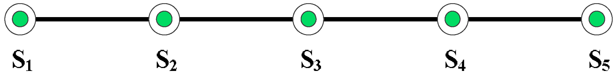
To describe the MML problem clearly, we construct a simple line network consisting of five nodes and four rail lines, which is shown in Figure 1.
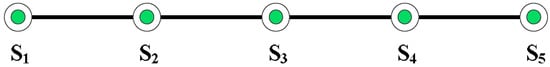
Figure 1.
A simple line railway network.
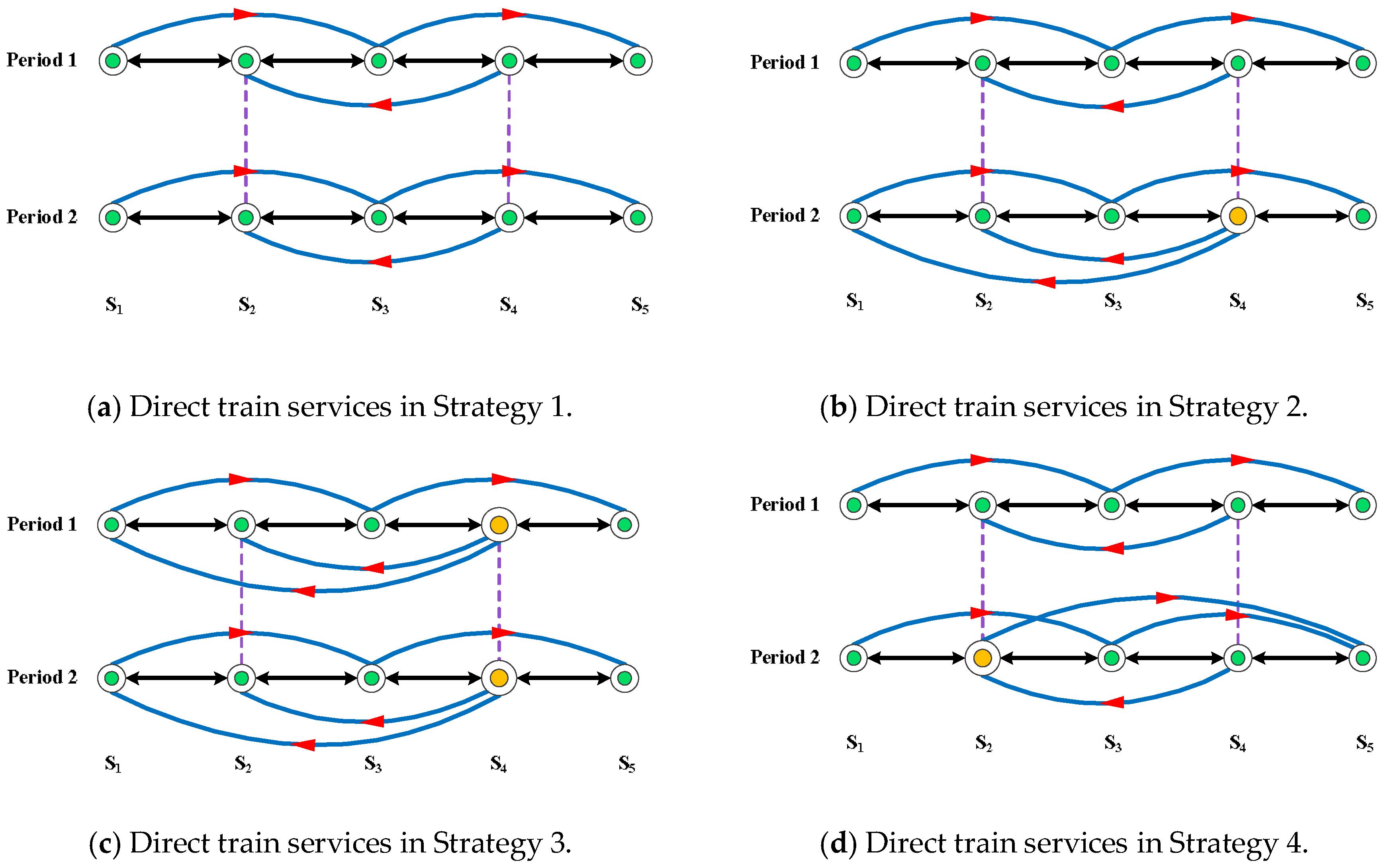
It is assumed that stations S1 through S5 are all SDLA yards, denoted as green circle, and S2 and S4 are candidate nodes for investment. For simplification, we analyze the MML problem in just two periods (Period 1 and Period 2). In addition, we assume that S2 and S4 both have two investment plans for selection in Period 1, including remaining as a SDLA yard and improved to a SDCO yard (expressed by yellow circle in Figure 2). It should be noted that, if the candidate yard remains a SDLA yard in Period 1, it still has two investment plans to choose in Period 2; otherwise, it can only remain a SDCO yard in Period 2, i.e., yard downsizing and closure are not considered (SDLASDCO is feasible, not vice versa). Moreover, we assume that the budget in each period is only enough for expanding one candidate yard from SDLA to SDCO.

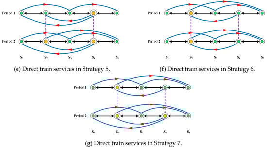
Figure 2.
Seven combinatorial strategies for investment.
As shown in Figure 2, there are seven combinatorial strategies. The train services between every two adjacent stations are created and expressed by a black solid line with two arrows, while the train services between non-adjacent stations are expressed by blue solid lines with red arrows, which constitute the optimal TCS plan together. In fact, improved yards are capable of handling more traffic flows with lower reclassification cost per car, and creating more blocks simultaneously. In this context, part of shipments originally reclassified at high-cost yards might be transferred to low-cost yards, and more train services might be provided. Therefore, the optimum TCS plan of a network might change with the spatial configuration of yards.
Strategy 1 (see Figure 2a): None of the candidate stations are improved in two periods. In this case, the capital investment is the lowest, while the total operating cost is the highest. There are only three train services between non-adjacent stations, namely, , and .
Strategy 2 (see Figure 2b): Although station S4 remains a SDLA yard in Period 1, it is expanded to a SDCO yard in Period 2. However, no capital is invested to station S2 in both two periods. A new train connection service is provided in Period 2 on the basis of Strategy 1.
Strategy 3 (see Figure 2c): Station S4 is expanded to a SDCO yard in Period 1 and remains a SDCO yard in Period 2. Station S2 remains a SDLA yard in two periods. The capital investment of this strategy is equal to that of Strategy 2. As a more efficient yard S4 comes into use since Period 1, the total operation cost of Strategy 3 is lower than Strategy 2. Additionally, a Strategy 1-based new train service is created in both periods.
Strategy 4 (see Figure 2d): Only station S2 is improved to a SDCO yard in Period 2. And a new direct train service is provided in Period 2 in comparison with Strategy 1.
Strategy 5 (see Figure 2e): S2 is improved to a SDCO yard in Period 2, and S4 is expanded to a SDCO yard in Period 1. In this case, a new direct train service is provided in both periods, and another new train service is added in Period 2 based on Strategy 1.
Strategy 6 (see Figure 2f): Station S2 is expanded to a SDCO yard in Period 1, while station S4 remains a SDLA yard throughout the planning horizon. The capital investment of this strategy is equal to Strategy 4, but the total operation cost is lower than Strategy 4. Two periods of Strategy 6 share the common train services and a new service is added on the basis of Strategy 1.
Strategy 7 (see Figure 2g): In contrast to Strategy 5, S2 is improved to a SDCO yard in Period 1, and S4 is expanded to a SDCO yard in Period 2. In this context, a new direct train service is provided both in Period 1 and Period 2, and another new train service is created in Period 2 based on Strategy 1. This strategy calls for the equivalent capital investment of Strategy 5.
3.2. Analysis of Two Extreme Combinatorial Strategies of the Multi-Period and Multi-Classification-Yard Location Problem
- (1)
- None of the candidate stations are invested in the whole planning horizon. This strategy calls for the minimum capital investment. However, the total operation cost is at the highest level due to the highest unit reclassification cost in average. Moreover, congestion may occur at some yards as the classification capacity of yards does not necessarily meet the increasing OD demands.
- (2)
- All candidate stations are expanded to their largest scale at the first period. Although this strategy significantly reduces the operation cost and satisfies the demands of all shipments, it calls for a significant amount of capital investment, which quite possibly exceeds the budget, and results in a huge waste of resources.
It should be noted that the solution to the MML problem is a trade-off between capital investment and operation cost. The evaluation of this trade-off is the core of our study.
3.3. The Complexity of Multi-Period and Multi-Classification-Yard Location Problem
The number of combinatorial investment strategies grows exponentially with the number of candidate nodes and periods. For a network containing five candidate nodes, if each of them has three optional investment plans in each period, then the number of combinatorial strategies (without consideration of budget constraint) will reach 243 for one period, 59,049 for two periods, 14,348,907 for three periods, and over 3.4 billion for four periods. Furthermore, each investment strategy is involved with a TCS problem, which is also a very challenging problem. For instance, there are 10 combinations for routing shipments over a line network with four yards, 150 for five yards, 7800 for six yards, 1,575,600 for seven yards, and over 1.3 billion for eight yards (Lin et al. [23]). Therefore, the MML problem is highly complex.
4. Mathematical Model
In this section, we formulate a bi-level programming model for the MML problem. The upper-level aims to find an optimal investment strategy for candidate nodes, i.e., which type of yards should the candidate nodes be built into or improved to. The lower-level is intended to obtain a least costly train connecting service plan, considering reclassification cost and accumulation delay. The model is constrained by capital budget, classification capacity, the number of available tracks, etc. For simplification, following assumptions are made in this paper.
Assumption 1.
We assume that train services must be provided between adjacent stations. It simplifies the problem by avoiding considering which pairs of adjacent stations should be provided with train services, hence reducing the complexity in making train formation plans to some extent. In fact, as positive traffic flows do not necessarily exist between every two adjacent stations, there might be no train services between some of them, in practice. To relax this assumption, the train services between adjacent stations should also be treated as variables.
Assumption 2.
It is assumed that the physical path of each OD demand is predefined. Although this is a standard practice used in China railway system in making a TCS plan, it might result in a higher operation cost compared with joint optimization of railcar itinerary and train formation plan. One solution to this problem is to optimize train paths and railcar reclassification plans simultaneously.
Assumption 3.
We assume that candidate nodes can only be built into new yards or improved to larger yards, i.e., yard downsizing and closure are not permitted. This assumption simplifies the problem by excluding many combinatorial investment strategies. In the real world, with the configuration change of yards, the workload of some yards might decline dramatically, which might be closed or downsized by railroad for optimization. To relax this assumption, we should consider yard downsizing and closure as potential plans for candidate yards.
4.1. Notations
The notations used in this paper are listed in Table 2.
Table 2.
Notations used in this paper.
4.2. Model Descriptions
In each period, only one investment plan can be selected for each candidate node, which can be described by
It should be noted that, in the first period, if , then . In addition, according to Assumption 3, if the yard scale corresponding to plan is smaller than , then . Additionally, a logical constraint indicating the relation of selected plans in consecutive periods should be considered:
The daily operation cost of all nodes, including accumulation delay and reclassification cost, is denoted by , which is converted to the PDV by :
Therefore, an upper-level formulation can be constructed to describe the MML problem:
Upper-level program:
The first term of the objective function is the capital investment for all candidate nodes throughout the planning horizon. The second term is the PDV of total operation cost of nodes in all periods. The constraint (7) ensures that the capital investment would not exceed the budget in each period. Apparently, without consideration of the operation cost reduction due to yard establishment or improvement, the upper-level reaches its optimality when the investment for all candidate nodes is zero. In fact, building or improving a yard will not only increase the classification capacity and the number of tracks, but also raise operation efficiency and reduce classification cost, significantly affecting the routing of car flows over the network. Therefore, the selection of investment strategies for candidate yard locations can be viewed as a location problem, while the determination of train connecting services and distribution of classification workload can be referred as an allocation problem. If a direct train service is provided between two yards, then an accumulation delay will be incurred at the origin yard. Note that, the charge of providing a train service is related to the size of train, rather than traffic volume (details can be referred to Lin et al. [23]). If some shipments are reclassified at yard , reclassification cost will be incurred.
The workload of node in period , i.e., the number of cars reclassified at node per day in period , can be expressed by
Then, the service flow from to in period , which is equivalent to the number of cars shipped by train service , can be expressed by
In this way, the lower-level program can be expressed by
Lower-level program:
The objective function of the lower-level consists of three terms. The first term is the total accumulation delay of all train services. The second term is the classification cost of yards not included in , while the third term is the classification cost of nodes included in .
The constraint (12) guarantees that a car flow can either be directly shipped to the destination or classified at not less than one intermediate yard on its itinerary in each period. The constraint (13) ensures that if a car flow from to is initially reclassified at yard , there must be a direct train service from to . The constraint (14) guarantees that the volume of car flows from to , carried by direct trains or reclassified at one or more yards on their itinerary, is equal to the total volume of (railcars which originate at and are destined to in period ), and the railcars which are reclassified at and destined to . The constraints (15) and (16) are logical constraints, indicating the relations between and , , and , respectively. For example, if , there will be no direct train service from to in period , and no shipments will be directly shipped from to in this period, i.e., . By contrast, if , the shipments from to will be delivered by direct trains. As is less than the total traffic volume in the network, hence, (where is a large enough positive number). It should be noted that, one classification track can generally store, at most, 200 railcars which are destined to other yards, simultaneously, in practice. In this case, the constraints (19) and (20) imply the relation between service flow and the number of tracks needed. For the nodes not included in , the constraint (21) ensures that the workload would not exceed their available classification capacity, and the constraint (23) guarantees that the number of used tracks is less than the number of available tracks. Similarly, for the nodes included in , the constraint (22) states that the capacity of these nodes is large enough to handle the traffic flows after possible establishment or improvement, and the constraint (24) represents that there are enough classification tracks for storing railcars in each period after possible investment.
In fact, the vast majority of car flows originating at yard is actually obtained by aggregating the shipments from the small stations around yard (see Lin et al. [23] for details). In the process of aggregation, these shipments should be reclassified and assigned to classification tracks (the storage capacity of this type of track is about 200 railcars in practice), together with car flows from other yards. Similarly, when the shipments arrive at the destination yard , they should also be reclassified and assigned to the tracks reserved specially for them (the capacity of this type of track is usually set to 150 railcars), and then delivered to the final destinations (small stations surrounding yard ) by local trains (with smaller train size and higher frequency).
5. Numerical Studies
In this section, a numerical example is carried out test our method, on the basis of a small railway network containing nine yards, and the results are subsequently analyzed.
5.1. The Input Data
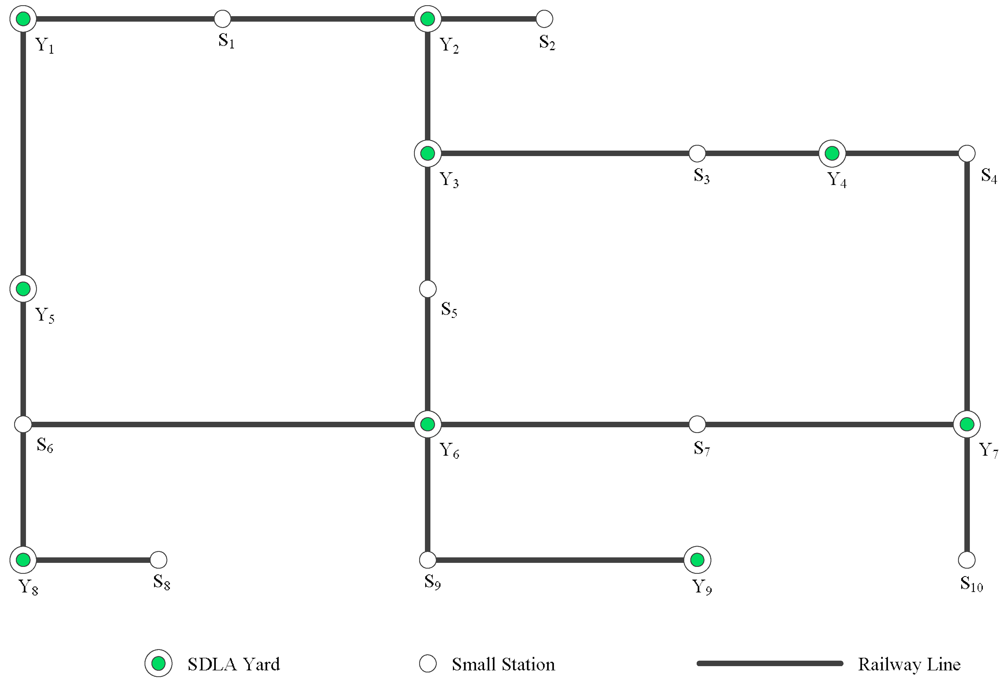
To test the effectiveness and validity of our model, a small railway network containing nine yards (denoted Y1 through Y9) and ten small stations (denoted S1 through S10) is constructed (see Figure 3). It is assumed that these nine yards are all SDLA yards at present, while nine stations have no classification capacity. The parameters of nine yards, such as accumulation parameter, classification cost per railcar, etc., are listed in Table 3.
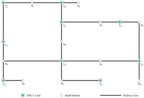
Figure 3.
A small railway network.
Table 3.
The parameters of nine yards.
For simplification, Y3 and Y6 are defined as two candidate yards for improvement, and we intend to obtain the optimal investment strategy in just two periods. The OD demands (the number of railcars from origin to destination per day in average) in Period 1 and Period 2 are shown in Table 4 and Table 5, respectively, and the physical path (listed in Appendix A) of each OD pair is specified in advance, which is a standard practice in China railway system, thus, the operation mileage in total is a constant.
Table 4.
The OD matrix in Period 1 (car per day).
Table 5.
The OD matrix in Period 2 (car per day).
We assume that both Y3 and Y6 have three investment plans as options, which are remaining a SDLA yard, improved to a SDCO yard, and expanded to a SDLO yard, respectively, i.e., , . As we do not take yard downsizing and closure into consideration, there are six combinations that might occur for each candidate yard in two periods. The capital investment, increase of classification capacity and track number, and decrease of unit classification cost of these combinations, are listed in Table 6.
Table 6.
Information of six investment combinations for a SDLA yard in two periods.
Furthermore, the budgets of investment in Period 1 and Period 2 are set to 1.5 billion CNY and 1.0 CNY respectively, i.e., , ; the time span of each period is set as five years, i.e., , ; the discount rate of capital investment is equal to 0.02 (); the coefficient is set to 20, i.e., the economic cost of one car-hour is equivalent to 20 CNY; and the proportional factor of classification capacity and tracks for nine yards are all set to 0.9 (). In addition, OD demands satisfying the sufficient condition for providing a train service, that they must be delivered to their destinations directly without optimization. The sufficient condition can be described as follows:
where denotes a minimum classification cost of yards on the itinerary of shipment , i.e.,
In other words, if shipment is reclassified at a certain intermediate yard with minimum relative delay on its itinerary, and the classification cost is greater than the cost of dispatching direct trains, then a direct train service should be provided without optimization.
5.2. Results and Discussion
The MML problem mentioned above is solved by Gurobi 7.5.2 on a 2.20 GHz Intel (R) Core (TM) i5-5200U CPU computer with 4.0 GB of RAM. As each yard has six investment combinations in total throughout the planning horizon, there are 36 () combinatorial investment strategies for two yards, in theory. However, in light of the budget constraints in two periods, there are only 17 strategies that are available, whose capital investment, operation cost, etc., are listed below.
As shown in Table 7, Strategy 3 is the optimal one with a minimum total cost of 2.643 billion CNY. In this strategy, yard Y3 remains a SDLA yard in two periods, while yard Y6 is expanded to a SDCO yard in Period 1 and remains unchanged in Period 2. The capital investment of this strategy is 0.7 billion CNY, and the overall operation cost of nine yards in two periods is equal to 1.943 billion CNY. Additionally, the daily workload and track utilization of nine yards in two periods are shown in Table 8.
Table 7.
The cost of available combinatorial strategies.
Table 8.
Workload and track utilization of nine yards.
In Table 8, the available capacity of a certain yard is obtained by classification capacity in total minus the capacity reserved for local car flows, which can be expressed by
Similarly, the available track number of a certain yard is equal to the total tracks minus the tracks reserved for arrival car flows, which can be expressed by
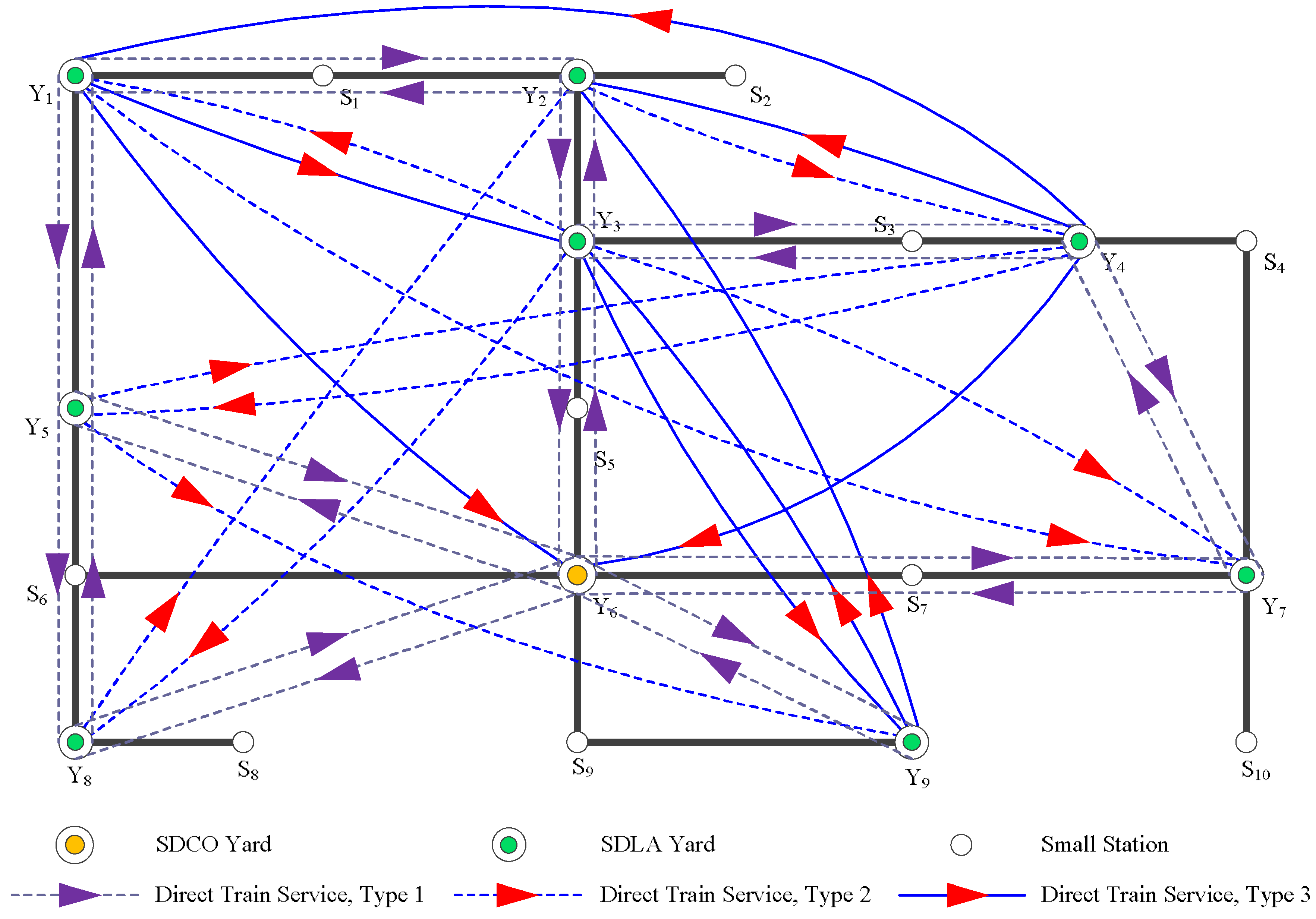
As shown in Table 8, the workload of yards Y7, Y8, and Y9 are equal to zero both in Period 1 and Period 2. This is because no car flow passes through these yards according to the predefined physical paths (i.e., none of them is intermediate yard). In addition, the workload of yards Y2 and Y4 decrease to zero in Period 2. This is mainly due to the increase of car flow volume, i.e., it is more favorable to provide more direct trains than reclassify railcars at Y2 and Y4. The train connection services in the railway network in Period 1 are depicted in Figure 4.

Figure 4.
Direct train services among nine yards in Period 1.
Theoretically, the potential train services for nine yards are 72 (). However, in Figure 2, there are only 39 direct train services provided in this railway network, 22 of which are created between adjacent yards (Type 1 service); nine of which satisfy the sufficient condition (Type 2 service); and eight of which are obtained by the optimization from the remaining 41 potential train services (Type 3 service). Table 9 lists all the direct train services, and the volume of and in Period 1, while Table 10 lists all the car flow variables and corresponding traffic volume in Period 1.
Table 9.
Information of direct train services in Period 1.
Table 10.
Car flow variable and corresponding traffic flow volume in Period 1.
As shown in Table 9, the direct train service with maximum traffic volume is Y6→Y9, whose service flow is up to 455.07 cars per day, i.e., on average dispatching 9.1 (455.07/50) trains each day. Conversely, the direct train service with minimum volume is Y8→Y5, whose service flow is just 44.73 cars per day, less than one train per day.
Additionally, the reclassification strategy of each OD demand can be obtained on the basis of Table 9 and Table 10. For example, to get the reclassification strategy of the OD demand , we should first determine whether direct train service Y1→Y9 exists in Table 9. If the answer is NO, then we turn to Table 10. It can be found that car flow variable (Y1, Y6, Y9) exists in Table 10, which indicates that shipment will be first reclassified at classification yard Y6, and merged into the car flow from Y6 to Y9. Next, we look up Table 10 to determine whether train service Y6→Y9 exists or not. Obviously, the answer is YES, i.e., will be consolidated into the direct train service Y6→Y9 at yard Y6 and delivered to its destination Y9. Finally, the reclassification strategy of OD demand is Y1→Y6→Y9.
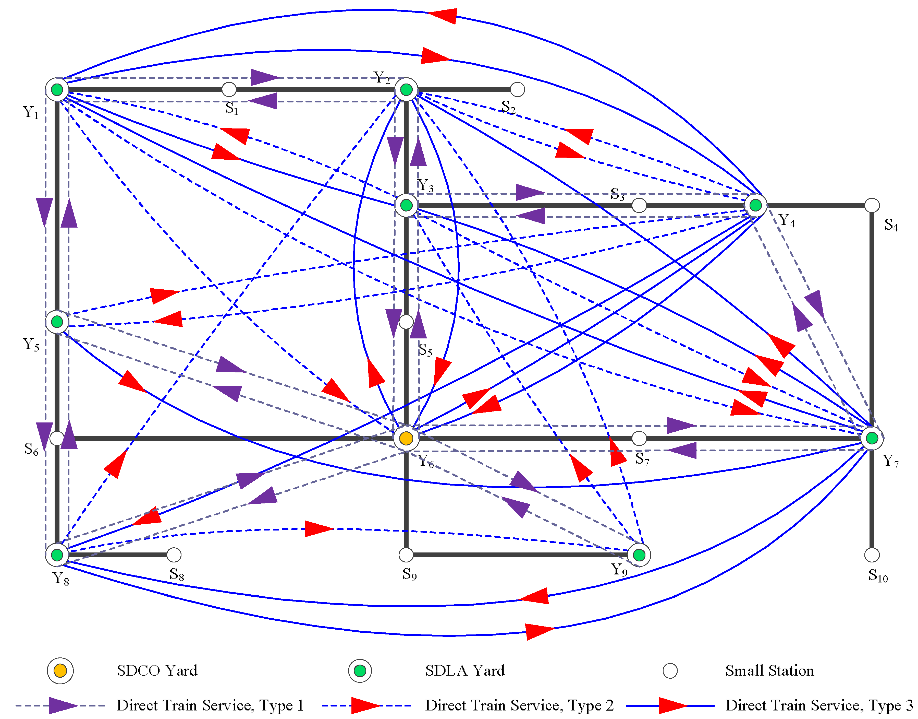
Figure 5 depicts all the direct train services (48 services) provided in Period 2, 12 of which satisfy the sufficient condition; 22 of which are created between adjacent yards; and 14 of which are obtained by the optimization from the remaining 38 train services.
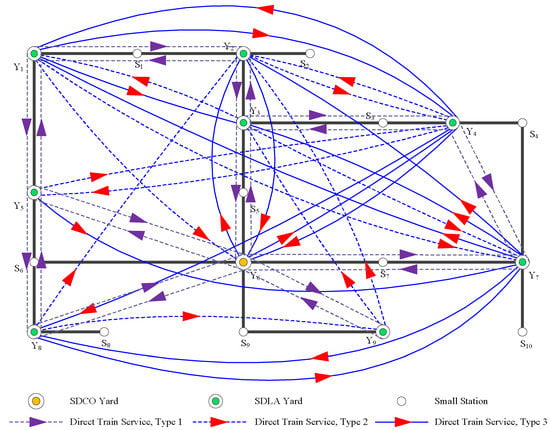
Figure 5.
Direct train services among nine yards in Period 2.
Table 11 lists all the direct train services, and the volume of and in Period 2, while Table 12 lists all the car flow variables and corresponding traffic volume in Period 2.
Table 11.
Information of direct train services in Period 2.
Table 12.
Car flow variable and corresponding traffic flow in Period 2.
In Table 11, the direct train service with maximum traffic volume is Y9→Y6, reaching 488.94 cars per day, i.e., on average dispatching 9.8 (488.94/50) trains each day. In contrast, the direct train service with minimum traffic volume is Y4→Y3, whose service flow is just 34.84 cars per day, less than one train per day. The reclassification strategies of OD demands in Period 2 can also be obtained by the method mentioned above.
6. Conclusions
In this paper, we formulate the MML problem as a multi-period location–allocation problem with railway characteristics, and established a bi-level programming model constrained by budget, classification capacity, and number of available tracks. The upper-level is intended to find an optimal combinatorial investment strategy for all candidate nodes throughout the planning horizon, and the lower-level aims to obtain a least costly railcar reclassification plan on the basis of the strategy given by the upper-level. In light of the economies of scale in yard establishment and improvement, and the highly-nonlinear interrelation among yards, the investment strategy should be analyzed from the perspective of the entire planning horizon and the whole railway network, rather than focusing on a certain period or a certain yard. To test the effectiveness and validity of our model, a numerical study with two candidate yards in two periods is carried out and solved by using Gurobi 7.5.2. In the optimal investment strategy we obtained, i.e., yard Y3 remains a SDLA yard in two periods, while yard Y6 is expanded to a SDCO yard in Period 1 and remains unchanged in Period 2, all the yards can handle their workload in the near future and keep an appropriate capacity utilization ratio, which indicates that the proposed model can serve as a solid aid in the decision-making of classification yard location. With the building of new railway lines, such as Lanzhou–Chongqing Railway and Afuzhun Railway, some yards might be improved to match with the expanded railway network. In this case, railway departments might achieve substantial cost savings by applying our method in their five-year plans for yard improvement.
In the long term, researchers can focus on the simultaneously addressing of car flow routing and classification yards location. We identify this a promising area for future research.
Author Contributions
The authors contributed equally to this work.
Acknowledgments
This work was supported by the China Railway under Grant Number, 2002X25, 2004X008, 2004F022; the science technology and legal department of the National Railway Administration of the People’s Republic of China under Grant Number, KF2017-015 and China Railway First Survey and Design Institute Group Co., Ltd. under Grant Number, 13-03-1.
Conflicts of Interest
The authors declare no conflict of interest.
Appendix A. The Physical Paths of OD Demands
| No. | Origin | Destination | Physical Path | No. | Origin | Destination | Physical Path |
| 1 | Y1 | Y2 | Y1→Y2 | 37 | Y5 | Y6 | Y5→Y6 |
| 2 | Y1 | Y3 | Y1→Y2→Y3 | 38 | Y5 | Y7 | Y5→Y6→Y7 |
| 3 | Y1 | Y4 | Y1→Y2→Y3→Y4 | 39 | Y5 | Y8 | Y5→Y8 |
| 4 | Y1 | Y5 | Y1→Y5 | 40 | Y5 | Y9 | Y5→Y6→Y9 |
| 5 | Y1 | Y6 | Y1→Y2→Y3→Y6 | 41 | Y6 | Y1 | Y6→Y3→Y2→Y1 |
| 6 | Y1 | Y7 | Y1→Y2→Y3→Y4→Y7 | 42 | Y6 | Y2 | Y6→Y3→Y2 |
| 7 | Y1 | Y8 | Y1→Y5→Y8 | 43 | Y6 | Y3 | Y6→Y3 |
| 8 | Y1 | Y9 | Y1→Y2→Y3→Y6→Y9 | 44 | Y6 | Y4 | Y6→Y3→Y4 |
| 9 | Y2 | Y1 | Y2→Y1 | 45 | Y6 | Y5 | Y6→Y5 |
| 10 | Y2 | Y3 | Y2→Y3 | 46 | Y6 | Y7 | Y6→Y7 |
| 11 | Y2 | Y4 | Y2→Y3→Y4 | 47 | Y6 | Y8 | Y6→Y8 |
| 12 | Y2 | Y5 | Y2→Y1→Y5 | 48 | Y6 | Y9 | Y6→Y9 |
| 13 | Y2 | Y6 | Y2→Y3→Y6 | 49 | Y7 | Y1 | Y7→Y4→Y3→Y2→Y1 |
| 14 | Y2 | Y7 | Y2→Y3→Y4→Y7 | 50 | Y7 | Y2 | Y7→Y4→Y3→Y2 |
| 15 | Y2 | Y8 | Y2→Y1→Y5→Y8 | 51 | Y7 | Y3 | Y7→Y4→Y3 |
| 16 | Y2 | Y9 | Y2→Y3→Y6→Y9 | 52 | Y7 | Y4 | Y7→Y4 |
| 17 | Y3 | Y1 | Y3→Y2→Y1 | 53 | Y7 | Y5 | Y7→Y6→Y5 |
| 18 | Y3 | Y2 | Y3→Y2 | 54 | Y7 | Y6 | Y7→Y6 |
| 19 | Y3 | Y4 | Y3→Y4 | 55 | Y7 | Y8 | Y7→Y6→Y8 |
| 20 | Y3 | Y5 | Y3→Y2→Y1→Y5 | 56 | Y7 | Y9 | Y7→Y6→Y9 |
| 21 | Y3 | Y6 | Y3→Y6 | 57 | Y8 | Y1 | Y8→Y5→Y1 |
| 22 | Y3 | Y7 | Y3→Y4→Y7 | 58 | Y8 | Y2 | Y8→Y5→Y1→Y2 |
| 23 | Y3 | Y8 | Y3→Y6→Y8 | 59 | Y8 | Y3 | Y8→Y6→Y3 |
| 24 | Y3 | Y9 | Y3→Y6→Y9 | 60 | Y8 | Y4 | Y8→Y6→Y3→Y4 |
| 25 | Y4 | Y1 | Y4→Y3→Y2→Y1 | 61 | Y8 | Y5 | Y8→Y5 |
| 26 | Y4 | Y2 | Y4→Y3→Y2 | 62 | Y8 | Y6 | Y8→Y6 |
| 27 | Y4 | Y3 | Y4→Y3 | 63 | Y8 | Y7 | Y8→Y6→Y7 |
| 28 | Y4 | Y5 | Y4→Y3→Y2→Y1→Y5 | 64 | Y8 | Y9 | Y8→Y6→Y9 |
| 29 | Y4 | Y6 | Y4→Y3→Y6 | 65 | Y9 | Y1 | Y9→Y6→Y3→Y2→Y1 |
| 30 | Y4 | Y7 | Y4→Y7 | 66 | Y9 | Y2 | Y9→Y6→Y3→Y2 |
| 31 | Y4 | Y8 | Y4→Y3→Y6→Y8 | 67 | Y9 | Y3 | Y9→Y6→Y3 |
| 32 | Y4 | Y9 | Y4→Y3→Y6→Y9 | 68 | Y9 | Y4 | Y9→Y6→Y3→Y4 |
| 33 | Y5 | Y1 | Y5→Y1 | 69 | Y9 | Y5 | Y9→Y6→Y5 |
| 34 | Y5 | Y2 | Y5→Y1→Y2 | 70 | Y9 | Y6 | Y9→Y6 |
| 35 | Y5 | Y3 | Y5→Y1→Y2→Y3 | 71 | Y9 | Y7 | Y9→Y6→Y7 |
| 36 | Y5 | Y4 | Y5→Y1→Y2→Y3→Y4 | 72 | Y9 | Y8 | Y9→Y6→Y8 |
References
- Cooper, L. Location-allocation problems. Oper. Res. 1963, 11, 331–343. [Google Scholar] [CrossRef]
- Bongartz, I.; Calamai, P.H.; Conn, A.R. A projection method for lp norm location-allocation problems. Math. Program. 1994, 66, 283–312. [Google Scholar] [CrossRef]
- Eben-Chaime, M.; Mehrez, A.; Markovich, G. Capacitated location-allocation problems on a line. Comput. Oper. Res. 2002, 29, 459–470. [Google Scholar] [CrossRef]
- Brimberg, J.; Hansen, P.; Mladenović, N.; Salhi, S. A survey of solution methods for the continuous location-allocation problem. Int. J. Oper. Res. 2008, 5, 1–12. [Google Scholar]
- Manzini, R.; Gebennini, E. Optimization models for the dynamic facility location and allocation problem. Int. J. Prod. Res. 2008, 46, 2061–2086. [Google Scholar] [CrossRef]
- Gokbayrak, K.; Kocaman, A.S. A Distance-limited continuous location-allocation problem for spatial planning of decentralized systems. Comput. Oper. Res. 2017, 88, 15–29. [Google Scholar] [CrossRef]
- Gupta, R.; Muttoo, S.K.; Pal, S.K. Fuzzy c-means clustering and particle swarm optimization based scheme for common service center location allocation. Appl. Intell. 2017, 47, 624–643. [Google Scholar] [CrossRef]
- Cebecauer, M.; Buzna, L. A versatile adaptive aggregation framework for spatially large discrete location-allocation problems. Comput. Ind. Eng. 2017, 111, 364–380. [Google Scholar] [CrossRef]
- Wesolowsky, G.O.; Truscott, W.G. The multiperiod location-allocation problem with relocation of facilities. Manag. Sci. 1975, 22, 57–65. [Google Scholar] [CrossRef]
- Hinojosa, Y.; Puerto, J.; Fernández, F.R. A multiperiod two-echelon multicommodity capacitated plant location problem. Eur. J. Oper. Res. 2000, 123, 271–291. [Google Scholar] [CrossRef]
- Canel, C.; Khumawala, B.M.; Law, J.; Loh, A. An algorithm for the capacitated, multi-commodity multi-period facility location problem. Comput. Oper. Res. 2001, 28, 411–427. [Google Scholar] [CrossRef]
- Rajagopalan, H.K.; Saydam, C.; Xiao, J. A multiperiod set covering location model for dynamic redeployment of ambulances. Comput. Oper. Res. 2008, 35, 814–826. [Google Scholar] [CrossRef]
- Klibi, W.; Lasalle, F.; Martel, A.; Ichoua, S. The stochastic multiperiod location transportation problem. Transp. Sci. 2010, 44, 221–237. [Google Scholar] [CrossRef]
- Sha, Y.; Huang, J. The multi-period location-allocation problem of engineering emergency blood supply systems. Syst. Eng. Proc. 2012, 5, 21–28. [Google Scholar] [CrossRef]
- Mansfield, E.; Wein, H.H. A model for the location of a railroad classification yard. Manag. Sci. 1958, 4, 292–313. [Google Scholar] [CrossRef]
- Assad, A.A. Models for rail transportation. Transp. Res. A-Pol. 1980, 14, 205–220. [Google Scholar] [CrossRef]
- Maji, A.; Jha, M.K. Railroad yard location optimization using a genetic algorithm. In Proceedings of the 2nd WSEAS International Conference on Natural Hazards; 2nd International Conference on Climate Changes, Global Warming, Biological Programs; 2nd International Conference on Urban Rehabil and Sustainable, Baltimore, MD, USA, 7–9 November 2009; World Scientific and Engineering Academic and Society: Athens, Greece, 2009; pp. 151–156. [Google Scholar]
- Lee, J.S.; Kim, D.K.; Chon, K.S. Design of optimal marshalling yard location model considering rail freight hub network properties. In Proceedings of the International Conference on Eastern Asia Society for Transportation Studies, Dalian, China, 24–27 September 2007; pp. 1031–1045. [Google Scholar]
- Lin, B.L.; Xu, Z.Y.; Huang, M.; Ji, J.L.; Guo, P.W. An optimization approach to railroad classification yard location and installment size decision with budget constraint. J. Chin. Railw. Soc. 2002, 24, 5–8. [Google Scholar] [CrossRef]
- Yan, H.X.; Lin, B.L.; Zheng, J.R.; Zhang, Y.H. Comparative study on optimal type selection of marshalling station between unidirectional and bidirectional. J. Transp. Syst. Eng. Inf. Tech. 2007, 7, 124–131. [Google Scholar] [CrossRef]
- Li, H.D.; He, S.W.; Song, R.; Ji, L.J.; Shen, Y.S. Synthetic optimization of train formation plan and layout of technical service station. J. Beijing Jiaotong Univ. 2010, 34, 30–34. [Google Scholar] [CrossRef]
- Geng, L.Q. Optimization model of freight car marshalling scheme and load dividing and combining in marshalling station. Railw. Transp. Econ. 2011, 33, 59–63. [Google Scholar] [CrossRef]
- Lin, B.L.; Wang, Z.M.; Ji, L.J.; Tian, Y.M.; Zhou, G.Q. Optimizing the freight train connection service network of a large-scale rail system. Transp. Res. B-Methodol. 2012, 46, 649–667. [Google Scholar] [CrossRef]
© 2018 by the authors. Licensee MDPI, Basel, Switzerland. This article is an open access article distributed under the terms and conditions of the Creative Commons Attribution (CC BY) license (http://creativecommons.org/licenses/by/4.0/).