Convolutional Neural Network for Copy-Move Forgery Detection

Abstract

Digital image forgery is a growing problem due to the increase in readily-available technology that makes the process relatively easy. In response, several approaches have been developed for detecting digital forgeries. This paper proposes a novel scheme based on neural networks and deep learning, focusing on the convolutional neural network (CNN) architecture approach to enhance a copy-move forgery detection. The proposed approach employs a CNN architecture that incorporates pre-processing layers to give satisfactory results. In addition, the possibility of using this model for various copy-move forgery techniques is explained. The experiments show that the overall validation accuracy is 90%, with a set iteration limit.

1. Introduction

Digital editing is becoming less and less complicated with time, as a result of the increased availability of a wide array of digital image editing tools. Image forgery, which is defined as “the process of cropping and pasting regions on the same or separate sources [1], is one of the most popular forms of digital editing. Copy-move forgery detection technology can be applied as a means to measure an image’s authenticity. This is done through the detection of “clues” that are typically found in copy-move forged images.

In the field of digital image forensics, copy-move forgery detection generally falls into two categories: keypoint-based and block-based [2]. This paper will focus on the latter category. Block-based copy-move forgery detection approaches employ image patches that overlap. From these, “raw” pixels are removed for forgery testing against similar patches [3]. Of the many strategies currently being employed in image forgery detection, several use statistical characteristics across a variety of domains [4]. Regardless of the forgery category, the forgery detection application will deal with active image copy-move forgery and/or passive copy-move forgery. In the former type, the original image includes embedded valuable data which makes the detection process easier, whereas in the latter, the original is imaging that makes the detection more challenging and difficult. Image forgery localization is even more difficult to carry out [5]. While forgery detection only seeks to know if an image is in whole or in part fake or original, image forgery localization tries to find the exact forged portions [5].

Furthermore, in image forgery localization, the focus is on building a model rather than looking at only certain features or domains. The model will be used to automatically detect specific elements based on a form of advanced deep neural network. Examples of these types of networks include deep belief network [6], deep auto encoder [7], and convolutional neural network (CNN) [8]. Of these three neural networks, CNNs are most commonly used in vision applications. These approaches employ local neighborhood pooling operations and trainable filters when testing raw input images, thereby creating hierarchies (from concrete to abstract) of the features under examination. Because the image analysis and computer vision in the CNN strategy are so highly advanced, CNN generally provides excellent performance [9,10] in image forgery detection, through the composition of simplistic non-linear and linear filtering operations (e.g., rectification and convolution) [11].

This present paper proposes a novel approach for image forgery detection and localization which is based on scale variant convolutional neural networks (SVCNNs). An outline of the proposed method is presented in Figure 3. For this approach, sliding windows that incorporate a variety of scales are included in customized CNNs with the aim of creating possibility maps that indicate image tampering. Our main focus is both copy-move forgery detection and localization through the application of elements removed via the use of CNNs.

The rest of the paper is organized as follows. In Section 2, we introduce an overview of the literature that has contributed to the advancement of CNNs in copy-move forgery detection and feature extraction procedures. In Section 3, we introduce the proposed model and the training processes. In Section 4, the experiment’s environment and results are discussed. Finally, in Section 5, we present the study’s conclusions.

2. Related Work

This section provides an overview of related works in copy-move forgery detection using neural network CNN’s and related concepts.

CNN for forgery detection based on discrete cosine transformation (DCT): Numerous researchers have approached the problem using CNN’s for forgery detection. As discussed in [12], CNNs can be used in steganalysis for gray-scale images, where the CNNs first layer features a single high pass filter to filter out the image content. In [2], an image model is developed for detecting image-splicing detection. In this approach, the researchers used discrete cosine transformation (DCT), to remove relevant features out of the DCT domain [2].

The DCT domain feeds the input of the CNN by transferring the row of quantized DCT coefficients from the JPEG file to data classification. The processing of the data in the classification stage will generate a histogram for each patch and concatenate all of the histograms to feed the CNN [13].

In [14,15,16] deep learning methods applied to computer vision problems resulted in a local convolution feature data-driven CNN, while in other research, copy-move forgery detection algorithms were mostly based on computer vision tasks such as image retrieval [17,18], classification [19], and object detection [20].

Along with CNN, graphics processing unit (GPU) technologies have helped to fuel the latest improvements in computer vision tasks [14]. Unlike traditional strategies for image classification, which mostly use local descriptors [21], the latest CNN-based image classification techniques use end-to-end structure. Because deep networks typically incorporate classifiers and features that are high, mid, or low level [22] using end-on-end multilayers, the various feature levels are enriched according to the number of hidden layers. The most recent convolutional neural networks (e.g., VGG (Convolutional network for classification and detection) [12,14,16,23,24], significantly enhance performance in object detection and image classification tasks [15]. Table 1 provides a brief summary of some common CNNs [25].

Table 1. The common convolutional neural network (CNNs) characteristics.

CNN		Layers No.	Inventor(s)	Year	Place	Parameters No.	Error Rate
[25]	LeNet	8	Yann LeCun	1988	First	60 T	N/A
[14]	AlexNet	7	Alex Kirzhevsky Hinton, Ilya Sutskever	2012	First	60 M	15.3%
[22]	ZFNet	7	Matthew Zeiler and Rob Fergus	2013	First	N/A	14.8%
[25]	Google Net	9	Google	2014	First	4 M	6.67%
[23]	VGG Net	16	Simonyan, Zisserman	2014	Second	140 M	3.6%
[12]	ResNet	152	Kaiming He	2015	First	N/A	3.75%

In the CNNs mentioned above, the intermediate layers serve as global features of image-level descriptors. This type of feature can reinforce inter-class differences but does not make any intra-class distinctions. The strategies for deep learning applied to computer vision tasks are also not suitable for direct use in copy-move forgery detection. As discussed previously, this kind of detection looks for the same types of regions that have been resized, rotated or deformed in some way. The expressive feature representations output derived from image-level CNNs [26] points to the possibility of using appropriate patch-level descriptors in order to replace handcrafted patch-level descriptors with data-driven ones [26].

The recent literature presents a number of deep local descriptors that offer impressive patch classification and matching abilities [27]. Because CNNs have been proven proficient in natural image distribution, they will likely also be useful in image copy-move forgery detection, given that the aim in that task is to find the so-called natural or pristine image among any unnatural or forged ones. The main key used to classify images in order to detect copy-move forgery and localize it is image features. Therefore, extracting image features is an essential part of the CNNs’ work in copy-move forgery detection. We will highlight the differences between the classic way and the CNN automatic way of feature extraction and show how the CNN strategy effectively eliminates the need for the first method.

2.1. Feature Extraction

The literature includes several different feature extraction approaches. Although the published works discuss a wide range of different strategies for detecting copy-move forgery, the present study will focus on three specific classifications of features, which are the polar cosine transforms (PCT), the Zernike moments (ZM), and the Fourier–Mellin transform (FMT). These three techniques are all similar in that they have circular harmonics transform expansions (CHT) which are more or less the same. This means that the CHT coefficient can be measured by image projection $I\left(\rho ,\theta \right)$, making use of the basis function $K_{n,m}\left(\rho ,\theta \right)$ for initiating the change, as given below:

$$F_I\left(n,m\right)={{\displaystyle \int }}_0^{\infty }\rho R_{n,m}^{*}\left(\rho \right)\times [\frac{1}{\sqrt{2\pi }}{{\displaystyle \int }}_0^{2\pi }I\left(\rho ,\theta \right)e^{-jm\theta }d\theta ]d\rho$$

(1)

As shown, the image $I\left(\rho ,\theta \right)$ occurs at the polar scheme, as $\rho \in \left[0,\infty \right]$ and $\theta \in \left[0,2\pi \right]$. Here, we can include elements from two expressions, as follows: 1). We can combine the Zernike radial with the function and $\rho$ value integration. 2). We can use brackets to show the Fourier series function which represents the image $I\left(\rho ,\theta \right)$ along with the phase term $e^{-jm\theta }$ and $\theta$ radians rotation. In this way, we can find rotation invariance and also apply coefficient magnitude. The absolute value of the FMT coefficient will then give scale invariance because any changes made to the image scale will increase the phase term. Consequently, the radial function thus becomes variant-based in accordance with feature designation and PCT radial functions which normalize coefficients $C_n$ and assert cosine functions ${\rho }^2$.

$$R_n\left(\rho \right)=C_n\cos \left(n\pi {\rho }^2\right)$$

(2)

Here, the Zernike radial function shows the same radial function as PCT. However, it also shows more suitable values for coefficients and gives the expression $\rho \in \left[0,1\right]$ for the two functions, as shown below:

$$R_{n,m}\left(\rho \right)={\displaystyle \sum }_{h=0}^{\left(n-\left|m\right|\right)/2}{C}_{n,m,h}{\rho }^{2-2h}$$

(3)

Additionally, we can express the FMT radial function as non-zero in $\rho \ge 0$, applying a constant value of $r$ against the ${\rho }^2$ value, as follows:

$$R_r\left(\rho \right)=\frac{1}{{\rho }^2}{e}^{jr\ln \left(\rho \right)}$$

(4)

These models are usable in patch size when featuring a good resolution. Therefore, to obtain more suitable matching using features in the two patches, the feature-length extension has to reside in a loose condition. Additionally, Cartesian and polar for ZM and PCT samples, respectively, need to be applied, but FMT will use log-polar for samples. In the present study, polar sampling will be used only for calculating rotation and scaling to obtain scalar values and optimized invariance angles [28].

2.2. Using CNNs for Feature Extraction

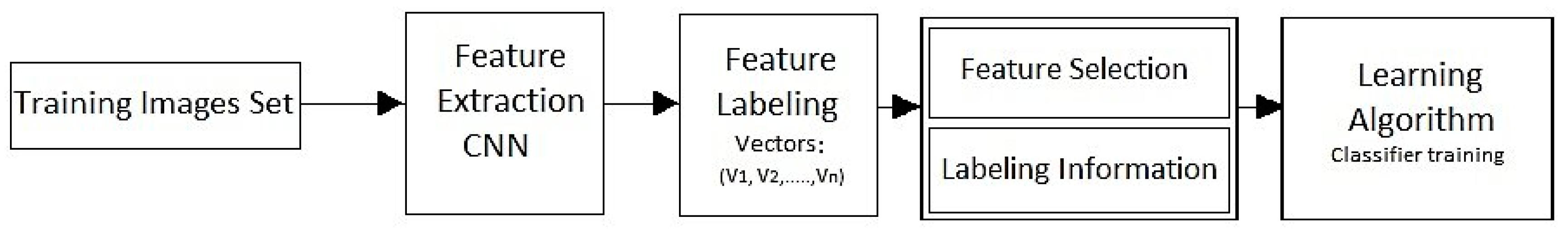
In neural networks, the process of feature extraction removes elements of learned images out of a pre-trained CNN (see Figure 1 and Figure 2). These images can then be utilized for training image classifiers. In general, feature extraction presents as the simplest approach when applying pretend deep networks of representational power as there is a clearly delineated hierarchy of the input images, which is easy to understand. In short, the deeper layers convey features of higher levels and are built by incorporating features from the lower levels found within earlier layers. Test and training images for feature representations can be sourced from previous fully-connected (FC) layers, while image representations from lower levels require an earlier network layer.

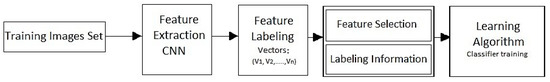
Figure 1. Feature selection for classification pipeline (the proposed model): training stage.

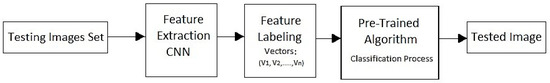
Figure 2. Feature selection for classification pipeline (the proposed model): testing stage.

2.3. Classifying Feature Selections

The last step for computer vision applications is to use feature selection in object identification to classify certain features according to specific characteristics. This stage is typically carried out using later layers of deep learning neural networks via a voting technique. Take, for example, the fully-connected layer known as learning. Because of a large amount of data, it can be challenging for the system to learn good classifiers prior to extracting undesirable features from the program. However, removing features which are irrelevant or repetitious creates a more generally applicable classifier and also serves to decrease learning algorithm run times, thus enabling a deeper understanding of the real-world problem to which the classifier is being applied.

A considerable amount of worthy research has already been conducted on existing techniques for detecting and localizing copy-move forgeries. The research has investigated whether these implemented methods are sufficiently robust and whether properly modeling the structural changes that have occurred in images due to copy-move forgeries can reliably classify a digital image as a pristine or manipulated image. Furthermore, many techniques of copy-move forgeries have been presented in the literature. Some good examples about detections techniques and their limitations are described by the authors of [29,30,31]. Some recent studies [29,30,31,32,33,34] on copy-move forgery detection have highlighted CNN’s that learn and minimize a loss function (an objective that scores the quality results) in an automatic process. However, many authors are still attempting manual efforts for designing effective loss function by telling the CNN what they wish to minimize [31,35].

3. The Proposed CNN Model

CNN’s are nonlinear interconnecting neurons based on the construct of the human visual system. Applying CNN’s for forensic purposes is a somewhat new approach, but their ability to segment images and identify objects is thus far unsurpassed [36]. In one study, where CNNs were used to extract input images’ features in order to classify them, the method outperformed all previous state-of-the-art approaches. Therefore, and based on the method from [36], our proposed CNN will be used as a feature extractor for image input patches in the training stage and, later on, for the testing stage as well (see Figure 2 and Figure 3). CNN’s can be deconstructed into building blocks known as layers. Layer $L_i$ will accept relevant input $H_i\times W_i\times P_i$ for feature maps or vectors sized as $P_i$. This layer then gives the output $H_{i+1}\times W_{i+1}\times P_{i+1}$ for feature maps or vectors sized as $P_{i+1}$. In the present study, we use six different kinds of layers: convolutional, pooling, ReLU, softmax, fully-connected, and batch normalization. A brief description of each type of these layers is given below.

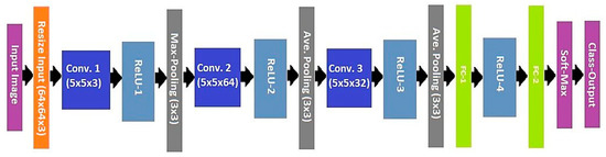
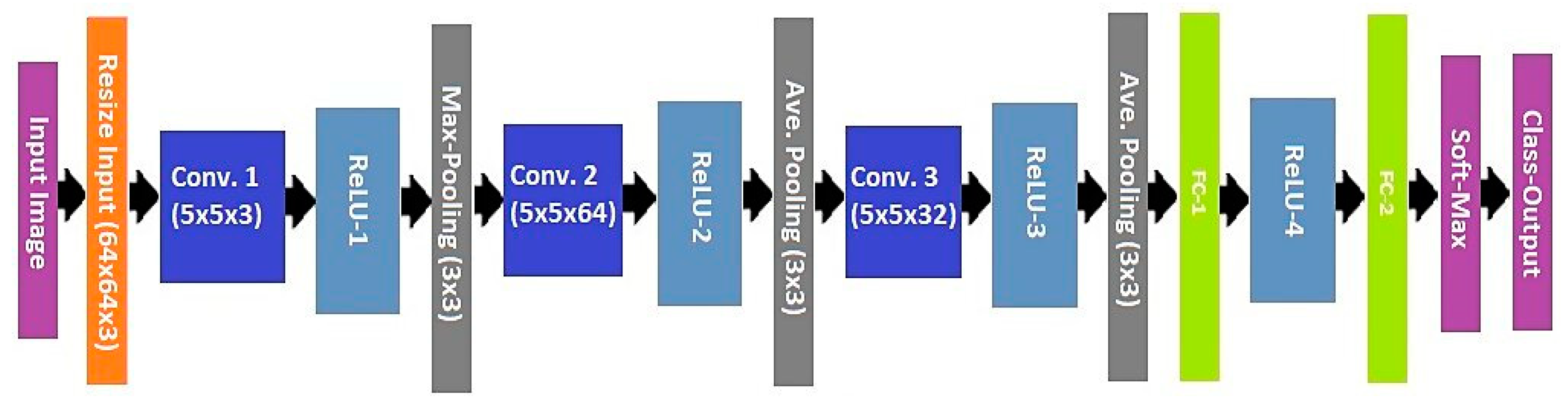
Figure 3. The architecture of the proposed CNN model.

(1)

In a convolutional layer, the convolutions are performed using stride $S_h$ and $S_w$ for the first two axes of the input feature maps, along with $P_{i+1}$ filters $K_h\times K_w\times P_i$ [37]:

$$H_{i+1}=\left[\frac{H_i-K_h+1}{S_h}\right]$$

(5)

$$W_{i+1}=\left[\frac{W_i-K_w+1}{S_w}\right]$$

(6)

$$P_{i+1}$$

(7)

(2)

In a pooling layer, which occurs following convolutions, the layer chooses pixel valuations of specific characteristics (e.g., average pooling or maximum pooling) within a given region. If a max-pooling layer is chosen, it then carries out maximum element extraction, i.e., stride $S_h$ and $S_w$ for the initial two axes in a neighborhood $K_h\times K_w$ for every two-dimensional piece of input the feature map. The input block’s maximum value is, therefore, returned [37]. This approach is commonly applied in deep learning networks. In our proposed strategy, the max-pooling layer will decrease the input image patch resolution, as well as enhance network robustness, in the face of possible valuation changes in the motion residuals of the frame’s absolute difference image [38].

$${\mathrm{H}}_{\mathrm{i}+1}=\left[\frac{{\mathrm{H}}_{\mathrm{i}}-{\mathrm{K}}_{\mathrm{h}}+1}{{\mathrm{S}}_{\mathrm{h}}}\right]$$

(8)

$${\mathrm{W}}_{\mathrm{i}+1}=\left[\frac{{\mathrm{W}}_{\mathrm{i}}-{\mathrm{K}}_{\mathrm{w}}+1}{{\mathrm{S}}_{\mathrm{w}}}\right]$$

(9)

$${\mathrm{P}}_{\mathrm{i}+1}={\mathrm{P}}_{\mathrm{i}}$$

(10)

Input image patches for CNN models use two-dimensional array image blocks measuring 3 × (64 × 64), with 3 indicating the channel number in the RGB-scale. Thus, if we use 3 × 3 as the window size and 3 as the stride size, then the image patch resolution decreases by half to 32 × 32 from its original 64 × 64, following the initial max-pooling layer [37].

(3)

ReLU layer performs element-wise nonlinear activation. Given a single neuron $x$, it is transformed into a single neuron $y$ with:

$$y=\max \left(0,x\right)$$

(11)

(4)

Softmax layer turns an input feature vector into a vector with the same number of elements summing to 1. Given an input vector $x$ with $P_i$ neurons $x_j$ $i\in \left[1,P_i\right]$, each input neuron produces a corresponding output neuron:

$$y_j=\frac{e^{x_j}}{{{\displaystyle \sum }}_{k=1}^{k=P_i}{e}^{x_k}}$$

(12)

(5)

In a fully-connected (FC) layer, dot multiplication is carried out between flattened feature maps (i.e., the input feature vector) and the weight matrix using $P_{i+1}$ rows, along with columns of $P_i$ or ($H_i.W_i.P_i$) [37]. Meanwhile, the output feature vector presents $P_{i+1}$ elements [37]. Trained CNNs can also remove meaningful information in images that have not been used to train the network. This particular characteristic enables forgery exposure of previously unidentified images as well [37].

(6)

In a batch normalization layer, every input channel is normalized in ultra-small (or mini) batches. The batch normalization layer initially normalizes every individual channel’s activations by subtracting the mini-batch mean and then dividing the result by the standard deviation of the mini-batch [37]. Next, the input is shifted by the layer using the learnable offset $\beta$, after which it scales the input using the learnable scale factor $\gamma$ [37]. Batch normalization layers can also be used between convolutional and nonlinearities (e.g., ReLU layers) to increase CNN training and lessen any sensitivities that might arise during the initialization of the networks. Batch normalization can normalize inputs $x_i$ through formulating the mean ${\mu }_B$ and variance ${\sigma }_B^2$ for a mini-batch and input channel, after which it formulates the normalized activations [37]:

$$\widehat{x_i}=\frac{x_i-{\mu }_B}{\sqrt{{\sigma }_B^2+ϵ}}$$

(13)

As can be seen in the expression above, $ϵ$ or Epsilon is used to enhance numerical stability if the variance of the mini-batch variance presents as being too small. Furthermore, in cases where the zero mean input and unit variance are not suited to the subsequent batch normalization layer, it is then scaled and shifts its activations as follows:

$$y_i=\widehat{\gamma x_i}+\beta$$

(14)

Interestingly, the offset $\beta$ and scale factor $\gamma$ properties appear as learnable properties that can be updated throughout the network training process. At the end of the network training, the batch normalization layer then formulates both the mean and the variance across the entire training set, after which it retains them as properties named TrainedMean or TrainedVariance [37]. Then, if the trained network is applied for new image prediction, the layer will utilize the trained mean/variance rather than the mini-batch mean/variance for activation normalization [37].

The three main characteristics are representative of CNN models and indicate their potential for image forgery detection. These characteristics are presented below:

Convolution operation: This is defined as adding image pixels within local regions, thereby accumulating into large values the duplicate patches in the area. The large-value accumulation could result in easier detection of forged images among pristine ones [39].

CNN model convolutional: This is a form of exploitation of any strong spatially local correlations which could occur in input images. Embedded copy-move distorts image pixel local correlation, which then differentiates it from correlations of pristine images via the process of correlation-based alignment. In this way, any distinctions between distorted and natural images are easily perceived through the CNN models [39].

Nonlinear mappings: In CNN models, this type of mapping enables them to derive deep and rich features that therefore means they can be used to classify all types of images. Such features are automatically learned via network updates and would be difficult to apply using the traditional non-CNN method [39].

The literature, as mentioned above, has introduced different types of algorithms used for image forgery in general and in copy-move forgery detection in particular. However, CNNs are emerging now as a powerful method to do the job. The CNN pipeline begins the extracting process of the features from the image using the different layers and then feeds them into the specific classifier to detect the copy-move forgery if it exists. However, before we go over the different parameters used in this CNN as shown in Table 2, we should first clarify why CNNs are generally a more viable option for this task. The fact that CNNs are a learnable method makes them a better choice overall, as compared to other methods, for achieving the same goal. In the evaluation section, we show the output performance of this algorithm versus the state-of-the-art. Second, the classifier here can work at the feature level as well as the pixel level, which eliminates the challenge of losing pixel interaction if we use a pixel vector. The CNN uses the first convolution layer to downsample the image by adjacent information of the pixels. The convolution is thus a summation of the weight of pixel values in the input image. This is achieved, in the proposed network, by convoluting the input image $64\times 64$ with a $5\times 5$ Kernel filter. The operation (using a weight matrix) will produce a new image with a smaller size. Each convolutional layer in the CNN will produce multi convolutions, thus generating a weight tensor according to the $n$ number of the convolutions, and in this case, the tensor will be $5\times 5\times n$. The first convolution layer in the CNN will give a weight matrix of $64\times 5\times 5$, which will produce 1600 parameters. At the end of the network, we use a prediction layer to support the final classification task. For the last two convolutional layers we padded them with 2, however, the max-pooling layer has a pool size of $3\times 3$ and a stride of $2\times 2$.

Table 2. Summary of CNN layers with their chosen parameters.

Layer	Properties	No
imageInputLayer	$64\times 64\times 3$	1
convolution2dLayer	$64 5\times 5$ convolutions with stride [1 1] and padding [2 2 2 2]	3
MaxPooling2DLayer	Name: ‘‘   HasUnpoolingOutputs: 0       NumOutputs: 1      OutputNames: {‘out’}   Hyperparameters       PoolSize: [2 2]        Stride: [2 2]    PaddingMode: ‘manual’     PaddingSize: [0 0 0 0]	3
fullyConnectedLayer(x) $x=\{\begin{array}{c}64\\ 2\end{array}$.	64 fully connected layer 2 fully connected layer	2
ReLU	ReLU	4
Softmax	Softmax	1
C-Outputlayer	$64\times 64\times 3$	1

3.1. The Proposed CNN Architecture

Recent studies show that CNNs are performing remarkably well in image forgery [29,30,31,32,33,34]. Therefore, in this paper, we propose an end-to-end deep learning CNN to handle and detect copy-move forgery. The proposed CNN includes the following main operational layers: an input layer, convolutional layers, fully connected layers, classification layer, and output layer, with each convolutional layer including different convolutional filters. The main benefit of using CNNs in a copy-move forgery detection model is the strategy’s success in feature extraction, which improves the model overall performance. Moreover, improvements in the output results are based on CNN learning skills which can be boosted by increasing the input samples and training cycle. CNNs also lower the cost of detecting copy-move forgery, as compared to the classic method. Finally, a wide range of input images can be used by CNN which, indeed, increases the output accuracy of the model.

In this paper, the CNN structure is intended for copy-move forgery detection. To that end, we layered the CNN in a specific sequence such that it could function as a type of feature extraction system that uses filter sets of a certain size. The filters are arranged in parallel to the input image regions, incorporating an area of overlap known as the stride. Every convolutional filter output per convolutional layer stands for a feature map or learned data representation. The subsequent convolutional layers likewise extract features from maps, which were learned from earlier convolutional layers. The proposed CNN will learn how to detect similarities and differences in image features through a number of hidden layers. Each individual hidden layer will enhance the CNN’s learning feature ability in order to increase its detection accuracy. Note that, hierarchical feature extractor output is added to an FC to carry out a classification task learning weight, which is first randomly initiated and then learned via a backpropagation method [40]. However, the hierarchical convolutional layers create an enormous amount of feature maps, rendering the CNN’s impractical from both cost and computational perspectives [41]. The network, shown in Figure 3, applied to the present study, features 15 layers in total: one each of input and output classification layers, one SoftMax layer, one max-pooling layer, two average-pooling layers, two FC layers, three convolution layers, and four ReLU layers.

Batch Normalization of the Proposed CNN

Batch normalization for CNN has been commonly applied as a technique for classifying output images. Deep neural network model training can be challenging due to data changes across the various different layers (known as the internal covariate shift) as well as gradient vanishing/exploding phenomena [42]. Batch normalization can overcome these issues through the application of a few simple operations for input data, as follows [43]:

$$\mu \rho \leftarrow \frac{1}{m}{\displaystyle \sum }_{i=1}^m{I}_i$$

(15)

$${\sigma }_{\beta }^2\leftarrow \frac{1}{m}{\displaystyle \sum }_{i=1}^m{\left(I_i-\mu \beta \right)}^2$$

(16)

$${\widehat{I}}_i=\frac{I_i-E\left[I_i\right]}{\sqrt{{\sigma }_{\beta }^2+ϵ}}$$

(17)

$$I_i^{°}=\gamma {\widehat{I}}_i+$$

(18)

where $I_i$ indicates the $i-th$ training sample; $m$ denotes batch sample amount; $\beta =\left\{I_{i,\dots ..m}\right\}$ expresses mini-batch input data; ${\mu }_{\beta }$ and ${\sigma }_{\beta }$ stand for mean and standard deviations, respectively, in mini-batch B; $ϵ$ represents a negligible constant that prevents zero from being divided, and γ and β indicate parameters. Against these operational parameters, the mini-batch $I_i^{°}$ output data show a standard deviation and a fixed mean for all depths following normalization of the batch. Hence, any deviations of mean or variance are removed through the process of batch normalization, allowing the network to avoid potential internal covariate shifts.

Different types of CNN’s are proposed to achieve a similar goal by employing different architectures and different domains. However, the CNN centered deep learning approach is currently widely used for universal image manipulation and forgery detection [1]. The proposed copy-move forgery detection algorithm is performed based on CNN to adopt an end-to-end structure. Thus, the proposed algorithm provides a better outcome for copy-move forgery detection than traditional copy-move forgery detection algorithms. The copy-move forgery detection baseline initiates by taking the input image, extracting the features, producing feature maps, and then making useful feature statistics with the percentage pooling process of up sample feature maps. After that, the feature classifier can be applied to doctor similar regions as a copy-move forgery. PatchMatch was implemented to achieve the localization assignment.

4. Experiment Results

In this section, we present the results analysis and performance of the used CNN deep learning model. Next, we evaluate the model’s method versus state-of-the-art approaches. Finally, we present the training experiment and testing evaluation in detail.

4.1. Environment Analysis

In this work, we use a CNN deep learning model with two fully connected layers. The auto-resizing layer was modified to inject unrestricted size images and output modified union dataset size to $16\times 16\times 3$ to fit with the input to the first convolutional layer. Training and testing phases were performed using neural network toolbox-MATLAB 2018a. Learning training was implemented with different image batch sizes: 64, 100 and 265, with the same preliminary learning rate of ${10}^{-3}$. However, the best performance of error loss was accomplished with the mini-batch size of 100. Forgery localization used images with a minimum size of $277\times 277$. We considered PNG image formats for the used datasets, each image of which is 12.288 k. bytes on the disk, versus the actual size of 8.420 k. bytes. A lab machine was used to run this implementation using 16 GB RAM. All network parameters were set to achieve smoothed training for both, applying the same number of iterations to test accuracy and loss. In our training and testing, we split the dataset into randomized bases; however, the dataset was divided into 70% training data and 30% testing data.

The used dataset is a combination of public online datasets available from research or dataset producers. These publicly available datasets are quite small, however, and none of the existing copy-move forgery detection (CMFD) datasets provide ground truth masks showing the distinguishing source and target copies. Therefore, we generated a collection dataset out of online and public existing datasets for training and testing. In total, we collected 1792 paired images of good quality to present different samples for copy-move forgery, each with one binary mask distinguishing source and destination. This dataset contains 166 authentic and 1626 tampered color images. However, in the training task, we do not specify which images are manipulated in a copy-move manner and which are not. Hence, we randomly verify that 30% of the total forged samples are a copy-move forgery for testing i.e., around 340 mixed images for testing. These CMFD samples and their authentic counterparts together form the training and testing datasets.

The first one was constructed by Christlein et al. [1], consisting of 48 base images and 87 copied with a total of 1392 copy-move forged images. The second database, MICC-F600, was introduced by Amerini et al. [16,39] with 400 images. The CIFAR-10 had 11,000 images [44]. There was also the Caltech-101 image manipulation dataset and the IM dataset, which had 240 images [2]. The Oxford buildings dataset consisted of 198 images and 5062 resized images [45]. The coverage dataset had 200 images [46] and, finally, we also had a collection of online and self-produced images. Note that, the total images appear to be larger than what we used in training and testing, and this is because we avoided using some images, either because they are in bad shape or low resolution.

An image data augmentation configured with the main properties is shown in the next Table 3 Data augmentation typically maintains the generalization of the image classification properties, such as rotation, scaling, shearing, etc. Training and testing have been illustrated comprehensively in the result discussion section.

Table 3. Data augmentation properties.

Data	Property	Option Value
Input Size	[64 64 3]	Various
Fill Value	0
Rand X Reflection	0
Rand Y Reflection	0
Rand Rotation	[–20 20]
Rand X Scale	[1 1]
Rand Y Scale	[1 1]
Rand X Shear	[0 0]
Rand Y Shear	[0 0]
Rand X Translation	[–3 3]
Rand Y Translation	[–3 3]
Initial Learn Rate	0.01	0.001
Mini Batch Size	256	100, 64
lower Threshold	10	8
Validation Frequency	50	30
Base Learning Reta	0.0001

4.2. Training

While CNN training involves a larger portion of data, there are no large public datasets that contain numerous image pairs marked with their copy-move manipulations and ground truth. Therefore, we generated our own dataset, from datasets we found online. The training data were designed to present two datasets categories: pristine and forged. The second dataset category is larger than the first because of the different types of geometric transformation employed to the copy-move patches in the forged images.

Training images constitute images that have a known outcome. The elements and features of these kinds of images undergo a classification process in order to find their correct weight category. After determining which weights will be used, sample images, whose outcome is also already known, are run. Next, the sampled test images undergo an extraction, while the weight is used to predict image classification. Finally, an actual known classification is compared with the predicted classification to gauge the accuracy of the analysis.

4.3. Results and Discussion

In assessing the proposed model approach, we will review the dataset, analyze its performance, and then compare the method to other key algorithms as a reference point. The dataset was built with images that were readily available online. These images were then resized to 64 × 64 and constituted the two specific pre-set image categories of pristine and forged. We used both of these categories for network training, starting with the input layer sized to the output of the automatically resized layer. We also used two learned connected layers—fc1 output at size 64, and fc2 output at size 2. The SoftMax layer represents the final layer used for output discrimination, as shown in Figure 3. The variant scale classifier trains the network output at a certain size based on loss function software. The various minibatch sizes used (e.g., 64, 100 and 256) indicate a strong impact on the training set, as well as in the saturation of the overall accuracy and error loss. Moreover, the model fitting shows different training responses based on changes in minibatch size and other important parameters. For instance, the training cycle, for the same data in the same training environment, using minibatch 64, there are 154 iterations and for 7 epochs, there are 22 iterations for each epoch. On the other hand, while using minibatch 256, the training cycle will only have 98 iterations for the same number of epochs, but each epoch, in this case, will take 14 iterations to be finished. In both training cases, samples will take roughly the same amount of time. Overall, we found that the best minibatch size is 100. Despite the training process having a high noise ratio, this batch size still gives the best training accuracy and error drops faster, therefore resulting in less error. We then reduce the number of epochs to avoid overfitting during the training task as the input data for the dataset are not large enough.

The results indicate network robustness, despite the small size of our dataset. Given these results, we anticipate that increasing our dataset size will result in even higher efficiency, as the small dataset could not use much of the temporal information i.e., the use of a small sequence of image volumes across the time range will not make an effective investigation to understand the dataset’s temporal dynamic. Nonetheless, the good performance of our model still leaves room for improvement, for instance, the approach gives similar results if no post-processing is performed. Overall, the technique provides the best results when applied to active copy-move forgery, whereas for passive copy-move forgery detection, it gives fair results. Figure 4 and Figure 7 illustrate some of the results for different scenarios of copy-move forgery detection using the proposed learned CNN approach. As we mentioned in the introduction, CNN still suffers from forgery localization for copy-move since it is located in the same neighborhood as the original region. Provisionally, we overcome this issue by employing a PachMatch technique to match the feature points between the two regions, with this stage being done separately [28]. However, image patch size used for training and testing, as mentioned above, is customized to small sizes according to network sizing parameters. This will reduce the image size leading to loss of some important details. Hence, this size will not work effectively for forgery localization, which mainly relies on the offset points matching. Therefore, the image size used for copy-move region localization is $277\times 277$ instead of the $64\times 64$ used for the training and testing stages.

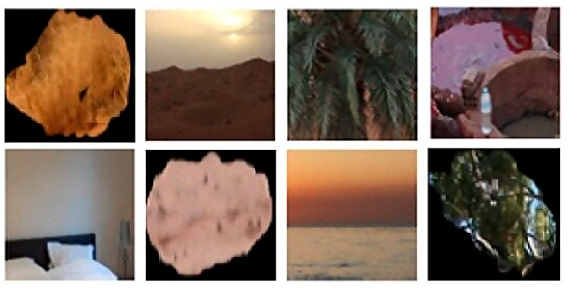
Figure 4. Random output samples show the true detection of the pristine image’s category. The output is flagged with the category name in green color “pristine” which indicates the correct decision.

In Figure 4, the model was able to justify the authenticity of these images and mark them as pristine images, which illustrates that the false positive is zero and the true positive is the one in the present experiment. On the other hand, in both Figure 5 and Figure 6 the model red flags these images as forged images regardless of whether the copy-move forgery type is active (as is in Figure 5) or passive (as is in Figure 6). These two cases are called true positive and true negative, respectively.

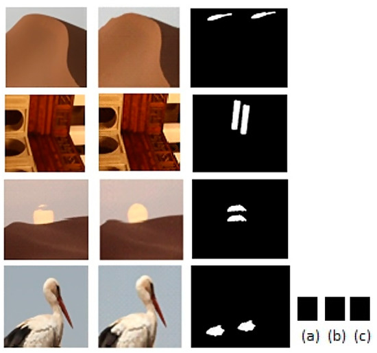
Figure 5. This figure presents three image categories (a) pristine image; (b) the same image was manipulated with copy-move forgery (c) the output mask showing the copy-move forgery detection result, including the two similar areas in the same image frame.

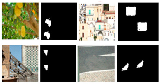
Figure 6. Random samples of the model result illustrate a true passive forgery detection i.e., there are no original images (pristine).

An unfortunate scenario occurs when the model marks the forged image as a pristine image. In this case, the model accuracy is reduced. However, even if a result mistakenly shows the image as pristine, the resulting flagging alarm may incorrectly act by sending the output category in red color as illustrated in Figure 7.

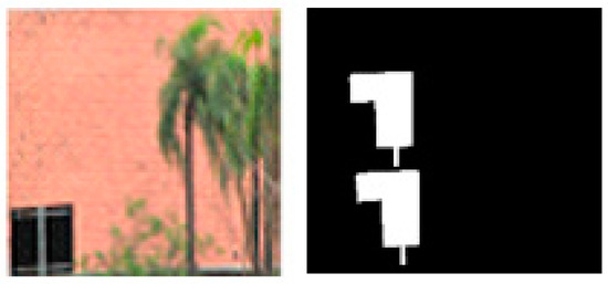
Figure 7. False detections by labeling this forged image as a pristine image. There will be a red flag in the results, referring to the false result.

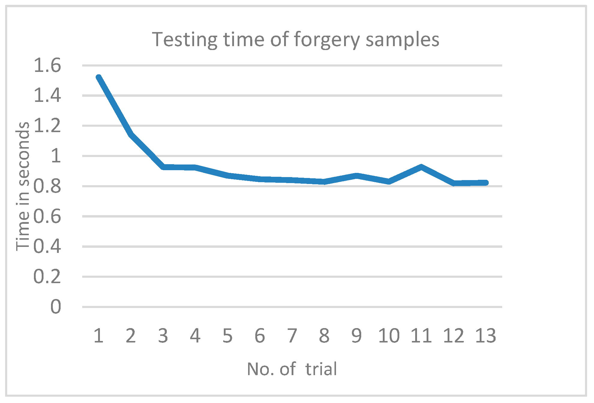
Our model represents a deep learning method suitable for detecting forgery embedded within digital images. Non-deep-learning traditional methods, such as [47], are unable to extract relevant data from input image patches automatically, nor can they devise representations very efficiently. Many non-deep-learning approaches also only utilize a single artificial feature for classification purposes. These are all significant drawbacks in the traditional models. Our proposed method, on the other hand, is much more efficient. It can apply several epochs in the training sets, the optimal number being no less than three epochs and no more than five, which is related to dataset size. Testing a new input image will take a longer time the first time round, but will decrease by several trials, the first of which usually takes no more than 1.6 s, as illustrated in Figure 8. This time is based on image resolution and the used machine. Table 4 indicates a clear reduction in accuracy from 90% to 81%. The average validation loss rate of the training set was around 0.3010 for all saturated iteration values. Of the 1255 forged images we used, we had an overall validation accuracy of 88.26% to 90.1%. The matrices and the baseline evaluation settings were devised by computing false positive (FP), true positive (TP), false positive (FP) and false negative (FN) settings in order to compute the F-measure. The evaluation scores in Table 5 present the F-measure of the proposed model vs. the state-of-the-art models [27,48,49]. It is worth mentioning again that our testing dataset was relatively small and used a mix of both forged and pristine images. Hence, we anticipate that the value will change in accordance with dataset size. Note that the number of epochs is low according to the dataset size to avoid overfitting during the training task.

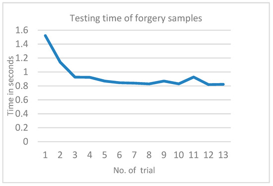
Figure 8. Testing time of forged samples related to the number the trials.

Table 4. The accuracy is based on the epoch and the number of the iterations.

Epoch	Iteration	Time Elapsed Sec.	Mini-batch Accuracy	Base Learning Rate
1	1	31.42	88.00%	0.0010
4	50	1587.43	90.00%	0.0010
7	90	3120.95	91.00%	0.0010

Table 5. Comparison of copy-move forgery detection F-measure, precision and recall of different algorithm.

Algorithm	[48]	[50]	[49]	[27]	[51]	[33]	Proposed
F1	0.5943	0.5439	0.6055	0.6318	0.7993	0.4926	0.8835
Precision	0.5440	0.5390	0.5662	0.5927	-	0.5734	0.6963
Recall	0.8020	0.8327	0.8040	0.8220	-	0.4939	0.8042

5. Conclusions

A novel neural network-based copy-move forgery detection strategy was proposed in this work. The convolutional neural network (CNN) was built with MATLAB due to its ease of use and its support of GPU/CPU (Computer Processing Unit) computations. Weights for decreasing error rates and improving overall efficiency were applied via backward and forward propagation. Our CNN learned how to reproduce both forged and pristine outputs in its training phase, enabling copied regions to trigger detection during reconstruction. The results of active copy-move detection were highly promising, while the passive detection results were only satisfactory. Additionally, overall efficiency was relatively low due to the small size of the experimental dataset utilized in the training phase. The proposed model’s key contribution is its capability of detecting and localizing copy-move forgery. In future related work, other network structures could be tested, and in-depth analyses could be performed through implementing a more expansive dataset than the one used here. Additionally, other kinds of image manipulation could be incorporated, including post-processing strategies. Futhermore, future work could focus on producing customized layers to distinguish the source and target location of the copy-moved region in this type of forgery, or to examine the effects of other shallow learning methods for image copy-move forgery.

References

- Jing, W.; Hongbin, Z. Exposing digital forgeries by detecting traces of image splicing. In Proceedings of the 8th IEEE International Conference on Signal Processing, Guilin, China, 16–20 November 2006; Volume 2. [Google Scholar]
- Christlein, V.; Riess, C.; Jordan, J.; Riess, C.; Angelopoulou, E. An evaluation of popular copy-move forgery detection approaches. IEEE Trans. Inf. Forensics Secur. 2012, 7, 1841–1854. [Google Scholar] [CrossRef]
- Ryu, S.J.; Kirchner, M.; Lee, M.J.; Lee, H.K. Rotation invariant localization of duplicated image regions based on Zernike moments. IEEE Trans. Inf. Forensics Secur. 2013, 1355–1370. [Google Scholar] [CrossRef]
- Li, H.; Luo, W.; Qiu, X.; Huang, J. IEEE Trans. Inf. Forensics Secur. 2017, 12, 1240–1252. [Google Scholar] [CrossRef]
- Korus, P.; Huang, J. Multi-scale analysis strategies in prnu-based tampering localization. IEEE Transl. Trans. Inf. Forensics Secur. 2017, 12, 809–824. [Google Scholar] [CrossRef]
- Lee, H.; Ekanadham, C.; Ng, A.Y. Sparse deep belief net model for visual area. In Advances in Neural Information Processing Systems; 20 (NIPS); MIT Press: Cambridge, MA, USA, 2008. [Google Scholar]
- Larochelle, H.; Bengio, Y.; Louradour, J.; Lamblin, P. Exploring strategies for training deep neural networks. J. Mach. Learn. Res. 2009, 10, 1–40. [Google Scholar]
- LeCun, Y.; Bottou, L.; Bengio, Y.; Haffner, P. Gradient-based learning applied to document recognition. Oroc. IEEE 1998, 2278–2324. [Google Scholar] [CrossRef]
- Giacinto, G.; Roli, F. Design of effective neural network ensembles for image classification purposes. Image Vis. Comput. 2001, 699–707. [Google Scholar] [CrossRef]
- Fukushima, K.; Miyake, S.; Ito, T. Neocognitron: A neural network model for a mechanism of visual pattern recognition. IEEE Trans. Syst. Man Cybern 1983, 826–834. [Google Scholar] [CrossRef]
- V, A.; L, K.; Gupta, A. Convolutional Neural Networks for Matlab. MatConvNet 2015, 1–59. [Google Scholar]
- He, K.; Zhang, X.; Ren, S.; Sun, J. Deep residual learning for image recognition. arXiv preprint 2015, arXiv:1512.03385. [Google Scholar]
- Verma, V.; Agarwal, N.; Khanna, N. DCT-domain Deep Convolutional Neural Networks for Multiple JPEG Compression Classification. Image Commun. 2017, 67, 1–12. [Google Scholar] [CrossRef]
- Krizhevsky, A.; Sutskever, I.; Hinton, G.E. Imagenet classification with deep convolutional neural networks. In Proceedings of the Advances in Neural Information Processing Systems, Lake Tahoe, NV, USA, 3–8 December 2012; pp. 1097–1105. [Google Scholar]
- Ren, S.; He, K.; Girshick, R.; Sun, J. Faster r-cnn: Towards real-time object detection with region proposal networks. In Proceedings of the Advances in Neural Information Processing Systems, Montreal, QC, Canada, 7–12 December 2015; pp. 91–99. [Google Scholar]
- He, K.; Zhang, X.; Ren, S.; Sun, J. Identity mappings in deep residual networks. arXiv preprint 2016, arXiv:1603.05027. [Google Scholar]
- Smeulders, A.W.; Worring, M.; Santini, S.; Gupta, A.; Jain, R. Content-based image retrieval at the end of the early years. IEEE Trans. Pattern Anal. Mach. Intell. 2000, 22, 1349–1380. [Google Scholar] [CrossRef]
- Voulodimos, A.; Doulamis, N.D.A.; Protopapadakis, E. Deep Learning for Computer Vision: A Brief Review. Hindawi. Comp. Intell. Neurosci. 2018, 1–13. [Google Scholar] [CrossRef] [PubMed]
- Yang, J.; Yu, K.; Gong, Y.; Huang, T. Linear spatial pyramid matching using sparse coding for image classification. In Proceedings of the IEEE Conference on Computer Vision and Pattern Recognition, Miami Beach, FL, USA, 20–25 June 2009; pp. 20–25. [Google Scholar]
- Felzenszwalb, P.F.; Girshick, R.B.; McAllester, D.; Ramanan, D. Object detection with discriminatively trained part-based models. IEEE Trans. Pattern Anal. Mach. Intell. 2010, 32, 1627–1645. [Google Scholar] [CrossRef] [PubMed]
- Jegou, H.; Perronnin, F.; Douze, M.; Sanchez, J.; Perez, P.; Schmid, C. Aggregating local image descriptors into compact codes. IEEE Trans. Pattern Anal. Mach. Intell. 2012, 34, 1704–1716. [Google Scholar] [CrossRef] [PubMed]
- Zeiler, M.D.; Fergus, R. Visualizing and understanding convolutional networks. In Proceedings of the European Conference on Computer Vision, Santiago, Chile, 11–18 December 2015; Springer: Berlin, Germany, 2015; pp. 818–833. [Google Scholar]
- Simonyan, K.; Zisserman, A. Very deep convolutional networks for large-scale image recognition. arXiv preprint 2015, arXiv:1409.155. [Google Scholar]
- Xie, S.; Girshick, R.; Dollar, P.; Tu, Z.; He, K. Aggregated residual transformations for deep neural networks. arXiv preprint 2016, arXiv:1611.05431. [Google Scholar]
- Das, S. CNNs Architectures: LeNet, AlexNet, VGG, GoogLeNet, ResNet and more. Available online: https://medium.com/analytics-vidhya/cnns-architectures-lenet-alexnet-vgg-googlenet-resnet-and-more-666091488df5 (accessed on 28 August 2017).
- Paulin, M.; Douze, M.; Harchaoui, Z.; Mairal, J.; Perronin, F.; Schmid, C. Local convolutional features with unsupervised training for image retrieval. In Proceedings of the IEEE International Conference on Computer Vision, Araucano Park, Las Condes, Chile, 11–18 December 2015; pp. 91–99. [Google Scholar]
- Liu, Y.; Guan, Q.; Zhao, X. Copy-move Forgery Detection based on Convoluational Kernel Network. Multimedia Tools Appl. 2018, 77, 18269–18293. [Google Scholar]
- Younis, A.; Iqbal, T.; Shehata, M. Copy-Move Forgery Detection Based on Enhanced Patch-Match. Int. J. Comput. Sci. Issues 2017, 14, 1–7. [Google Scholar]
- Soni, B.; Das, P.K.D.; Thounaojam, D. Cmfd: A detailed review of block based and key feature-based techniques in image copy-move forgery detection. IET Image Process. 2017. [Google Scholar] [CrossRef]
- Birajdar, G.K.; Mankar, V.H. Digital image forgery detection using passive niques. A survey. Digit. Investig. 2013, 10, 226–245. [Google Scholar] [CrossRef]
- Asghar, K.; Habib, Z.; Hussain, M. Copy-move and splicing image forgery detection and localization techniques. A review. Aust. J. Forensic Sci. 2017, 49, 281–307. [Google Scholar] [CrossRef]
- Radford, A.; Metz, L.; Chintala, S. Unsupervised Representation Learning with Deep Convolutional Generative Adversarial Networks. In Proceedings of the Computer Vision Conference ICLR, Caribe Hilton, San Juan, Puerto Rico, 2–4 May 2016; pp. 1–16. [Google Scholar]
- Wu, Y.; Abd-Almageed, W.; Natarajan, P. BusterNet: Detection Copy-Move Image Forgery with Source/Target Localization; Springer: Berlin, Germany, 2018. [Google Scholar]
- Huo, Y.; Zhu, X. High dynamic range image forensics using cnn. arXiv 2019, arXiv:1902.10938.2019. [Google Scholar]
- Isola, P.; Zhu, J.-Y.; Zhou, T.; Efros, A.A. Image-to-image translation with conditional adversarial networks. In Proceedings of the Conference on Computer Vision and Pattern Recognition, Honolulu, HI, USA, 21–26 July 2017. [Google Scholar]
- Bondi, L.; Baroffio, L.; Guera, D.; Bestagini, P.; Delp, E.J.; Tubaro, S. First Steps Toward Camera Model Identification with Convolutional Neural Networks. IEEE Signal. Process. Lett. 2017, 24, 259–263. [Google Scholar] [CrossRef]
- Sergey, I.; Szegedy, C. Batch normalization: Accelerating deep network training by reducing internal covariate shift. arXiv preprint 2015, arXiv:1502.03167. [Google Scholar]
- Yao, Y.; Shi, Y.; Weng, S.; Guan, B. Deep Learning for Detection of Object Forgery in Advanced video. Symmetry 2017, 3. [Google Scholar] [CrossRef]
- Mahendran, A.; Vedaldi, A. Visualizing deep convolutional neural networks using natural pre-images. Int. J. Comput. Vis. 2016, 12, 233–255. [Google Scholar] [CrossRef]
- Szegedy, C.; Liu, W.; Jia, Y.; Sermanet, P.; Reed, S.; Anguelov, D.; Erhan, D.; Vanhoucke, V.; Rabinovich, A. Going deeper with convolutions. In Proceedings of the IEEE Conference on Computer Vision and Pattern Recognition, Boston, MA, USA, 7–12 Jun 2015; pp. 1–9. [Google Scholar]
- Bayar, B.; Stamm, M.C. Design principles of convolutional neural networks for multi-media forensics. Soc. Imaging Sci. Technol. 2017, 10, 77–86. [Google Scholar]
- Ioffe, S.; Szegedy, C. Batch normalization: Accelerating deep network training by reducing internal covariate shift. In Proceedings of the 32nd International Conference on Machine Learning (ICML), Lille, France, 6–11 July 2015. [Google Scholar]
- Songtao, W.; Zhong, S.Z.; Yan, L. A novel convolutional neural network for image steganalysis with shared normalization. IEEE Trans. Multimed. 2017, 1–12. [Google Scholar] [CrossRef]
- Alex, K. Learning Multiple Layers of Features form Tiny Images; University of Toronto: Toronto, ON, Canada, 2009; pp. 1–58. [Google Scholar]
- James, P.; Relja, A.; Andrew, Z. Available online: http://robots.ox.ac.uk/~vgg/data/oxbuildings/ (accessed on 19 August 2019).
- Wen, B.; Zhu, Y.; Subramanian, R.; Ng, T.; Shen, X.; Winkler, S. COVERAGE—A Novel Database for Copy-Move Forgery Detection. In Proceedings of the IEEE International Conference Image Processing (ICIP), Quebec City, QC, Canada, 27–30 September 2015. [Google Scholar]
- Chen, S.; Tan, S.; Li, B.; Huang, J. Automatic Detection of Object-Based Forgery in Advanced Video. IEEE Trans. Circuits Syst. Video Technol. 2016, 26, 2138–2151. [Google Scholar] [CrossRef]
- Li, J.; Li, X.; Yang, B.; Sun, X. Segmentation-based image copy-move forgery detection scheme. Ieee Trans. Inf. Forensics Secur. 2015, 10, 507–518. [Google Scholar]
- Ulutas, G.; Muzaffer, G. A new copy move forgery detection method resistant to object removal with uniform background forgery. Hindawi Math. Probl. Eng. 2016, 1–19. [Google Scholar] [CrossRef]
- Silva, E.; Carvalho, T.; Ferreira, A.; Rocha, A. Going deeper into copy-move forgery detection: Exploring image telltales via multi-scale analysis and voting processes. J. Vis. Commun. Image Represent. 2015, 29, 16–32. [Google Scholar] [CrossRef]
- Ryn, S.J.; Lee, M.J.; Lee, H.K. Detection of copy-move forgery using Zernike moments. In Information hiding; Springer: Berlin, Germany, 2010; pp. 51–65. [Google Scholar]
© 2019 by the authors. Licensee MDPI, Basel, Switzerland. This article is an open access article distributed under the terms and conditions of the Creative Commons Attribution (CC BY) license (http://creativecommons.org/licenses/by/4.0/).