A Novel Orthogonal Extreme Learning Machine for Regression and Classification Problems

Abstract

An extreme learning machine (ELM) is an innovative algorithm for the single hidden layer feed-forward neural networks and, essentially, only exists to find the optimal output weight so as to minimize output error based on the least squares regression from the hidden layer to the output layer. With a focus on the output weight, we introduce the orthogonal constraint into the output weight matrix, and propose a novel orthogonal extreme learning machine (NOELM) based on the idea of optimization column by column whose main characteristic is that the optimization of complex output weight matrix is decomposed into optimizing the single column vector of the matrix. The complex orthogonal procrustes problem is transformed into simple least squares regression with an orthogonal constraint, which can preserve more information from ELM feature space to output subspace, these make NOELM more regression analysis and discrimination ability. Experiments show that NOELM has better performance in training time, testing time and accuracy than ELM and OELM.

1. Introduction

An extreme learning machine (ELM) is an innovative learning algorithm for the single hidden layer feed-forward neural networks (SLFNs for short), proposed by Huang et al [1], that is characterized by the internal parameters generated randomly without tuning. In essence, the ELM is a special artificial neural network model, whose input weights are generated randomly and fixed, so as to get the unique least-squares solution of the output weight [1], making the performance better [2,3,4]. In the conventional model there is a lack of convergence ability, generalization, over-fitting, local minimum and parameter adjustment, all of which make the ELM superior [1,5]. Considering the learning process of the ELM, it is relatively simple. Firstly, some internal parameters of the hidden layer are generated randomly, such as input weights connecting the input layer and hidden layer, the number of hidden layer neurons, etc., which are fixed during the whole process. Secondly, the non-linear mapping function is selected to map the inputting data to the feature space, and through analyzing the real output results and expected output results, the key parameter (output weight connecting the hidden layer and the output layer) can be directly obtained, omitting iterative tuning. So, its training speed is considerably faster than that of the conventional algorithms [6].

Due to the good performance of the ELM, it is used widely in regression and classification. For meeting higher requirements, researchers optimize and improve the ELM, and have proposed many better algorithms based on ELM. Di Wang et al. combined the local-weighted jackknife and RELM, proposed a novel conformal regressor (LW-JP-RELM), which complements ELM with interval predictions satisfying a given level of confidence [7]. For improving the generalization performance, Ying Yin et al. proposed enhancing the ELM by a Markov boundary-based feature selection, based on the feature interaction and the mutual information to reduce the number of features, so as to construct more compact network, whose generalization was improved greatly [8]. Ding et al. reformulated an optimization extreme learning machine to take a new regularization parameter, which is bounded between 0 and 1, and also easier to interpret as compared to the error penalty parameter $C$, it could achieve better generalization performance [9]. For solving sensibility of ELM to the ill-conditioned data, Hasan et al. proposed two novel algorithms based on ELM, ridge regression and almost unbiased ridge regression, and also gave three criteria to select the regularization parameter, which improved the generalization and stability of the ELM greatly [10]. Besides, there are more effective algorithms based on the ELM, such as Distributed Generalized Regularized ELM (DGR-ELM) [11], Self-Organizing Map ELM (SOM-ELM) [12], Data and Model Parallel ELM (DMP-ELM) [13], Genetic Algorithm ELM (GA-ELM) [14], Jaya optimization with mutation ELM (MJaya-ELM) [15], et al.

Either with a simple ELM or more complex algorithms based on ELM one must find the optimal solution of the two key parameters in ELM essentially, the number of hidden layer neurons and the output weights. From input layer to the output layer, essentially ELM learns the output weights based on the least squares regression analysis [16]. Therefore, many algorithms except those mentioned above are still proposed based on least squares regression, and their main work is to find an optimal transformation matrix, so as to minimize the error of sum-of-squares. Among these strategies [17,18], introducing orthogonal constraint into the optimization problem is required and also employed widely in the classification and subspace learning. Nie et al. showed that the performance of least squares discriminant and regression analysis after introducing orthogonal constraint is much better than those without orthogonal constraint [19,20]. After introducing orthogonal constraint into ELM, the optimization problem is seen as unbalanced procrustes problems, which is hard to be solved. Yong Peng et al. pointed out that the unbalanced procrustes problem can be transformed into a balanced procrustes problem, which is relatively simple [16]. Motivated by this research, in this paper we focus on the output weight, a novel orthogonal optimizing method (NOELM) is proposed to solve the unbalanced procrustes problem, and its main contribution is that the optimization of complex matrix is decomposed into optimizing the single column vector of the matrix, reducing the complexity of the algorithm.

The remainder of the paper is organized as follows. Section 2 reviews briefly the basic ELM model. In Section 3, the model formulation and the iterative optimization method are detailed. The convergence and complexity analysis is presented in Section 4. In Section 5, the experiments are conducted to show the performances of NOELM. Finally, Section 6 concludes the paper.

2. Extreme Learning Machine

Mathematically, given $N$ discrete sample ${\left(x_i, y_i\right)}_{i=1}^N$, where $N$ is the sample number, $x_i\in R^n$ is the input vector, $y_i\in R^m$ is the expected output vector, and the expected output of the $i\text{-}th$ sample is $y_i$, $y_i={\left[y_{i1} y_{i2} \dots y_{im} \right]}^T$, $i=1,2,3,\dots ,N$. 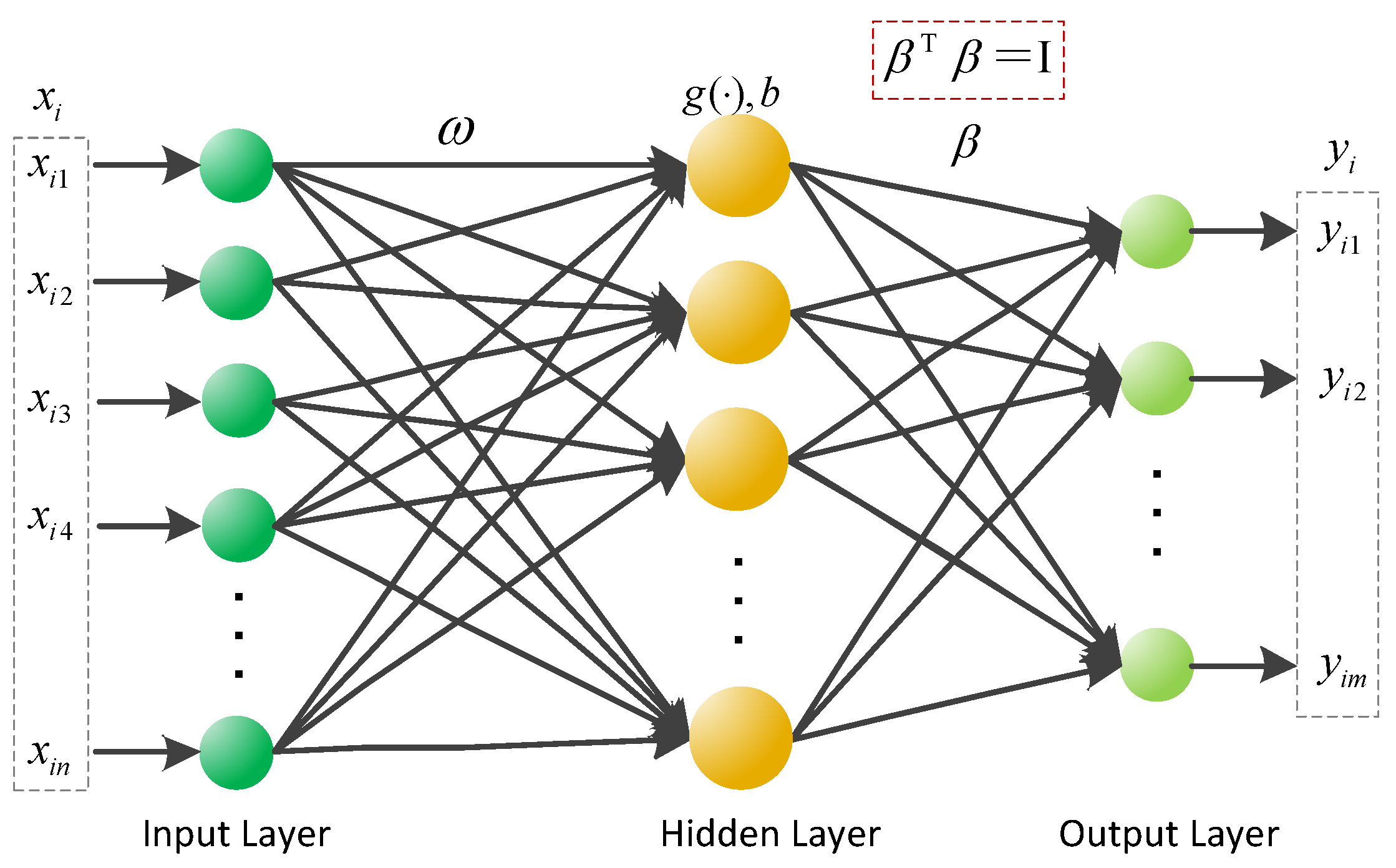For selected activation function, if the real output of the SLFNs is the same as the expected output $y_i$, the mathematical representation of SLFNs is as follows:

$$f\left(x_j\right)={\displaystyle \sum }_{i=1}^L{\beta }_i\mathrm{g}\left({\omega }_i,x_j,b_i\right)=y_j,$$

(1)

where ${\omega }_i={\left[{\omega }_{i1},\dots ,{\omega }_{in}\right]}^T$ is the input weight connecting the input layer to the $i\text{-}th$ hidden layer neuron, $b_i$ is the basis of the $i\text{-}th$ hidden layer neuron, ${\beta }_i={\left[{\beta }_{i1},\dots , {\beta }_{im}\right]}^T$ is the output weight connecting the $i\text{-}th$ hidden layer neuron and the output layer, and $L$ is the number of the hidden layer neurons, shown in Figure 1.

Equation (1) can be compactly rewritten as

$$H\beta =\mathrm{Y},$$

(2)

where

$$H={\left[\begin{array}{ccc}\mathrm{g}\left({\omega }_1,x_1,b_1\right)& \cdots & \mathrm{g}\left({\omega }_L,x_1,b_L\right)\\ ⋮& \ddots & ⋮\\ \mathrm{g}\left({\omega }_1,x_N,b_1\right)& \cdots & \mathrm{g}\left({\omega }_L,x_N,b_L\right)\end{array}\right]}_{N\times L},$$

(3)

$$\beta ={\left[\begin{array}{c}{\beta }_1^T\\ ⋮\\ {\beta }_L^T\end{array}\right]}_{L\times m},Y={\left[\begin{array}{c}{y}_1^T\\ ⋮\\ y_N^T\end{array}\right]}_{N\times m}.$$

(4)

So, based on the theory of ELM, the optimal solution of Equation (2) is as follows,

$$\beta =H^{†}\mathrm{Y},$$

(5)

where $H^{†}$ is the Moore–Penrose inverse of the Matrix $H$, $H^{†}= {\left(H^{T}H\right)}^{-1}{H}^T$. For further improving model precision, the regularization is introduced into ELM, the optimal problem is transformed as follows,

$$min: \frac{1}{2}\Vert H\beta -Y\Vert {}^2+\frac{C}{2}\Vert \beta \Vert {}^2,$$

(6)

where $C$ is the regularization parameter, which is used to balance the empirical risk and structural risk. Based on the Karush–Kuhn–Tucker condition, the optimal solution of $\beta$ is obtained:

$$\beta ={\left(H^{T}H+CI\right)}^{-1}{H}^{T}Y.$$

(7)

3. Novel Orthogonal Extreme Learning Machine (NOELM)

The orthogonal constraint is introduced into ELM, shown in Figure 1, the optimal problem is transformed as follows,

$$J\left({\beta }_{L+1}\right)=\underset{{\beta }_{L+1}^T{\beta }_{L+1}=I}{\min }\Vert H_{L+1}{\beta }_{L+1}-Y\Vert {}^2,$$

(8)

where $H_{L+1}\in R^{N\times \left(L+1\right)}$, ${\beta }_{L+1}\in R^{\left(L+1\right)\times m}$ is the output matrix and the output weight of the hidden layer, $Y\in R^{N*m}$. Because of the orthogonal constraint, the input samples are mapped into an orthogonal subspace, where their metric structure could be preserved.

Set $L>m$, so the problem (8) is an unbalanced orthogonal procrustes problem which is difficult to be resolved directly because of the orthogonal constraint [16]. In this paper, an improved method is proposed to optimize the problem (8) based on the following lemma.

Lemma 1

[[21], Theorem 3.1]. If ${\beta }_{L+1}^{*}=\left[{\rho }_1^{*},\dots ,{\rho }_{L+1}^{*}\right]$ is the optimal solution for the problem (8) and its orthogonal complement is $B_{L+1}^{*}$, then $H_{L+1}^T\left[Y, H_{L+1}^T{B}_{L+1}^{*}\right]$ is positive, semi-definite and symmetric, and

$$\Vert H_{L+1}^T{\rho }_j^{*}-y_j\Vert =\underset{{\rho }_j\perp {\tilde{\beta }}_j^{*},\Vert {\rho }_j\Vert {}^2=1}{\min }\Vert H_{L+1}{\rho }_j-{\widehat{y}}_j\Vert ,$$

(9)

where ${\tilde{\beta }}_j^{*}=\left[{\rho }_1^{*},\dots {\rho }_{j-1}^{*},{\rho }_{j+1}^{*},\dots ,{\rho }_{L+1}^{*}\right]$, ${\widehat{y}}_j$ is the $j\text{-}th$ column vector of $Y$.

The proof of Lemma 1 is simple, which can be found in the literature [21]. Motivated by Lemma 1, a local transformation is applied in the Equation (8), we relax the $j\text{-}th$ column ${\rho }_j$ ($j\le \left(L+1\right))$ and fix others, ${\tilde{\beta }}_j=\left[{\rho }_1,\dots ,{\rho }_{j-1},{\rho }_{j+1},\dots ,{\rho }_{L+1}\right]$, then the equation could be transformed into

$$J\left({\rho }_j\right)=\underset{{\rho }_j\perp {\tilde{\beta }}_j,\Vert {\rho }_j\Vert {}^2=1}{\min }\Vert H_{L+1}{\rho }_j-{\widehat{y}}_j\Vert {}^2.$$

(10)

If ${\rho }_j^{*}$ is the optimal solution of Equation (10), the approximation ${\beta }_{L+1}$ could be improved after replacing ${\rho }_j$ by ${\rho }_j^{*}$, and obviously, the modified ${\beta }_{L+1}^{*}=\left[{\rho }_1,\dots ,{\rho }_{j-1},{\rho }_j^{*},{\rho }_{j+1},\dots ,{\rho }_{L+1}\right]$ is also orthogonal.

To resolve the constrained problem (10) is a little difficult, so, the orthogonal complement $B_{L+1}$ of ${\beta }_{L+1}$ can be used to simplify the Equation (10). Set $P_{L+1}=\left[{\rho }_j,B_{L+1}\right]$, and it is known ${\rho }_j\perp {\tilde{\beta }}_j$, then $P_{L+1}$ is the orthogonal complement of ${\tilde{\beta }}_j$. So, in the constrained problem (10), the condition ${\rho }_j\perp {\tilde{\beta }}_j$ could be represented in another form, ${\rho }_j=P_{L+1}x$, $x\in R^{n-L}$ is a unit vector. Thus, the problem (10) can be transformed into the following form with quadratic equality constraint:

$$J\left(x\right)=\underset{x^2=1}{\min }\Vert H_{L+1}{P}_{L+1}x-{\widehat{y}}_j\Vert {}^2.$$

(11)

Clearly, after get the optimal solution $x^{*}$ of problem (11), the solution of problem (10) is ${\rho }_j=P_{L+1}{x}^{*}$. If the orthogonal complement of ${\beta }_{L+1}^{*}$ is $B_{L+1}^{*}$, then $B_{L+1}^{*}=P_{L+1}W$, $W$ is the orthogonal complement of $x^{*}$, and it can be constructed easily, using the Householder reflection $I-2u{\omega }^T$ with $\Vert \omega \Vert =1$, which meets $\left(I-2\omega {\omega }^T\right)x^{*}=-sign\left(x_1^{*}\right)e_1$, $x_1^{*}$ is the first component of $x^{*}$. Indeed, partitioning $P_{L+1}\left(I-2\omega {\omega }^T\right)$, ${\rho }_j^{*}$ and $B_{L+1}^{*}$ can be picked out from the following equation,

$$P_{L+1}\left(I-2\omega {\omega }^T\right)=\left[-sign\left(x_1^{*}\right){\rho }_j^{*}, B_{L+1}^{*}\right].$$

(12)

For resolving the problem (11), it first rewrites the Equation (11) in general form,

$$J\left(x\right)=\underset{{\Vert x\Vert }^2=1}{\min }\Vert Ax-y\Vert {}^2,$$

(13)

where $A=H_{L+1}{P}_{L+1}$, $y={\widehat{y}}_j$. $\Vert Ax-y{\Vert }^2$ is transformed in the following form

$$\begin{array}{ll}\hfill \Vert Ax-y{\Vert }^2=& \Vert Ax{\Vert }^2+\Vert y{\Vert }^2-2trace\left(x^T{A}^{T}y\right)\\ & \le \Vert A{\Vert }^2+\Vert y{\Vert }^2-2trace\left(x^T{A}^{T}y\right).\end{array}$$

(14)

Known from the Equations (13) and (14), the parameters $A$ and $y$ are fixed, the minimum problem of function $J\left(x\right)$ is transformed to the maximum of $trace\left(x^T{A}^{T}y\right)$ approximately, showing by Equation (15), denoted by $W=A^{T}y$.

$$x=\left\{X:X=\arg \max trace\left(X^{T}W\right)\right\}.$$

(15)

Let Singular Value Decomposition of $W$ be

$$W=Udiag\left({\Sigma }_k, O_{s-k}\right)V^T,$$

(16)

where $x\in R^{n-L}$, $s=n-L$, ${\mathsf{\Sigma }}_k=diag\left({\sigma }_1,\dots ,{\sigma }_k\right)$, ${\sigma }_1\ge {\sigma }_2\ge \dots \ge {\sigma }_k>0$, $k=rank\left(W\right)$, $U$ and $V$ are orthogonal.

Set $X^{*}=U^{T}XV$,

$$trace\left(X^{T}W\right)=trace\left(X^{*}diag\left({\Sigma }_k, O_{s-k}\right)\right).$$

(17)

So,

$$x=\left\{X:X=U{X}^{*}{V}^T,X=\mathit{arg}\mathit{max}trace\left(X^{*}diag\left({\Sigma }_k, O_{s-k}\right)\right)\right\},$$

(18)

As known above, $x\in R^{n-L}$ is a unit vector, partitioning $X^{*}$

$$X^{*}=\left[\begin{array}{c}{X}_{11}\\ X_{21}\end{array}\right],X_{11}\in R^k, X_{21}\in R^{\left(s-k\right)}.$$

(19)

Because of $x\in R^{n-L}$, then

$$\mathit{max}trace\left(X^{*}diag\left({\Sigma }_k, O_{s-k}\right)\right)=\mathit{max}trace\left(X_{11}^T{\Sigma }_k\right).$$

(20)

Note that $X^{*}=\left[x_{ij}\right]$ is unit and orthogonal, $\Vert X^{*}\Vert =1$, then $-1\le x_{ij}\le 1$, so based on the Equation (20), for the maximum, it can be deduced that $x_{ij}=1$, $i=j$, then $X_{11}=I_k$, $X_{21}\in O^{s-k}$, and $k=1$. Hence, $G\in O^{s-k}$,

$$x=\left\{X:X=U\left[\begin{array}{c}{I}_k\\ G\end{array}\right]V^T\right\}.$$

(21)

Based on the analysis above, the novel optimization to objective problem (8) is proposed in the position, its detail is as follows (Algorithm 1):

Algorithm 1: Optimization to objective problem (8)
Basic Information: training samples $\left\{{\left(x_i, y_i\right)}_{i=1}^N| x_i\in R^n, y_i\in R^m\right\}$
Initialization: Set threshold $\tau$ and $\eta$
S1.	Generate the input weight layer $w$ and bas vector $b$;
S2.	Calculate the output matrix of the hidden layer $H$ based on Equation (3);
S3.	Calculate the orthogonal ${\beta }^{\prime }$ of span $H^{T}Y$, and its orthogonal complement $B_{L+1}$, then $r_0=\Vert H{\beta }^{\prime }-Y\Vert$;
S3.	While$j=1,2,\dots ,m$
S4.	Relax the $j\text{-}th$ column ${\rho }_j$, ${\widehat{y}}_j$ from the matrix $\beta$, $Y$ separately, and fix the rest;
S5.	Set $P=\left[{\rho }_j,B_{L+1}\right]$, then solve $x=\arg \underset{\Vert x\Vert =1}{\min }\Vert HPx-{\widehat{y}}_j{\Vert }^2$;
S6.	Set $A=HP$, $y={\widehat{y}}_j$, then $W=A^{T}y$. By SVD, $W=Udia\left({\mathsf{\Sigma }}_k, O_{s-k}\right)V^T$, so as to obtain $U$ and $V$;
S7.	Based on the Equation (21), $x=U{I}_k{V}^T$;
S8.	Calculate the vector $u=\left(x+s{e}_1\right)/\Vert x+s{e}_1\Vert$, $s=sign\left(x\right)$;
S9.	Partition $P\left(I-2u{u}^T\right)=\left[-s{\rho }_j^{*},B_{L+1}^{*}\right]$ so as to obtain ${\rho }_j^{*}$ and $B_{L+1}$, then replace ${\rho }_j$ of $\beta by {\rho }_j^{*}$ to obtain ${\beta }^{*}$, $B_{L+1}=B_{L+1}^{*}$ and $\beta ={\beta }^{*}$;
	End While
S10.	Calculate $r_1=\Vert H{\beta }^{*}-Y\Vert$, then if $\left(r_0-r_1\right)<\tau r_1\parallel r_1\le \eta$, terminate, otherwise, $r_0=r_1$, $B_{L+1}$ is the new orthogonal complement of ${\beta }^{*}$, go to step S3.

4. Convergence and Complexity Analysis

Considering the convergence if the algorithm, Let $\left\{{\beta }^{i, j}\right\}$ be a sequence of ${\beta }^{*}$ generating during iteration, which converges to $\beta$, so, its orthogonal complement $B^{i, j}$ also converges to $B$, where $i$ is the iterating number, and $i$ is the operation of relaxing the $j\text{-}th$ column from original matrix, so, it follows $P^{i,j}=\left[{\rho }_j^{i,j}, B^{i, j}\right]$ converges to $P=\left[{\rho }_j, B\right]$.

Based on the equations above, it is know that ${\rho }_j^{*}$ is the optimal solution of Equation (10). If $\Vert H{\rho }_j-{\widehat{y}}_j\Vert -\Vert H{\rho }_j^{*}-{\widehat{y}}_j\Vert =\eta$, then for $i$ is large enough, $P^{i,j}$ and $P$ meets

$$\Vert P^{i,j}-P\Vert =\Vert \left[{\rho }_j^{i,j}, B^{i, j}\right]-\left[{\rho }_j, B\right]\Vert <\frac{\eta }{4\Vert H{\Vert }_2},$$

(22)

Set ${\rho }_j^{*}=Px$, $\Vert x\Vert =1$, and ${\widehat{\rho }}_j=P^{i,j}x$, then based on Equation (22), it has

$$\Vert {\widehat{\rho }}_j-{\rho }_j^{*}\Vert =\Vert P^{i,j}x-Px\Vert \le \Vert P^{i,j}-P\Vert \Vert x\Vert <\frac{\eta }{4\Vert H{\Vert }_2},$$

(23)

Based on Equations (10) and (22), it has

$$\Vert {\widehat{\rho }}_j-{\rho }_j^{*}\Vert =\Vert P^{i,j}x-Px\Vert \le \Vert P^{i,j}-P\Vert \Vert x\Vert <\frac{\eta }{4\Vert H{\Vert }_2},$$

(24)

Based on the Equations (23) and (24), it has

$$\begin{array}{cc}\hfill f\left({\beta }^{i,j}\right)-f\left({\beta }^{i+1,j}\right)& =\Vert H{\beta }^{i,j}-Y\Vert -\Vert H{\beta }^{i+1,j}-Y\Vert \hfill \\ & =\Vert H{\rho }_j^{i,j}-{\widehat{y}}_j\Vert -\underset{\rho \perp {\tilde{\beta }}_j^{i+1,j},\Vert \rho \Vert =1}{\min }\Vert H\rho -{\widehat{y}}_j\Vert \hfill \\ & \ge \Vert H{\rho }_j^{i,j}-{\widehat{y}}_j\Vert -\Vert H{\widehat{\rho }}_j-{\widehat{y}}_j\Vert \hfill \\ & \ge \Vert \left(H{\rho }_j-{\widehat{y}}_j\right)+H\left({\rho }_j^{i,j}-{\rho }_j\right)\Vert +\Vert \left(H{\rho }_j^{*}-{\widehat{y}}_j\right)+H\left({\widehat{\rho }}_j-{\rho }_j^{*}\right)\Vert \hfill \\ & \ge \Vert \left(H{\rho }_j-{\widehat{y}}_j\right)\Vert -\Vert H\left({\rho }_j^{i,j}-{\rho }_j\right)\Vert -\Vert \left(H{\rho }_j^{*}-{\widehat{y}}_j\right)\Vert -\Vert H\left({\widehat{\rho }}_j-{\rho }_j^{*}\right)\Vert \hfill \\ & \ge \Vert \left(H{\rho }_j-{\widehat{y}}_j\right)\Vert -\Vert \left(H{\rho }_j^{*}-{\widehat{y}}_j\right)\Vert -\Vert H\left({\rho }_j^{i,j}-{\rho }_j\right)\Vert -\Vert H\left({\widehat{\rho }}_j-{\rho }_j^{*}\right)\Vert \hfill \\ & \ge \eta -\frac{\eta }{4}-\frac{\eta }{4}\hfill \\ & \ge \frac{\eta }{2}\hfill \end{array}$$

So, $f\left({\beta }^{i,j}\right)-f\left({\beta }^{i+1,j}\right)\ge \frac{\eta }{2}$, based on the derivation of the inequality above, it can deduced that $f\left({\beta }^{1,j}\right)>f\left({\beta }^{2,j}\right)>\dots >f\left({\beta }^{n,j}\right)$. By the same method and analysis, it also can be obtained that $f\left({\beta }^{i,1}\right)>f\left({\beta }^{i,2}\right)>\dots >\left({\beta }^{i,m}\right)$. So, it is $f\left({\beta }^{1,1}\right)>f\left({\beta }^{1,2}\right)>\dots >f\left({\beta }^{2,1}\right)>\dots >f\left({\beta }^{3,1}\right)>\dots$, so the sequence $\left\{f\left({\beta }^{i,j}\right)\right\}$ is monotonically decreasing, and when $i\to \infty$, $f\left({\beta }^{i,j}\right)-f\left({\beta }^{i+1,j}\right)\to 0$. In a word, after analysis above, the novel algorithm monotonically decreases the objective shown in Equation (8).

It is known that the complexity of ELM derives from the calculation of output weights $\beta$, or rather, it is mainly used to calculate the inverse of matrix $H^{T}H+CI$. In most cases, the number of hidden layer neurons $L$ is much smaller than the training sample size $N$, $L\ll N$, thus the complexity is less than least square support vector machine (LS-SVM) and proximal support vector machine (PSVM), which need to calculate the inverse of $N\times N$ matrix [16]. As we know, the complexity of ELM and OELM is $O\left(L^3\right)$, $O\left(t\left(N{L}^2+L^3\right)\right)$ separately. As for the complexity of the novel algorithm proposed in the paper, its main calculation is from the loop. In each iteration, $\mathrm{it}\mathrm{needs}\mathrm{to}\mathrm{find}\mathrm{the}\mathrm{optimal}\mathrm{solution}\mathrm{of}\mathrm{one}\mathrm{column}$ relaxing from $\beta$, and during this, it needs to do SVD decomposition on the $m\times 1$ matrix $A^{T}y$, whose complexity is $O\left(m^2\right)$, and then, the complexity of updating $\beta$ once is $O\left(m\right)$. So, the complexity of the proposed algorithm is $O\left(t{m}^3\right)$, where $t$ is the number of updating $\beta$. In real application, regardless of classification or regression, the output dimension is much less than the number of hidden layer neurons and the training samples size.

As we know, ${\left(H\beta \right)}^T=Y^T$, then ${\beta }^T{h}_i^T\left(x_i\right)=y_i$. Considering the Euclidean distance between any two data points $y_i$ and $y_j$, because of the orthogonal constraint ${\beta }^T\beta =I$, it has $\Vert y_i-y_j\Vert =\Vert h_i\left(x_i\right)-h_j\left(x_j\right)\Vert$. It is known that $h_i\left(x_i\right)$ is the point in the ELM feature space, $\Vert h_i\left(x_i\right)-h_j\left(x_j\right)\Vert$ is the distance in ELM space, and $\Vert y_i-y_j\Vert$ is the distance in the subspace. From this analysis, the novel ELM with orthogonal constraints is superior in maintaining the metric structure from first to last.

5. Performance Evaluation

For testing the performances of the novel algorithm proposed in the paper, it is compared with other learning algorithms on the classification problems (EMG for Gestures, Avila and Ultrasonic Flowmeter) and regression problems (Auto price, Breast cancer, Buston housing, etc.), which are from the University of California Irvine (UCI) machine learning repository [22], shown in

Table 1. The specification of the datasets.

Datasets	Training	Testing	Attributes	Class
Avila	5000	2000	10	12
Electro-Myo-Graphic data (EMG) for Gestures	10000	2000	6	8
Ultrasonic Flowmeter	112	69	33	4
Stock	450	500	9	-
Abalone	2000	1177	8	-
Auto price	80	79	14	-
Auto-Miles Per Gallon (MPG)	320	78	8	-
Breast cancer	100	94	32	-
Buston housing	250	256	13	-
California housing	8000	12640	8	-
Census house (8L)	10000	12784	8	-

. These learning algorithms include ELM [1], OELM [16] and I-ELM [23,24], their activation function is the sigmoid function, and the number of hidden layer neurons is set as three times as the input dimension. For I-ELM, the initial number of hidden layer neurons is set to zero. In the real experiments, the key parameters such as the input weights, the biases, etc., are generated randomly from $\left[-1,1\right]$, and then, all samples are normalized into $\left[-1,1\right]$, and the outputs of the regression problems are normalized into $\left[0,1\right]$ [25]. All simulations are done in Matlab R2016a environment.

In the classification problems, ELM and OELM are selected to compare with NOELM. The experimental results are shown in Figure 2 and Figure 3. Figure 2 shows the convergence property of NOELM. At first, the convergence rate is larger, the objective value falls rapidly, when reaching about 0.8, it falls slowly, until stable. During the whole process, the number of iterations does not vary significantly, the maximum is not more than 20, and the minimum is only about 5, so in a word, the novel algorithm is a little more effective. Figure 3 shows the comparison of the training time and classification rate. Due to the complexity above, the traditional ELM is low in complexity, and its training time is shortest. The complexity of NOELM is less than OELM, then its training time is shorter than OELM, and longer than that of ELM because of too many iterations, but the difference is not larger than 0.05. Although NOELM is not the best in terms of training time, its classification is better than the other two, the largest rate can reach 0.9.

In the regression problems, ELM, OELM and I_ELM are selected to compare with NOELM, the experimental results are shown in

Table 2. Comparison of the network complexity and training time.

	ELM		OELM		I_ELM		NOELM
	Nodes	Time(s)	Nodes	Time(s)	Nodes	Time(s)	Nodes	Time(s)
Auto price	42	0.0325	42	0.0677	50	0.0374	42	0.0241
Breast cancer	96	1.0217	96	2.1285	66	0.2324	96	0.7568
Buston housing	39	0.0453	39	0.0944	100	0.5672	39	0.0336
Auto-MPG	24	0.8835	24	1.8406	76	0.8173	24	0.6544
Stock	27	0.6392	27	1.3317	97	0.8039	27	0.4735
Abalone	24	0.4836	24	1.0075	40	0.3237	24	0.3582
California housing	24	0.4547	24	0.9473	69	6.0856	24	0.3368
Census house (8L)	24	0.7667	24	1.5973	57	5.2479	24	0.5679

. As mentioned above, the number of hidden layer neurons is determined based on the input dimension, so the hidden layer neurons of ELM, OELM and NOELM are fixed, and the others are dynamically increasing hidden layer neurons. Analyzing the information of Table 2, compared with I_ELM, the network complexity of NOELM is a little lower, and its structure is more compact, but it is a little worse than I_ELM in some datasets, the difference is not large and fully acceptable. As for the accuracy of training and testing from

Table 3. Comparison of the average of training and testing (Root Mean Square Error).

	ELM		OELM		I_ELM		NOELM
	Train	Test	Train	Test	Train	Test	Train	Test
Auto price	0.1283	0.1297	0.1141	0.1212	0.0997	0.1089	0.1056	0.1161
Breast cancer	0.13182	0.1499	0.1163	0.1340	0.1132	0.1219	0.1070	0.1245
Buston housing	0.1695	0.1708	0.14122	0.1502	0.1403	0.1353	0.1243	0.1379
Auto-MPG	0.1513	0.1584	0.1291	0.1394	0.1321	0.1363	0.1159	0.1279
Stock	0.1380	0.1423	0.1195	0.1245	0.1197	0.1227	0.1084	0.1138
Abalone	0.1327	0.1339	0.1171	0.1179	0.1109	0.1125	0.1077	0.1082
California housing	0.2555	0.2574	0.2265	0.2280	0.1993	0.2035	0.2092	0.2103
Census house (8L)	0.1439	0.1489	0.1254	0.1286	0.1017	0.1023	0.1143	0.1164

and

Table 4. Comparison of the standard deviation of training and testing (Root Mean Square Error).

	ELM		OELM		I_ELM		NOELM
	Train	Test	Train	Test	Train	Test	Train	Test
Auto price	0.0033	0.0234	0.0024	0.0215	0.0031	0.0196	0.0018	0.0204
Breast cancer	0.0099	0.0209	0.0088	0.0188	0.0085	0.0167	0.0082	0.0176
Buston housing	0.0130	0.0183	0.0085	0.0148	0.0126	0.0135	0.0059	0.0126
Auto-MPG	0.0142	0.0179	0.0101	0.0141	0.0134	0.0162	0.0077	0.0118
Stock	0.0161	0.0172	0.0125	0.0131	0.0147	0.0158	0.0103	0.0106
Abalone	0.0058	0.0066	0.0053	0.0059	0.0049	0.0056	0.0050	0.0054
California housing	0.0047	0.0061	0.0068	0.0082	0.0027	0.0038	0.0080	0.0094
Census house (8L)	0.0034	0.0038	0.0026	0.0043	0.0006	0.0028	0.0033	0.0046

, comparing with ELM and OELM, the performances of NOELM is better, it has better stability. Because of characteristics of I_ELM, it constructs a more compact network and is a little superior in the training and testing accuracy in some datasets, and this is just the weak point of NOELM and other related algorithms. However, by introducing the orthogonal constraints and improving the algorithm, NOELM can greatly narrow this gap, and its performance is also acceptable.

6. Conclusions

In this paper, referring to the idea of OELM, the orthogonal constraint is introduced into the ELM, then a novel orthogonal ELM is proposed (NOELM), which is a special supervised learning algorithm theoretically. By contrast with the OELM, the main characteristic and contribution is to transform the complex unbalanced orthogonal procrustes problem to a simple least squares problem with orthogonal constraint based on the single vector, and to optimize the single column vector of the output weight matrix so as to obtain the optimal solution of the whole matrix. Compared with ELM and OELM, NOELM can achieve a much better neural network at fast convergence rate and higher training and testing accuracy. Although NOELM is a little weaker than I_ELM in some aspects, the gap is very narrow, and the result is still acceptable.