Abstract
In a real manufacturing environment, the set of tasks that should be scheduled is changing over the time, which means that scheduling problems are dynamic. Also, in order to adapt the manufacturing systems with fluctuations, such as machine failure and create bottleneck machines, various flexibilities are considered in this system. For the first time, in this research, we consider the operational flexibility and flexibility due to Parallel Machines (PM) with non-uniform speed in Dynamic Job Shop (DJS) and in the field of Flexible Dynamic Job-Shop with Parallel Machines (FDJSPM) model. After modeling the problem, an algorithm based on the principles of Genetic Algorithm (GA) with dynamic two-dimensional chromosomes is proposed. The results of proposed algorithm and comparison with meta-heuristic data in the literature indicate the improvement of solutions by 1.34 percent for different dimensions of the problem.
1. Introduction
Scheduling (assigning resources to tasks) is one of the most important decisions in the optimal utilization of facilities and equipment. Research in this area can be divided into two parts—static environments and dynamic environments. Most of the methods discussed in the literature can solve the static scheduling but do not consider dynamic events, such as different times of new orders, staff reductions, and machine failure. In the scheduling problems, if the set of tasks don’t change over time, then the manufacturing system is static. In contrast, if new a task is added to the set of tasks during the time, this system is a dynamic manufacturing system [1,2]. In other words, in a dynamic manufacturing system, all tasks are available (at zero time) simultaneously. But, in an actual Sequence of operations, the runtime of tasks needs to be considered. In practice, scheduling problems are dynamic and the main reason for that is that some of the mentioned parameters change over the time. Therefore, the dynamic nature of a scheduling problem should be considered to solve practical problems [3,4]. It has been proved that solving static models is easier than dynamic models and wide reviews have been done on them [5].
Current research, consider the flexibility of operation and flexibility due to parallel machines in addition to considering the dynamic manufacturing environment (due to the non-zero entry time of tasks to the workshop).
In general, in classic manufacturing models, there is only one processing route for each task, which leads to the lack of flexibility in such production systems. In such environments, production flexibility is a key competitive weapon, and having this capability becomes a competitive advantage that causes to able them to quickly respond to unpredictable changes.
For example, having some flexibility in an industrial production context for powerful manufacturing systems leads to being adaptable to fluctuations, such as machine failure and bottlenecking of machine creation. And then each machine can produce several products [6,7].
Today, most manufacturing systems keep several versions of each machine at each workstation (flexibility due to parallel machines) to solve the bottleneck problem (due to long processing times for some components or due to machine failure) and to increase production and improve performance. Some operations can be processed not only on one station but also on a set of stations available in the workshop (flexibility due to operation). These conditions add another complexity to this problem, so finding an approximately optimal solution for these problems is very complicated and difficult [8,9,10,11,12].
In the literature, these problems are known as flexible scheduling problems. In a comprehensive survey that was conducted in 2000, the dimensions of this flexibility were expanded to 15 [13].
In this paper, Flexible Dynamic Job-Shop with Parallel Machines (FDJSPM) in manufacturing environments has been studied. There are n components and m workstations in which each component needs a certain set of operations (O) and the sequence of movement between workstations is different for each component. In this study, we consider a dynamic workshop in order to be more relevant for actual manufacturing environments. Each component enters the workshop at time r (a random and non-zero time). To avoid bottlenecks and increase production rates, each workstation can process more than one component (due to operation flexibility). Each workstation M includes L parallel machines with non-uniform speeds and can process the assigned tasks (because of the flexibility of parallel machines with uniform speeds).
The aim of this paper is to model the problem and then solve the problem of minimizing the workflow by considering the dynamics generated in the workshop, i.e., operation flexibility and the flexibility of the parallel machines with non-uniform speed. In this study, for the first time, we consider the operational flexibility and the flexibility due to parallel machines with non-uniform speed for a dynamic job shop.
Accordingly, the FDJSPM problem splits into two subproblems: allocation and sequencing of operations. The allocation subproblem is caused by the flexibility generated in job-shop production, and increases the complexity of the problem.
This paper consists of 7 sections. The introduction and research necessity are investigated in this section. The literature on the subject and related work in the field of flexible, dynamic, and static manufacturing systems are presented in Section 2. The problem definition and the mathematical model are introduced in Section 3. The proposed approach is defined in Section 4. Numerical experiments and experimental results are presented in Section 5 and Section 6, respectively. Results of the research and future work are presented in Section 7. The following, literature review and research background in the field of “job-shop”, “flexible job-shop” and “scheduling by parallel machines with uniform and non-uniform speeds” are presented.
2. Related Work
Classic Job-Shop Scheduling (JS) and Dynamic Job-Shop Scheduling (DJS) are the most important production management problems and one of the most difficult combinatorial optimization problems. Generally, research done on scheduling in dynamic environments has been based on either queuing theory or rolling time horizon. In the first case, the scheduling problem is considered as a queuing system and new orders go on devices after arrival and they are processed based on their prioritization.
Analytical methods for solving this problem are based on queuing theory [1]. Due to the complexity of the problem, the above-mentioned analytical methods can solve the problems with one machine. The rolling time horizon technique is an efficient way to provide schedules for dynamic problems in which the dynamic scheduling problem is split into several static scheduling problems and in each stage, each problem is solved statically. This method was applied to solve medium-term scheduling problems [1]. Then, it was used to investigate the scheduling problem and significant results were presented in this field [14]. Later, researchers used general solutions to use this method in backward scheduling [15]. Recently, scheduling problems in dynamic and uncertain environments have been investigated by using RTH methods and their performances evaluated in different situations.
In the JS problem, the route of tasks is fixed and it isn’t necessary to have the same route for all tasks. In this problem, we assume that there is one processing route for each task, which leads to the lack of flexibility in manufacturing systems.
Flexible Job Shop Scheduling (FJS) is an extension of JS, in which each operation can be processed by a set of machines. According to the definition, FJS includes two subproblems: routing (assign the machine to the operation) and scheduling (sequencing the operations) [16].
FJSPM is an extension of FJS and parallel machines. In each step of FJS, there is only one machine. In FJSPM, there is more than one machine at least in one step, and in each step, a set of parallel machines are placed together and each of them can process the operation assigned to that step. Thus, we can choose a different route to process the operations. In fact, a new kind of flexibility is defined for JS which has not been considered in the literature. The main idea of this flexibility is to increase the production, address the bottleneck problem, and use it as a competitive advantage in the economic environment.
In 1998 [17], mixed three-stage JS with a particular structure; one machine in step 1 and 3 and two machines in step 2, was investigated with the aim of minimizing the maximum completion time . In the same year, a Taboo Search Algorithm (TS) was also presented for FJSPM in order to reduce the [18].
In 1999 [19] a study proposed a multi-objective algorithm to solve the flexible process. They formulated the machine loading problem as a two-criteria integer program and proposed two different meta-heuristic models, one of which is based on theory and the other is based on the GA. In the same year, a hybrid genetic-based algorithm was proposed to minimize the in FJS [20]. After that, in 2001, a polynomial algorithm with/without considering interruption was proposed for FJS [21]. In 2002, for the first time, FJS was investigated in a multi-purpose case [22], and the proposed algorithm was a hybrid of fuzzy logic and evolutionary algorithms. The flexibility of the problem was limited only to the operational flexibility. Fuzzy logic is used to search the target space in order to find the Pareto solutions.
In the same year, a GA was proposed for the same FJS problem in the supply chain to reduce the [23]. They assume the existence of external sources, machine replacement for each operation, and sequences of multiple operations for each component.
In 2003 [24], a symbiotic evolutionary algorithm (an evolutionary algorithm) which is based on artificial intelligence was proposed. Some researchers tried to solve the FJS problem by using heuristic methods and fuzzy logic [25]. In 2004, the flexibility in JS was limited to the operation flexibility [26]. The aim of this research was to reduce the latency and TS was used to solve the problem. In 2004, a GA was proposed for the problem that researchers had discussed in 2002 [27]. In this study, at first, the allocation subproblem is solved by the priority rule SPT and then, based on the most important step of finding the best answer (selecting an appropriate representation of the chromosomes step), a GA with chromosome representation based on the base operations is proposed. Computational results show the effectiveness of the algorithm in dealing with large problems.
The simulated annealing algorithm (SA) is proposed for Multi-Stage Job Shop with Parallel Machines (MSJSPM) with the aim of minimizing the total current time [28]. Also, problems studied in previous years [22] were investigated in this year [29] and a hybrid hierarchy method was proposed for that problem. In this method, Particle Swarm Optimization (PSO) is used for solving the routing subproblem, and SA is used for solving the sequence of operations. In 2004, a new method was proposed for economic scheduling of multi-products with a general cycle in FJS [30] and a multi-objective and efficient practical hierarchy method was proposed for FJS [31]. This method is a hybrid of PSO and SA. Then, a new algorithm based on the Artificial Immune System (AIS) for FJS with turning back was proposed [32].
In 2006, FJS with uniform parallel machines, with the aim of minimizing the , was studied [33]. They developed a set of meta-heuristic algorithms and showed that for a large number of tasks, a vector addition based meta-heuristic is optimal. Researchers used three kinds of flexibility; totally (FJSP-100), average (FJSP-50), and partial (FJSP-20) [3]. They said that C% flexibility means all operations of different tasks can be processed by C% of available machines in JS [1]. In 2007, overreliance of evolutionary algorithms on recombination mechanisms and random selection was the most important limitation of evolutionary algorithms [34].
In order to overcome these limitations and obtain efficient solutions for FJSP, they tried to take advantage of the interaction between learning and evolution, and then they presented their GA, named Hybrid Genetic Algorithm (HGA). Their algorithm was a hybrid of the evolutionary algorithm, learning pattern, and population generation. A simple distribution rule used for population generation and K-nearest neighborhood were used for the learning pattern. A combination of the Bottleneck transmission method and a GA was used for FJS with three objectives in 2007 [35]. They utilized the chromosome display method in [27] which uses 2 vectors instead of 1 vector for machine assignment and sequence of operations. Also, they utilized the global search capability of GA and the local search capability of the Bottleneck transmission method to solve the problem. In [30,31], the authors examined scheduling in flexible flow lines with sequence-dependent setup times to minimize the makespan. This type of manufacturing environment is found in industries, such as printed circuit board and automobile manufacture. An integer program that incorporates these aspects of the problem is formulated and discussed. Because of the difficulty in solving the IP directly, several heuristics are developed, based on greedy methods, flow line methods, the Insertion Heuristic for the Traveling Salesman Problem (TSP), and the Random Keys GA.
Generally, the results of a comprehensive study on the fields of “job shop”, “flexible job shop”, and “job-shop scheduling with uniform/non-uniform parallel machine”, show that in most sequences, all tasks are assumed to be available simultaneously. But, in real manufacturing environments, the set of tasks which must be scheduled vary over time. This fact shows the dynamicity of the job-shop problem. In addition, being adaptable to fluctuations, such as machine failure and bottlenecks of machine creation, is very important for such systems.
These adaptations are generated by considering base flexibilities. In such a way, manufacturing systems could use them as competitive advantages in addition to overcoming such fluctuations. Therefore, by reviewing the literature and identify existing gaps, we investigate the FDJSPM.
For the first time, in this research, we consider “operational flexibility” and “flexibility due to parallel machines with non-uniform speed” in the field of the dynamic JS model. In the following, we model the problem with the aim of minimizing the flow time (Fmax).
3. Problem Definition and Mathematical Model
In this section, we will present the variables and introduce the FDJSPM problem, then present an integer programming model, and finally prove the NP-hard feature of the problem.
3.1. Problem Definition
The FDJSPM problem is defined as follow: there are m processing steps (workstations) for n tasks (component) in JS where each task needs a set of operations. The Ith component enters the dynamic job-shop at a non-zero time (ri). The Jth component consists of a chain of operations, which, without losing the generality, we can assume is the same as the order of processing tasks in JS. The order of movement between workstations is different for various tasks (the main feature of manufacturing tasks). The number of operations needed for task completion is smaller or equal to the number of processing steps. In each step of processing, Mk, we need lk versions of parallel machines with various speeds. Each of them can process the assigned operations to that step. In a flexible workstation, this parameter (lk) is larger than 1. Each operation can be processed by at least one workstation, and because of the operational flexibility, there is at least one operation which can be processed on more than on a workstation.
The time needed to process the operation Oi,j on a machine with Sk,pm = 1 in the kth step is equal to Ppm,j,k, if this operation is processed on a machine with Sk,pm > 1 the time may be reduced to . The aim of this paper is to reduce the maximum flow time of components .
According to the definition, the FDJSPM problem is decomposed into two sub-problems: assignment subproblem (assign tasks to flexible workstations) and sequencing operations (Sequencing operations among the tasks in the waiting queue of each workstation). The assignment subproblem is further decomposed into two subproblems: workstation assignment and machine assignment. The assignment subproblem is caused by the operational flexibility and parallel machines in JS which increase the complexity of the problem. The aim of this paper is to minimize the by considering the following assumptions:
- At a given time, each machine can process only one operation.
- JS is dynamic and tasks enter to JS at a non-zero time.
- At a given time, each task can be processed by only on one machine.
- All machines are available at time 0 and never break down.
- Interrupting the operation is not allowed and the processing time of each task is definite and known.
- Available depot is allowed and its capacity is infinite.
- Preparation time between operations is negligible. It’s either a part of the processing time or the transportation time and can be ignored.
Some of the above assumptions are unrealistic in practice and are considered for simplifying the model.
3.2. Sets, Parameters, and Variables Definition
- n: The number of entered tasks to the JS at the non-zero time
- ni: The number of operations of ith component
- ri: Entered the time of ith component to the JS
- m: The number of processing steps (workstations)
- k: Index of steps (workstations) k = 1, …, m
- Mk: kth step of processing
- Mk,r: rth parallel machine of kth step
- Oi,j: ith operation of jth task
- Sti,j: Step in which operation oi,j will be processed
- lk: The number of parallel machines in kth step
- lmax: Maximum of lk
- pm: Index of parallel machines in workstations; pm=1, …, lk
- Sk,r: Speed of Mk,r
- Pi,j: Time units to process the operation oi,j on a machine with unit speed
- A: An optional big number
- Fmax: Maximum flow time
- ci,j: Earliest finish time of oi,j
- : Finish time of oi,j on machine Mk,pm
If machines in kth step are possible machines for oi,j, this variable is 1, otherwise, it is 0.
If oi,j be processed on machine Mk,pm this variable is 1, otherwise, it is 0.
If op,q be processed before oi,j on Mk,pm this variable is 1, otherwise it is 0.
3.3. Mathematical Models
3.3.1. Objective Function
Minimization of flow time
3.3.2. Constraints of the Problem
3.4. Model Description
In order for scheduling to be feasible, it’s necessary to assign each operation to the right recourses [1]. Equation (2) ensures that operations don’t have any interference. In other words, these Equations lead to process operations in an appropriate order.
Since two operations cannot be processed on one machine at the same time, a valid schedule must consider resource limitations to solve the problem [1]. Equations (3) and (4) ensure that operations on one processor don’t have interference.
All models presented for JS have at least 2 similar limitations. All JS problems have constraints 1, 2, and 3 in common. The innovation of this paper is as follows:
- (a)
- Equations (5) and (6) ensure each operation of each task is assigned to one machine. In other words, Equation (5) ensures that each task must be processed only on one machine and be processed just one time. These equations are generated due to the flexibility of parallel machines in workstations. Beside these equations, Equation (7) explain that if in step K, Oi,j isn’t assigned to each machine, its completion time on all machines must be 0. These equations are generated due to the flexibility considered in JS.
- (b)
- On the other hand, because the objective function is based on the completion (finish) time, Equation (8) computes the maximum finish time. Equation (9) is considered to study the dynamic property of the problem due to differences in the arrival time of jobs in the workshop.
We used lingo software to evaluate the proposed model and we solved the small and average FDJSPM problem with this model. The results confirm the validity of the proposed model to solve the FDJSPM problem.
3.5. NP-Hard Problem
The complexity of a combinatorial problem is the amount of time spent to solve that problem. The FDJSPM problem is an extension of the FDJSP problem but with flexibility due to parallel machines in a dynamic manufacturing environment. So, its complexity and hardness are the same as for the FDJSP problem. If operational flexibility is considered in these problems, the complexity of finding the optimal approximate solutions is increased [1]. Since FDJSP with operational flexibility is strongly NP-hard [8], this problem, with respect to parallel machines in a dynamic manufacturing environment, will also be strongly NP-hard.
3.6. Problem-Solving Approach
For solving such scheduling problems, we need an efficient method. This method must be able to consider the complexities arising from the exponential increase in the solution space to find a proper solution.
In this paper, we utilize the capability of a GA to design an efficient method to solve the problem. In the following section, the structure of the proposed GA for solving the FDJSPM problem is introduced and then parameters and the efficiency of the proposed algorithm based on numerical experiments are shown.
4. The Proposed Algorithm
Since the FDJSPM problem is categorized as a NP-hard problem, there is no algorithm to find an efficient solution in a reasonable time for large or medium size problems. If an algorithm is able to find a proper solution, it needs a long time. In this section, a GA is proposed which is able to find a solution in a reasonable time. Figure 1 shows the general procedure of the proposed GA.
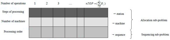
Figure 1.
Chromosome representation in the proposed genetic algorithm (GA).
The main components of GA are: chromosome representation, initial population generation, fitness function, crossover and mutation operator, and selection method. The parameters of the GA, including the population size, number of generations, probability of crossover (pc), and probability of mutation (pm), must be predefined [22].
4.1. Chromosome Representation (Problem Encoding)
The first step in JS or any optimization problem using GA is to represent the solutions in the form of chromosomes [36].
One of the capabilities of using the GA is to design the solutions corresponding to chromosomes (schedules). If chromosome design and classic operations are applied efficiently, one can avoid generating inefficient chromosomes, and it is not necessary to use the penalty or repairing strategy. In the literature on the use of genetic algorithms to solve problems, many criteria have been defined to design chromosomes. Among them, criteria such as least amount of space and time due to the computational complexity of the problem also avoid generating inefficient chromosomes [1].
The FDJSPM problem is decomposed to two subproblems: “allocation” and “sequencing the operations”. The proposed GA is designed in such a way that it is able to solve these two sub-problems seamlessly and simultaneously.
For this purpose, a two-dimensional dynamic chromosome with respect to the dynamicity of entering tasks to the system is presented (Figure 1). In this representation, chromosome length is equal to all the operations for scheduling (nTOP) and its width is equal to 3. So, each solution is presented as a two-dimensional array.
This method is similar to the method used in 2002, in which the allocation sub-problem was decomposed into two distinct sub-problems: workstation allocation and machine allocation.
In this representation, the first row of the chromosome shows the workstation processing the desired operation and the second row is the number of the machine that will process this operation. The third row contains the priority assigned to each operation. Each element in the third row is always a number between 1 and nTOP and the priority of two chromosomes cannot be the same. Thus, the obtained solution is always justified. In general, we can say that the first two rows indicate the allocation and the third row indicates the sequence of operations.
In order to understand the encoding system, consider an example containing 4 jobs and 3 workstations. A flexible manufacturing system with parallel machines is designed in such a way that each job has 3 operations and each workstation has 3, 2, 2 uniform parallel machines, respectively. Also, the manufacturing system is completely flexible. The chromosome corresponding to the solution contains 3 rows of length 12 and is encoded as in Figure 1. Chromosome representation is as follow:
The sequence is based on field operations, and the processing operation is the first of a string assigned to Station.
According to Figure 1 and Figure 2, it is clear that each chromosome is logically divided into several parts. The number of segments of each chromosome is equal to the number of jobs. Plans for subdivisions of each job are in the same range and in the first row. In the next row of chromosomes, the overall arrangement of chromosomes is determined.
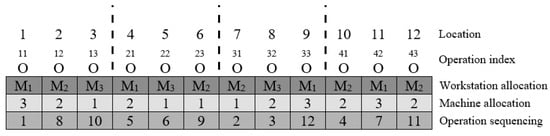
Figure 2.
Chromosome representation according to the obtained solution.
In this way, various mutation and crossover operators can be designed. Separating different aspects of the scheduling will make searching in solution space easier.
4.2. Initial Population
After determining the method of converting solutions to chromosomes, an initial chromosome must be produced. How to produce the initial population is a key step in determining the quality of the solutions in any local search method, such as a GA. Random generation of the initial population results in retention of the diversity of chromosomes in the initial population, reduces the possibility of premature convergence, and falls in local optima [35].
In the proposed GA, in order to avoid premature convergence, no heuristic method is used to produce the initial population. Thus, rows 1 and 2 are filled out by allocating a flexible workstation randomly and row 3 is filled out with a random combination of numbers 1 to nTOP.
4.3. Crossover Operation
The proposed GA uses two positions based on crossover and RMX crossover with the rate of Pc. Position-based crossover can be applied to the machine allocation row (rows 1 and 2 of the chromosome) and RMX crossover can be applied to the sequence of operations (row 3 of the chromosome). In position-based crossover, some genes are selected randomly from the first parent (P1) and are exactly copied in the child chromosome (O1). To complete the remaining genes, we use the second parent (P2) and copy the non-repetitive genes to the same positions in O1.
RMX crossover is applied on the sequence of operations (row 3 of chromosomes). This method was proposed by Goldberg and Langley. In fact, it is the same as 2-point crossover in the literature which is extended for special cases. In this method, two chromosomes P1 and P2 must be cut at a random position. This position is called the “mapping point”. Genes between these two mapping points are exchanged between P1 and P2. Now, to create the third row of O1, we must permutate the genes of P1 and P2 in O1 and O2 until there is no inconsistency in terms of non-identical sequence numbers. These genes are obtained by one-to-one correspondence obtained from the exchange of genes between the two cut points.
4.4. Mutation Operation
In general, mutation not only creates unplanned random changes, but also provides a wider search space and can prevent premature convergence. For this reason, in the proposed algorithm, the permutation operation is applied to each parent chromosome separately after applying the crossover operation. In this manner, for each element of a string, the possibility of mutation is tested. If this test is successful, that chromosome will be mutated.
In the proposed GA, because of the special structure of the problem and the proposed chromosome, a heuristic mutation operation based on linear inversion (a heuristic rule) is proposed. This operation works with two different mutation rates. So, for allocation, the sub-problem uses heuristic mutation with rate , and for the sequencing operation, the sub-problem uses linear inversion with rate . In this manner, if the testing result on a chromosome is positive, a gene from that chromosome is selected randomly and its workstation allocation field is changed to another number, which represents a flexible workstation.
To better understand the mutation operator, an example is given in this section. The chromosome selected for mutation is the chromosome of Figure 2. In this chromosome, the machine allocation and operational sequencing rows are mutated. It is assumed that O32 is mutated on the basis of the probability of mutation and further, based on the probability of the mutation , the order of execution is completely changed. The result of the jump operator is shown in Figure 3. The mutated sections are underlined.
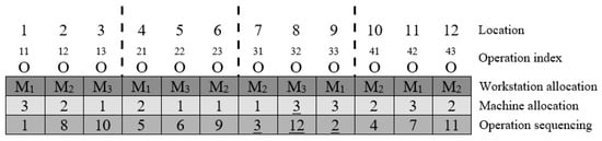
Figure 3.
Mutation example.
4.5. Selection Method
The proposed GA uses developed sampling space. This space is defined as follow: if the initial population size is α and after applying crossover and mutation operations β children are produced, the sampling spec size will be . The sampling method to produce the next generation will be elitism and the rolled-wheel selection method.
We use the elitism method to produce good solutions and increase the chance of achieving the optimal solution [28]. Based on the elitism method, a number of chromosomes are selected and transferred to the next generation without any preconditions.
If the values of consecutive chromosomes are equal, these chromosomes aren’t selected, and the next chromosomes will be tested. In GA, the numbers of the best chromosomes of each generation are placed directly in the next generation. The aims of this method are:
- (1)
- In general, some chromosomes in each generation have the highest degree of fitness. These chromosomes have the best genes and, due to having the best fitness, can produce better chromosomes for subsequent generations.
- (2)
- This method increases the likelihood of the best parents moving to the next generation.
4.6. Fitness Function
The fitness function computes the effectiveness of selected solutions or created schedules. Our aim is to reduce the maximum flow time (Fmax), so a low fitness is assigned to solutions which have the highest Fmax. Here, the fitness function of the ith chromosome is and Fmax(i) is the maximum flow time in chromosome ith.
An example of editing the response sequence is shown in Figure 4 for calculating fitness.
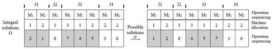
Figure 4.
How to edit the sequence of operations.
4.7. Strategy for Dealing with Restrictions
The other issue in the GA is to deal with problem’s restrictions, because genetic operators used in the algorithm may generate unjustified chromosomes. There is a corrective strategy in our algorithm to deal with these restrictions. In this strategy, an unjustified chromosome is transformed to a justified chromosome instead of being removed (Figure 3).
4.8. Termination of Genetic Algorithm
The algorithm of Figure 5 will terminate after max-gen repetitions.
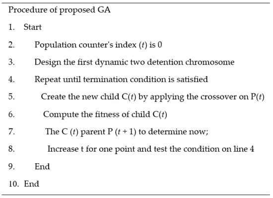
Figure 5.
Procedure of the proposed genetic algorithm.
5. Numerical Experiments
5.1. Comparison Method
Since the FDJSPM problem has not yet been considered, there is no similar algorithm to compare the proposed method with. So, in order to show the superiority of the proposed algorithm, we use the Random Keys Genetic Algorithm (RKGA) algorithm which was proposed in 2004 for the FSPM problem [37,38]. RKGA is a meta-heuristic algorithm which is designed for the FSPM problem with flexibility due to parallel machines with uniform speeds and the flexibility of operations in workstations. For this reason, the problem solved by this algorithm has the highest similarity to the FDJSPM problem. We can use it easily and without losing the generality. So, we consider the JSPM problem as a special case of the FDJSPM problem.
The developers of the RKGA algorithm used a hierarchical approach to solve their problem and decompose their problem into two sub-problems; allocation (task allocation to flexible workstations) and sequencing (sequence of processing). they then decomposed the allocation sub-problem into two sub-problems: workstation allocation and machine allocation. The allocation sub-problem is generated because of the flexibility of operations and parallel machines.
In studies conducted in 2004, for task scheduling, the RKGA method was used in the first step and then SPT Cyclic Heuristic (SPTCH) contributions and the Johnson rule were used for assigning tasks to machines in such a way that each task was allocated to a machine which can process the allocated task at the earliest time. In fact, in this algorithm, the first tasks are scheduled by RKGA, and then contributions are used to schedule the following operations [38]. We also use this equivalent concept for the FDJSPM problem. It means that the first operations of tasks are scheduled by RKGA and the following contributions are used to schedule the later operations [39].
5.2. Generate Random Problems
To generate random problems, 6 parameters are identified as Table 1. For the first five parameters, the RKGA algorithm is used [37,38] and U (1, 3) is considered as the processing speed of machines.

Table 1.
Level of agents to perform the GA.
In general, all combinations of this level will be tested. Some other restrictions are introduced below. For machine distribution agents, it is necessary that at least one machine stage is different from the others. Also, the maximum number of machines in a stage must be lower than the number of tasks. At least one stage must have a number of parallel machines larger than 1. So, with 10 machines at each stage and 6 jobs removed, 6 compound machines and 6 jobs can be added at any stage. Ten datasets for each test scenario were generated.
5.3. Design of Experiments
Algorithms (both proposed algorithm and RKGA algorithm) are coded in C++ language and were run on a computer with a Pentium IV CPU, 3 GHz, and 1GB of RAM and in Borland C++ 5.02. Each algorithm (proposed GA and RKGA) runs with 720 sets of information.
5.4. Setting Parameters
Different parameter values have a significant impact on the quality of the obtained solutions by the GA.
Here we only use the parameter setting procedure to set three parameters . For this purpose, one set is selected from each scenario (there are 10 data sets in each scenario). In total, 72 datasets are selected randomly, and then in the parameter setting procedure, the GA will be run on 72 datasets by creating new parameters. The average fitness is calculated for each run. First, we consider the following parameter values:
The percent of selection of the best chromosome for the next generation : 5%, 10%, 15%, 20%, 25%.
Probability of crossover : 0.3, 0.4, 0.5, 0.6, 0.7, 0.8, 0.9
Probability of mutation : 0.005, 0.01, 0.015, 0.02, 0.025
Number of initial population (pop-size): 100
Number of generations (Max-gen): 125
In the parameter setting procedure, at first, we change the value of one parameter in its defined domain, then fix the other parameters in their minimum value, and finally define the best for the changeable parameter based on their fitness, and then we change the other parameter in the next stage by fixing this value for the mentioned parameter. Of course, in addition to these fixed parameters, other parameters are kept at their minimum values and, as for the previous stage, the best value is selected for changeable parameters. This procedure is repeated until all parameters are fixed. Computational results show the best-obtained values for as 20%, 0.7 and 0.02 respectively. (Table 2).
Table 2.
Values of GA parameters after setting.
6. Computational Results
In this section, the performance of the proposed GA algorithm for the FDJSPM problem with the aim of reducing the maximum flow time will be compared to RKGA. The comparison was performed for 216 scenarios and was run 10 times as shown in Table 3.
Table 3.
Comparison of the proposed GA and the RKGA.
A main index named “the average minimization of the maximum flow time of tasks” is used to compare these methods and other auxiliary indexes, such as “the minimum value of minimization of the maximum flow time of tasks during different runs”, “average time to solve each scenario”, and “the fold improvement in objective function” and different size of problem (small, medium, and large) are used. The results of this comparison, according to Table 4 and Table 5, are as follow:
Table 4.
Average solving time of the proposed GA and RKGA.
Table 5.
Improvement and percent of improvement between the proposed GA and RKGA.
- According to the “the minimum value of the minimization of the maximum flow time of tasks” index, and for 10 runs of each of the 72 scenarios of different sizes (small, medium, large), the proposed GA has an average improvement of 0.57%, 1.02%, and 1.17%, and an overall improvement of 0.92% above RKGA.
- “Average objective function” for 10 runs on 72 datasets seems the best criterion for evaluating these algorithms. As seen in Table 3, according to this criterion for small, medium, and large size problems, the proposed algorithm has 1.17%, 1.35%, and 1.49% average improvement and an overall improvement of 1.34% higher than RKGA.
- According to the “improvement of objective function” index for small, medium, and large size problems, the proposed algorithm has 50, 46.7, and 52-fold improvement, respectively, and on average has a 49.6-foldimprovement over RKGA.
- According to “average objective function” index for small, medium, and large size problems, the proposed algorithm has an average improvement of 40, 42, and 49-fold from 72 runs, respectively, and, overall, has an average improvement of 49.6% above RKGA.
- According to “average time for solving the problem”, the proposed algorithm has no significant improvement for small problems, but for medium and large problems, it has an average increase of 14.5% and 33.8%, respectively, and has worse performance than RKGA.
“Average difference between GA and RKGA” is a suitable criterion to show the performance of the proposed algorithm. For this index, there are 1.17%, 1.35%, and 1.49% improvements (for small, medium, and large problems) for the proposed algorithm. This result shows with increasing the size of the problem, the proposed algorithm has greater improvement than RKGA.
Finally, the results show that the proposed GA requires more time to solve the problem, but with respect to the improvements obtained from minimum and average on the objective function, this increased time is justified. Therefore, according to the numerical results, the effectiveness of the proposed algorithm against the RKGA is confirmed.
Figure 6 shows the Average Fmax comparison for the two algorithms.
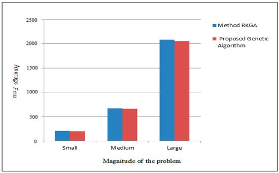
Figure 6.
Average Fmax Comparison.
Investigating the results obtained from the proposed algorithm and comparing it with the RKGA method shows that the proposed method is slightly better than the previous one. For big problems, this gap is slightly higher. The main reason for this result is the use of intelligent intersection operators and mutants that can search the response space more effectively than RKGA.
7. Conclusions
In this paper, the flexible job-shop scheduling problem with parallel machines (with non-uniform speed) in each workstation for dynamic manufacturing systems (because time entrance of tasks is variable) is introduced. Then, a mixed integer nonlinear programming model is presented. Then, Fmax as an objective function is investigated, with the aim of the efficient utilization of machines by reducing the time that recourses are used for, thus increasing the rate and speed of the manufacturing process, which is the most important goal in the manufacturing supply chain. We utilize the capability of a GA to solve the time and scheduling problems. Due to the dynamicity of manufacturing, dynamic two-dimensional chromosomes are provided. Chromosomes and genetic operators are designed in such a way that there is minimal dealing with constraints and unjustified chromosomes. In the proposed GA, the initial population is generated randomly and doesn’t have any information about the problem. This maintains the diversity of the population and reduces the possibility of premature convergence. Also, the influence of strong chromosomes is reduced and premature convergence to the local optimum is avoided by preventing the entrance of duplicate chromosomes into the next generation. After setting our proposed genetic parameters, its performance was compared to the RKGA method and it was observed that our genetic algorithm requires more time to solve the problem than the RKGA method. However, this time allows improvements in the minimum and average value of the objective function. Computational results show improvements of 1.17%, 1.35% and 1.49, and 1.34% on average, for small, medium, and large problems. Thus, according to the numerical experiments, the efficiency of the proposed algorithm is confirmed as greater than for RKGA. Increasing the efficiency of proposed algorithm and reducing the execution time are considered as future goals. On the other hand, in actual manufacturing issues, decision makers are often faced with multiple objectives. Selecting the right combination of objectives and investigating the problem in a multi-objective case and in a stochastic environment is essential. As future work, our algorithm could be integrated with other methods. For example, using a local search algorithm can improve the performance of the GA.
Author Contributions
A.K.S. has conceived, designed and formulated the complete paper; M.Y.S. and M.S. helped to design the algorithms; S.M.B. and A.A.R.H. have investigated data analytics and formulated the methodology of a paper; J.W. improved the algorithms, performance analysis and results.
Acknowledgments
This work is supported by the National Natural Science Foundation of China (61772454, 61811530332, 61811540410, U1836208).
Conflicts of Interest
The authors declare no conflict of interest.
References
- Baker, K.R. Introduction to Sequencing and Scheduling; John Wiley & Sons: New York, NY, USA, 1974. [Google Scholar]
- Hosseinabadi, A.R.; Siar, H.; Shamshirband, S.; Shojafar, M.; Nasir, M.H.N.M. Using the gravitational emulation local search algorithm to solve the multi-objective flexible dynamic job shop scheduling problem in Small and Medium Enterprises. Ann. Oper. Res. 2015, 229, 451–474. [Google Scholar] [CrossRef]
- Tay, J.C.; Ho, N.B. Evolving dispatching rules using genetic programming for solving multi-objective flexible job-shop problems. Comput. Ind. Eng. 2007, 54, 453–473. [Google Scholar] [CrossRef]
- Shamshirband, S.; Shojafar, M.; Hosseinabadi, A.R.; Kardgar, M.; Nasir, M.H.; Ahmad, R. OSGA: Genetic-based open-shop scheduling with consideration of machine maintenance in small and medium enterprises. Ann. Oper. Res. 2015, 229, 743–758. [Google Scholar] [CrossRef]
- Farahabadi, A.B.; Hosseinabadi, A.R. Present a New Hybrid Algorithm Scheduling Flexible Manufacturing System Consideration Cost Maintenance. Int. J. Sci. Eng. Res. 2013, 4, 1870–1875. [Google Scholar]
- Hosseinabadi, A.R.; Farahabadi, A.B.; Rostami, M.S.; Lateran, A.F. Presentation of a New and Beneficial Method Through Problem Solving Timing of Open Shop by Random Algorithm Gravitational Emulation Local Search. Int. J. Comput. Sci. 2013, 10, 745–752. [Google Scholar]
- Shojafar, M.; Kardgar, M.; Hosseinabadi, A.R.; Shamshirband, S.; Abraham, A. TETS: A Genetic-based Scheduler in Cloud Computing to Decrease Energy and Makespan. In Proceedings of the 15th International Conference on Hybrid Intelligent Systems (HIS 2015), Seoul, Korea, 16–18 November 2015; Chapter Advances in Intelligent Systems and Computing. Volume 420, pp. 103–115. [Google Scholar]
- Gena, M.; Zhang, W.; Line, L.; Yun, Y.S. Recent advances in hybrid evolutionary algorithms for multiobjective manufacturing scheduling. Comput. Ind. Eng. 2017, 112, 616–633. [Google Scholar] [CrossRef]
- Wang, J.; Ju, C.; Gao, Y.; Sangaiah, A.K.; Kim, G. A PSO based Energy Efficient Coverage Control Algorithm for Wireless Sensor Networks. Comput. Mater. Contin. 2018, 56, 433–446. [Google Scholar]
- Tirkolaee, E.B.; Hosseinabadi, A.R.; Soltani, M.; Sangaiah, A.K.; Wang, J. A Hybrid Genetic Algorithm for Multi-trip Green Capacitated Arc Routing Problem in the Scope of Urban Services. Sustainability 2018, 10, 1366. [Google Scholar] [CrossRef]
- Chen, J.C.; Wub, C.C.; Chen, C.W.; Chen, K.H. Flexible job shop scheduling with parallel machines using Genetic Algorithm and Grouping Genetic Algorithm. Expert Syst. Appl. 2012, 39, 10016–10021. [Google Scholar] [CrossRef]
- Dalfard, V.M.; Mohammadib, G. Two meta-heuristic algorithms for solving multi-objective flexible job-shop scheduling with parallel machine and maintenance constraints. Comput. Math. Appl. 2012, 64, 2111–2117. [Google Scholar] [CrossRef]
- Vokurka, R.J.; O’Leary-Kelly, S.W. A review of empirical research on manufacturing exibility. J. Oper. Manag. 2000, 18, 85–501. [Google Scholar] [CrossRef]
- Naderi, B.; Azab, A. Modeling and heuristics for scheduling of distributed job shops. Expert Syst. Appl. 2014, 41, 7754–7763. [Google Scholar] [CrossRef]
- Shahrabi, J.; Adibi, M.A.; Mahootchi, M. A reinforcement learning approach to parameter estimation in dynamic job shop scheduling. Comput. Ind. Eng. 2017, 110, 75–82. [Google Scholar] [CrossRef]
- Yazdani, M.; Aleti, A.; Khalili, S.M.; Jolai, F. Optimizing the sum of maximum earliness and tardiness of the job shop scheduling problem. Comput. Ind. Eng. 2017, 107, 12–24. [Google Scholar] [CrossRef]
- Riane, F.; Artiba, A.; Elmaghraby, S.E. A hybrid three-stage flowshop problem: Efficient heuristics to minimize makespan. Eur. J. Oper. Res. 1998, 109, 321–329. [Google Scholar] [CrossRef]
- Nowicki, E.; Smutniciki, C. The flow shop with parallel machines: A taboo search approach. Eur. J. Oper. Res. 1998, 106, 226–253. [Google Scholar] [CrossRef]
- Brandimarte, P. Theory and methodology, exploiting process plan flexibility in production scheduling: A multi-objective approach. Eur. J. Oper. Res. 1999, 114, 59–71. [Google Scholar] [CrossRef]
- Ghedjati, F. Genetic algorithms for the job-shop scheduling problem with unrelated parallel constraints: Heuristic mixing method machines and precedence. Comput. Ind. Eng. 1999, 37, 39–42. [Google Scholar] [CrossRef]
- Jansen, K. Approximation algorithms for flexible job shop problems. Int. J. Found. Comput. Sci. 2001, 12, 521–534. [Google Scholar]
- Kacem, I.; Hammadi, S.; Borne, P. Approach by localization and multi objective evolutionary optimization for flexible job-shop scheduling problems. IEEE Trans. Syst. Man Cybern. 2002, 32, 1–13. [Google Scholar] [CrossRef]
- Lee, Y.H.; Jeong, C.S.; Moon, C. Advanced planning and scheduling with outsourcing in manufacturing supply chain. Comput. Ind. Eng. 2002, 43, 351–374. [Google Scholar] [CrossRef]
- Kim, Y.K.; Park, K.; Ko, J. A symbiotic evolutionary algorithm for the integration of process planning and job shop scheduling. Comput. Oper. Res. 2004, 30, 1151–1171. [Google Scholar] [CrossRef]
- Allet, S. Handling flexibility in a “generalised job shop” with a fuzzy approach. Eur. J. Oper. Res. 2003, 147, 312–333. [Google Scholar] [CrossRef]
- Scrich, C.A.; Armentano, V.A.; Laguna, M. Tardiness minimization in a flexible job shop: A taboo search approach. J. Intell. Manuf. 2004, 15, 103–115. [Google Scholar] [CrossRef]
- Gen, M.; Cheng, R. Genetic Algorithm in Search, Optimization and Machine Learning; Addition-Wesley: Reading, MA, USA, 2004; ISBN 0201157675. [Google Scholar]
- Low, C. Simulated annealing heuristic for flow shop scheduling problem with unrelated parallel machines. Comput. Oper. Res. 2005, 32, 2013–2025. [Google Scholar] [CrossRef]
- Xia, W.; Wu, Z. An effective hybrid optimization approach for multi-objective flexible job-shop scheduling problems. Comput. Ind. Eng. 2005, 48, 409–425. [Google Scholar] [CrossRef]
- Torabi, S.A.; Karimi, B.; Fatemi-Ghomi, S.M.T. The common cycle economic lot scheduling in flexible job shops: The finite horizon case. Int. J. Prod. Econ. 2005, 97, 52–65. [Google Scholar] [CrossRef]
- Wang, J.X.X. Complexity and algorithms for two-stage flexible flow shop scheduling with availability constraints. Comput. Math. Appl. 2005, 50, 1629–1638. [Google Scholar]
- Tay, J.C.; Wibowo, D. An effective chromosome representation for evolving flexible job-shop scheduling. In Proceedings of the Genetic and Evolutionary Computation Conference (GECCO), Seattle, WA, USA, 26–30 June 2004; pp. 210–221. [Google Scholar]
- Kyparisis, G.J.; Koulamas, C. Flexible flow shop scheduling with uniform parallel machines. Eur. J. Oper. Res. 2004, 168, 985–997. [Google Scholar] [CrossRef]
- Ho, N.B.; Tay, J.C.; Lai, E. An effective architecture for learning and evolving flexible job shap schedules. Eur. J. Oper. Res. 2007, 179, 316–333. [Google Scholar] [CrossRef]
- Gao, J.; Gen, M.; Sun, L. Scheduling jobs and maintenances in flexible job shop with a hybrid genetic algorithm. J. Intell. Manuf. 2007, 17, 493–507. [Google Scholar] [CrossRef]
- Park, B.J.; Choi, H.R.; Kim, H.S. A hybrid genetic algorithm for the job shop scheduling problems. Comput. Ind. Eng. 2003, 45, 597–613. [Google Scholar] [CrossRef]
- Kurz, M.E.; Askin, R.G. Scheduling flexible flowlines with sequence-dependent setup times. Eur. J. Oper. Res. 2004, 159, 66–82. [Google Scholar] [CrossRef]
- Kurz, M.E.; Askin, R.G. Comparing scheduling rules for flexible flow-lines. Int. J. Prod. Econ. 2003, 85, 371–388. [Google Scholar] [CrossRef]
- Abbasian, M.; Nahavandi, N. Minimization Flow Time in a flexible Dynamic Job Shop with Parallel Machines. Master’s Thesis, Engineering Department of Industrial Engineering, Tarbiat Modares University, Tehran, Iran, 2008. [Google Scholar]


© 2019 by the authors. Licensee MDPI, Basel, Switzerland. This article is an open access article distributed under the terms and conditions of the Creative Commons Attribution (CC BY) license (http://creativecommons.org/licenses/by/4.0/).