Single Image Super Resolution Technique: An Extension to True Color Images

Abstract

The super-resolution (SR) technique reconstructs a high-resolution image from single or multiple low-resolution images. SR has gained much attention over the past decade, as it has significant applications in our daily life. This paper provides a new technique of a single image super-resolution on true colored images. The key idea is to obtain the super-resolved image from observed low-resolution images. A proposed technique is based on both the wavelet and spatial domain-based algorithms by exploiting the advantages of both of the algorithms. A back projection with an iterative method is implemented to minimize the reconstruction error and for noise removal wavelet-based de-noising method is used. Previously, this technique has been followed for the grayscale images. In this proposed algorithm, the colored images are taken into account for super-resolution. The results of the proposed method have been examined both subjectively by observation of the results visually and objectively by considering the peak signal-to-noise ratio (PSNR) and mean squared error (MSE), which gives significant results and visually better in quality from the bi-cubic interpolation technique.

1. Introduction

There are numerous applications where high-resolution images are enviable like high-definition television broadcasting, surveillance system, sensor networks, and video conferencing, etc. It is not necessary that we can obtain the required high-resolution images due to certain limitations on resources, such as memory, power, bandwidth, and the cost of the camera. To mitigate this, several super-resolution techniques have been introduced and widely used to acquire the likely high-resolution images from the input, which will always be low-resolution images. The purpose of the image super-resolution technique is to use the low-resolution image to generate the high-resolution image, as it looks if the image has been captured from the camera. Basically, one image has been obtained from the multiple images of similar sights [1].

Initially, multiple low-resolution images were used for the reconstruction of the high-resolution images. Since past few years, the new concepts of real-time image super resolution are in the evolving and developing stage. Sparse representation has attracted immense interests in the area of image super resolution. Sparsity-based techniques normally train a pair of dictionaries [2,3]. Detailed depictions and explanation of different techniques of super-resolution can be found [1,4,5]. Among these, the most popular techniques are based on regularization due to their flexibility and effectiveness. Therefore, most of the up to minute super resolution methods are based on regularized frameworks [6,7,8,9,10,11,12,13]. However, the wavelet domain based, and the spatial domain-based algorithms became vastly used and discussed because of the inbred relation between the low and high-resolution images. Decomposition of a signal on wavelet orthonormal basis of L²(Rⁿ), the difference of the information in a signal at 2ⁱ⁺¹ and 2ⁱ resolution can be extracted [14]. There are extensive applications of wavelet analysis in every field of science (see [3] for an introduction). However, the computation of discrete wavelet transform of [14] involves sequential filtering operation. These filtering operations may also be executed using FFT [15], but the cost of computation of sequential process and the pyramid structure of [14] remains the same. The author of [16] claimed that his algorithm is parallel because the wavelet coefficients can be computed simultaneously.

There are other classical techniques such as replication of the pixel value, simple interpolation techniques and bilinear interpolation method. These techniques are even performing better in the smooth regions but failed on the edges and complicated textures. Another technique was introduced to compute adaptively the features of autoregressive model (AM). This method has achieved better results in terms of quality of up-scaled images, but it is not suitable for the real-time application because it involves very heavy computations [17]. A different method was introduced in which the error of reconstruction can be reduced by an iterative back-projection. In single iteration, the intensity of the image is adjusted with the help of reconstruction error that is back projected, while severe ringing effects would be produced by extreme iterations [18].

In the technique for image interpolation based on the wavelet domain, the low-resolution image is normally taken as a low wavelet sub-band of the high-resolution image which is transformed using wavelets. The most challenging part is the estimation of the unknown remaining three high wavelet sub-bands’ coefficients. [19] An interpolation technique, wavelet zero-padding (WZP), has been fused with the technique of directional cycle spinning where the reconstruction of the high wavelet coefficients has been computed by using the details of the modified images. The computational cost and complexity of conventional cycle spinning is higher than directional cycle spinning. However, in terms of performance, the directional cycle spinning is far better than the conventional cycle spinning. [20,21]. Gaussian mixture (GM), a statistical approach, was used to compute the correlation between the low wavelet and high wavelet coefficient. As the mean value in the Gaussian distribution is zero, it is supposed that the high wavelet coefficient acquires the information about their sign from their equivalent parent wavelet coefficients [22]. The state-of-the-art technique for image SR is the adjusted anchored neighborhood regression (A+) and the anchored neighborhood regression (ANR) [23]. There are numerous techniques used for the image super resolution using sparse representation techniques [24].

The advantages of spatial and wavelet domain-based algorithm have been exploited here by combining them. The regularity of the natural images is utilized in the wavelet domain, however, to obtain the super-resolved images with sharp edges after up-sampling can only be possible by using the spatial domain-based algorithm [25,26,27].

Contemporaneously, the sparsity-represented signals have gained much importance in the field of computer vision. In numerous computer vision applications, for instance, image denoising, object recognition, and image super-resolution, the sparse representations have achieved outstanding performance [28,29]. It is also worth noting that sparse coding can produce acceptable results in some types of image classification [30,31]. However, to obtain the sparse representation of signals one has to compromise the speediness and complexity over the performance, because for the representation of Y one needs a linear combination of the sparse vector x and a given A, and in the field of image super-resolution one has to generate a dictionary D which acts like A for the approximation of Y = Dx. There are alternatives for achieving good outcomes in a faster way. The rest of the paper is organized as follows: In Section 2 different super-resolution techniques are discussed. Section 3 presents the implementation of the proposed algorithm. Experimental results are provided in Section 4. In Section 5 conclusions have been drawn.

2. Super-Resolution Techniques

Various interpolation techniques are present in the literature for the super-resolution of the images, nearest neighbor interpolation method is the easiest and the simple technique amongst them. The evaluation and computation of the neighbor’s pixel value has been computed and duplicate the present values as a replacement. A distinct kind of tactic has been opted by the bi-linear interpolation, here the value of the unknown pixel is computed from a window of 2 × 2 neighbor’s pixels. The computation of the unknown pixel’s value is totally dependent on the weighted average of the defined block of 2 × 2 pixels of the neighbors and comparatively this gives good and smooth result from the nearest neighbor interpolation technique.

Among the interpolation techniques bi-cubic interpolation is one of the efficient and effective method, and due to this it is the most famous interpolation method. Normally every interpolation technique causes the generation of some artifacts, but the bi-cubic interpolation method results finer and smoother output with no artifacts. Bi-cubic is the advance version of the cubic interpolation. [32,33]. In last few years, super resolution using sparse representation have gained ample consideration. It was first used by yang et al. [34]. According to him the low-resolution patches in image can be used for the recovery of high-resolution images using sparse representation. Though their technique normally affected by irregularity between neighboring patches in an image. In [35], the authors scrutinized the non-local self-similarity across and within the spatial scales. The super-resolved image can be produced by using classical super resolution techniques if and only if the similar patches in an image are found in various different scaled versions [36].

Yang el al. [37] protracted the skeleton of [35]. In their algorithm, they have merged the image pairs both the low- and high-resolution from the image pyramid and sparse representation of the respective pairs has been jointly learned. Similar patches are examined in the image pyramid for the LR image patch and sparse representation that is jointly learned has been used for the estimating the final super-resolved result. There has been an inclination in super-resolution to combine reconstruction-based and example-based techniques for generating farther convincing outcomes [38,39].

3. Implementation

The proposed single image super-resolution technique is defined in this segment. The main skeleton of our proposed algorithm can be seen in Figure 1, where a true colored input has been taken into account and, furthermore, its channelization has been done into three channels. Image super resolution is technique that is used to enhance images in every aspect. Mostly blur images that are captured with the low-resolution cameras are clarified through averaging pixels. In image super-resolution, first image is converted into bands that are (HH HL LH LL) through wavelet transform, and then filters are used to maximize the details of the output image and to reduce the noise of the images. Algorithm 1 describes the implementation of proposed technique, and each step is briefly explained in the subsequent subsections.

3.1. Input RGB Image

A color input image has been considered for the image super resolution, previously the gray scaled image had been considered for the super resolution in spatial and wavelet domain [40]. For the pre-processing the next step is taken.

3.2. Channeling of Image

As the algorithm is to be applied on the separated channel of a true color image so for this purpose, the image is channelized into three planes that is red, green, and blue for further process.

3.3. Low-Resolution Image IL

The input image which is high resolution image is then converted to the low resolution shown in Figure 1, where the value of a single pixel of low-resolution image IL is computed from every four pixels of high-resolution input image. The method of getting the low-resolution image from the high-resolution image is shown in Figure 1.

3.4. Up-Sampling Image IH(n)

The technique proposed in [40] is used for the up sampling. Here, we applied the stationary wavelet transform (SWT) and discrete wavelet transform (DWT) on the acquired m × n dimensioned low-resolution image which produced four bands, i.e. HH, LH, HL, LL, with the similar m × n dimension as shown in Figure 2. The output of the SWT and DWT is different in terms of dimension of the low-resolution input image. The dimension of each of sub-bands is half of the dimension of the input image in DWT, however, in SWT each sub-band is generated exactly of the same dimension as the input image.

There are some other filter bank analysis techniques for the signal decomposition where at every single decomposition level it contains both the high and low pass filters and fragmented the signal into halves. The detail information corresponds to a differencing operation of a signal is fetched by the high pass filter while low pass filter gets the raw information corresponding to the averaging operator of the signal. Lastly, the resultant output of the filtering operation is divided by two [24,33,41]. For de-noising HAAR wavelet on HH band was applied because of it is computational fast instead of Cohen-Daubechies-Feauveas wavelet. In the final step the image is divided into four different bands indicated by HH, LH, HL, and LL subsequent to a single decomposition level [32,42]. The same practice is repeated for the LL band. This type of practice for image filtration is known as image pyramidal decomposition. This is illustrated in Figure 2. However, reconstruction of the image is done by the reversing the above process and it is reiterated till the fully reconstruction of image is not done [33].

The key details of the image lies in LL sub-band, therefore, the de-nosing algorithm is applied on HH sub-band only; however, the maximum noise is present in the remaining three sub-bands and HH sub-band contains the maximum high frequency noise. The explanation of the de-noising algorithm which is based on the algorithm defined in [33] is given as:

Algorithm 1 Single super Image resolution algorithm

Input: A true color image of 512 × 512 dimension

Initialization: Channeling of input image to receive R, G, and B channels.

Repeat 1 to 6 for I times

1. Down-sampling of image in order to get the low-resolution image IL.

2. Achieve the up-sampled image by using the up-sampling algorithm shown in Figure 2.

3. Apply the Gaussian filter on the output came from step 2.

4. Generate the down-sampled image IHdown

5. Reconstruction error: Use the formula described in Equation (7) for the computation of reconstruction error

6. Back Projection: Back projection is calculated using Equation (8).

7. Combination of the three channels back to get the desired output.

Output: Super-resolved image.

Hard thresholding $\mathrm{I}\left(\mathrm{P},\mathrm{T}\right)$:

$$\mathrm{I}\left(\mathrm{P},\mathrm{T}\right)=\{\begin{array}{c}\mathrm{P}\mathrm{if} \left|\mathrm{P}\right|>\mathrm{T}\\ 0\mathrm{if} \left|\mathrm{P}\right|>\mathrm{T} \end{array}$$

(1)

Soft thresholding:

$$\mathrm{I}\left(\mathrm{P},\mathrm{T}\right)=\mathrm{Sign}\left(\mathrm{P}\right)\ast \max \left(0,\left(\left|\mathrm{P}\right|-\mathrm{T}\right)\right)$$

(2)

where T represents Threshold level, input sub-band is shown by P; however, D represents the de-noised band. For the computation of noise level median absolute deviation (MAD) is used:

$$\sigma = median\left(\frac{\left|S_{i,j}\right|}{0.6745}\right)$$

(3)

S_i,j = HH, HL, LH, LL and the value of threshold is computed by:

$$\mathrm{T}=\sigma -\left(\mathrm{HM}-\mathrm{GM}\right)$$

(4)

HM: Harmonic

$$Mean=\frac{M_2}{{{\displaystyle \sum }}_{i=1}^M{{\displaystyle \sum }}_{j=1}^M\frac{1}{g\left(i,j\right)}}$$

(5)

GM: Geometric

$$Mean=\frac{1}{M_2}{\displaystyle \prod }_{i=1}^M{\displaystyle \prod }_{j=1}^{M}g\left(i,j\right)$$

(6)

The noise level (σ) is computed from the HH sub-band. After that, the value of the threshold (T) for that sub-band is evaluated and at last apply the soft thresholding formula to obtain the HH sub-band. In the final step all the four sub-bands are interpolated by using bicubic smoother along with the factor of K/2 and inverse DWT is applied to produce the sampled image with the dimension of Km × Kn.

3.5. Down-Sampling and Gaussain Filter

The output image after getting up sampling is looked blurred because of point spread function (PSF). For smoothing the up-sampled image a Gaussian filter worked very well. There are numerous other filters can be used such as Lucy–Richardson algorithm, winey filter or iterative blur DE convolution [43]. These down scaled images are again interpolated equal to dimension of the high-resolution images to obtain the low-resolution images. The low- and high-resolution patches are required to pass through the Gaussian high pass filter and the discrete wavelet transform (DWT) for the corresponding low- and high-resolution images is computed.

3.6. UpSampling of the Error and Reconstruction

In this phase of proposed technique, the error is computed between the down-sampled image acquired at step 3 and the original low-resolution image generated at step 1 defined in Equation (7). This is the vital step of this technique as the error that is computed in this step is taken as a factor of rectification for acquiring super resolution image and it is also helpful in the refinement of coefficients of the sub-bands.

For the reconstruction of super resolved image, the error ought to be back projected; the error matrix is up sampled to have the same dimension of the super resolved image.

Reconstruction error:

E(n) = IL-IH_down

(7)

3.7. Back Projection Error

Iterative back projection is a method with low computational complexity for super-resolution that can be useful for real-time application. This technique has been proposed by [44]. IBP is very useful iteration-based method to minimize the error energy. This method is very efficient to deal with constraints like smoothness. In IBP the high-resolution (HR) image is generated from the input low-resolution (LR) image by reducing the pixels. The observed LR image is generated from the downgraded initial HR image. The simulated LR image is then subtracted from the observed LR image. The high-pass filter is used for the estimation of HR image for edge projection and back projecting the error between the observed LR and simulated LR image [45].

The procedure is repeated iteratively in order to reduce the energy of the error. This procedure is continued for some pre-defined iteration. The block diagram of simple algorithm of IBP is shown in Figure 3. In the final stage, the high-resolution image which is acquired in step 3 is then added with the error computed in step 6 by using Equation (8). This procedure is repeated for four iterations to obtain the appropriate results. The quality of the images has been precisely measured, for the qualitative measurements being as a human viewer it is a very large challenge to observe an artifact as it typically depends on the prime contents of the image. Therefore, two important quality measures have been used to calculate the effect of the generated artifacts because these artifacts may have some influence in some applications, such as compression, steganography, and multimedia transmission over a communication channel. Peak signal to noise ratio (PSNR) and mean-squared error (MSE) are the two primary measures for comparison [23].

Back Projection:

I_H(n + 1) = E(n) + IH(n)

(8)

3.8. Combining of the RGB Channel

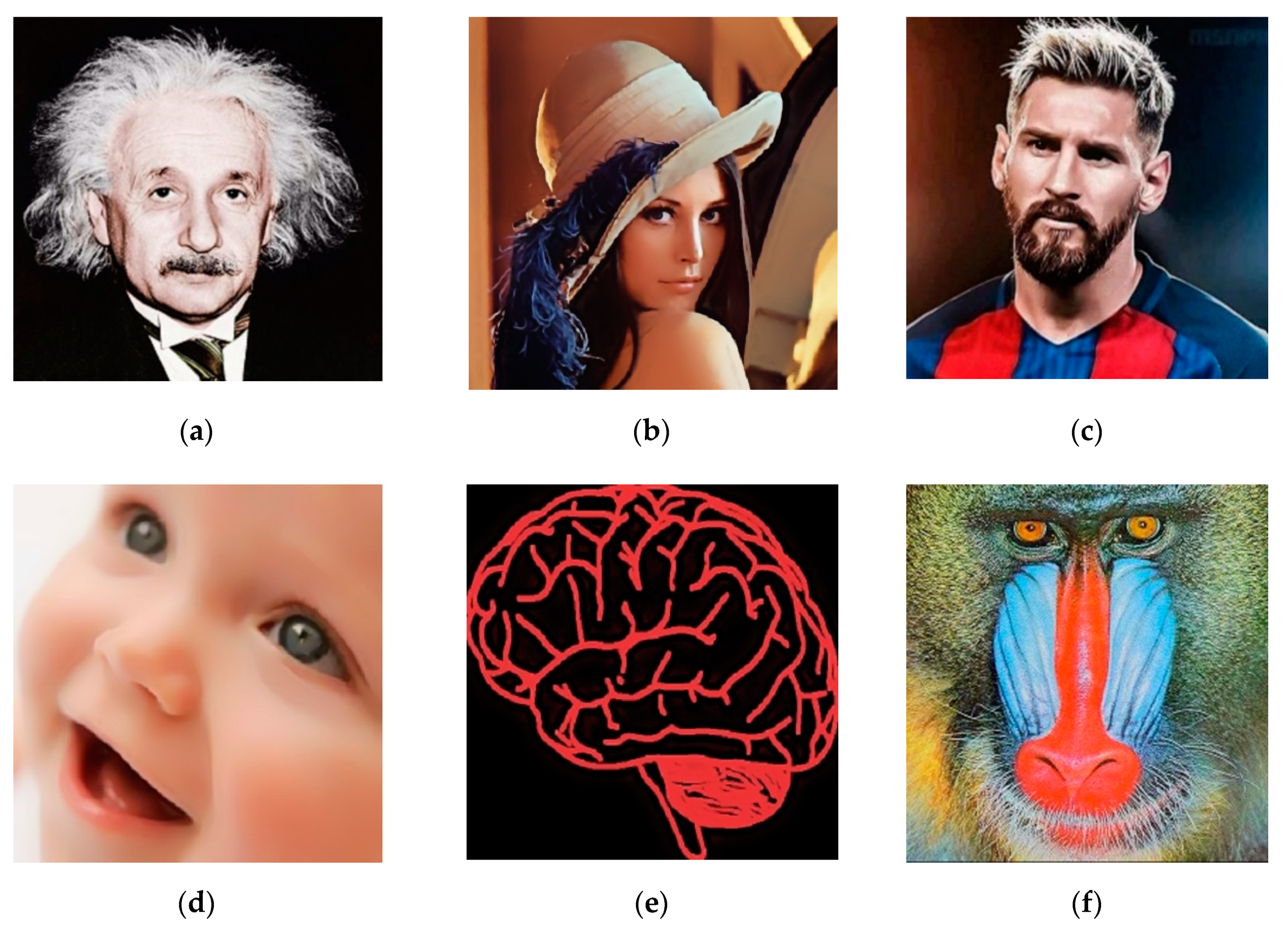
After applying the algorithm on the individual plane, it is then combined into one single RGB image.

4. Results

The above algorithm is applied on different test images and compared with the bi-cubic interpolation technique. Test images were of 512 × 512 dimensions. The performance metrics are PSNR and MSE and qualitative judgment has been done. PSNR is taken as an evaluation measure, it is expressed in dB, and it measures the closeness of the reconstructed image to the original image. Higher the PSNR means the reconstructed image is close enough to the original image. On the other side MSE computes the difference between the reconstructed and original image. Zero MSE suggests that both the images are perfectly matched.

Table 1. PSNR comparison of the bi-cubic and proposed algorithm.

S. No	Test Images	PSNR
		Bi-cubic Interpolation	Proposed Method
1	Lena	32.32	32.83
2	Mona Lisa	23.99	26.37
3	Baboon	24.12	28.37
4	Einstein	30.16	31.05
5	Messi	35.37	37.07
6	Brain	30.58	30.54
7	Baby	37.34	38.76

shows the PSNR of bi-cubic and proposed algorithm, it is clearly observed that proposed algorithm has outperformed the bi-cubic except for the Brain, where bi-cubic shows better performance over proposed method. The MSE comparison is shown in

Table 2. MSE comparison of bi-cubic and proposed algorithm.

S. No	Test Images	PSNR
		Bi-cubic Interpolation	Proposed Method
1	Lena	38.07	37.57
2	Mona Lisa	259	149
3	Baboon	251.2	94.5
4	Einstein	62.5	50.96
5	Messi	18.8	12.74
6	Brain	63.7	62.8
7	Baby	11.9	8.63

, where it is self-explanatory that the proposed algorithm shows better performance over the Bi-cubic, however, the MSE value of bi-cubic for Brain gives better result. Figure 4 and Figure 5 shows the quantitative comparison based on PSNR and MSE. However, qualitative results are shown in Figure 6, Figure 7 and Figure 8. The coding of the proposed method is written and simulated in MATLAB.

The comparison of Bicubic interpolation with the proposed method is measured with PSNR and is represented by Figure 4.

The MSE comparison of the proposed algorithm with the existing bicubic interpolation is shown in Table 2.

Figure 5 represents the comparative results of bicubic interpolation and proposed technique with respect to the mean-squared error values.

The qualitative results have been shown in Figure 5, Figure 6 and Figure 7.

5. Conclusions

A wavelet and spatial domain-based super-resolution algorithm has been developed that recuperates the best high-resolution image equivalent to the input image. Super-resolved images from low-resolution images are acquired by applying bicubic interpolation and the proposed method. The proposed technique gives the best results than the bi-cubic interpolation, since the super-resolved images acquired using bi-cubic interpolation still have the blurring artifacts. We can see the superior performance of the proposed method both visually as well as in terms of PSNR and MSE. On the other hand, the test images of high-resolution give the same results for both the bi-cubic interpolation and the proposed technique. The reason for this might be that the high-resolution images may contain the high-frequency components.

The proposed technique is faster as it takes advantages of both the spatial and wavelet domains. However, other possibilities can be exploited to find efficient methods for up sampling which will, in turn, make some improvements. Texture-based and wavelet domain-based algorithms can be used for up-sampling and some research should be carried out to observe which algorithm performs better for a class of images. In future work, high-resolution images will be targeted with smooth edges to improve the visual quality of the SR images. The technique can also be extended to the super-resolution of videos. This work can be extended by applying different filtering techniques (see [46] and references therein).

References

1. Park, S.C.; Park, M.K.; Kang, M.G. Super-resolution image reconstruction: A technical review. IEEE Signal Process. Mag. 2003, 20, 21–36. [Google Scholar] [CrossRef]
2. Zhu, X.; Wang, X.; Wang, J.; Jin, P.; Liu, L.; Mei, D. Image Super-Resolution Based on Sparse Representation via Direction and Edge Dictionaries. Math. Probl. Eng. 2017, 2017, 3259357. [Google Scholar] [CrossRef]
3. Yue, L.; Shen, H.; Li, J.; Yuan, Q.; Zhang, H.; Zhang, L. Image super-resolution: The techniques, applications, and future. Signal Process. 2016, 128, 389–408. [Google Scholar] [CrossRef]
4. Nasrollahi, K.; Moeslund, T.B. Super-resolution: A comprehensive survey. Mach. Vis. Appl. 2004, 25, 1423–1468. [Google Scholar] [CrossRef]
5. Tian, J.; Ma, K.K. A survey on super-resolution imaging. Signal Image Video Process. 2011, 5, 329–342. [Google Scholar] [CrossRef]
6. Takeda, H.; Milanfar, P.; Protter, M.; Elad, M. Super-resolution without explicit subpixel motion estimation. IEEE Trans. Image Process. 2009, 18, 1958–1975. [Google Scholar] [CrossRef]
7. Ng, M.K.; Shen, H.; Lam, E.Y.; Zhang, L. A total variation regularization based super-resolution reconstruction algorithm for digital video. EURASIP J. Adv. Signal Process. 2007, 1, 074585. [Google Scholar] [CrossRef]
8. Yuan, Q.; Zhang, L.; Shen, H.; Li, P. Adaptive multiple-frame image super-resolution based on U-curve. IEEE Trans. Image Process. 2010, 19, 3157–3170. [Google Scholar] [CrossRef]
9. Liu, C.; Sun, D. On Bayesian adaptive video super resolution. IEEE Trans. Pattern Anal. Mach. Intell. 2014, 36, 346–360. [Google Scholar] [CrossRef]
10. Takeda, H.; Farsiu, S.; Milanfar, P. Kernel Regression for Image Processing and Reconstruction. Ph.D. Thesis, University of California, Santa Cruz, CA, USA, 2006. [Google Scholar]
11. Zhang, H.; Zhang, L.; Shen, H. A blind super-resolution reconstruction method considering image registration errors. Int. J. Fuzzy Syst. 2015, 17, 353–364. [Google Scholar] [CrossRef]
12. Babacan, S.D.; Molina, R.; Katsaggelos, A.K. Variational Bayesian super resolution. IEEE Trans. Image Process. 2011, 20, 984–999. [Google Scholar] [CrossRef]
13. Su, H.; Tang, L.; Wu, Y.; Tretter, D.; Zhou, J. Spatially adaptive block-based super-resolution. IEEE Trans. Image Process. 2012, 21, 1031–1045. [Google Scholar] [PubMed]
14. Mallat, S.G. A theory for multiresolution signal decomposition: The wavelet representation. IEEE Trans. Pattern Anal. Mach. Intell. 1989, 7, 674–693. [Google Scholar] [CrossRef]
15. Rioul, O.; Duhamel, P. Fast algorithms for discrete and continuous wavelet transforms. IEEE Trans. Inf. Theory 1992, 38, 569–586. [Google Scholar] [CrossRef] [Green Version]
16. Newland, D.E. Harmonic wavelet analysis. Proc. R. Soc. Lond. Ser. A Math. Phys. Sci. 1993, 443, 203–225. [Google Scholar] [CrossRef]
17. Dupnchel, L.; Milanfar, P.; Ruckebusch, C.; Huvenne, J.P. Super-resolution and Raman chemical imaging: From multiple low resolution images to a high resolution image. Anal. Chim. Acta 2008, 607, 168–175. [Google Scholar] [CrossRef] [PubMed]
18. Ksomastsu, T.; Aizawa, K.; Igarashi, T.; Saito, T. Signal processing based method for acquiring very high resolution images with multiple cameras and its theoretical analysis. IEEE Proc. I Commun. Speech Vis. 1993, 140, 19–24. [Google Scholar]
19. Li, J.M.; Qu, Y.Y.; Gu, Y.; Fang, T.Z.; Li, C.H. Super-resolution based on fast linear Kernal regression. In Proceedings of the International conference on Machine Learning and Cybernetics, Tianjin, China, 14–17 July 2013; pp. 333–339. [Google Scholar]
20. Parandeh Gheibi, A.; Rahimian, M.A.; Akhaee, M.A.; Ayremlou, A.; Marvasti, F. Compensating for distortions in interpolation of two-dimensional signals using improved iterative techniques. In Proceedings of the 17th International Conference on Telecommunications, Doha, Qatar, 4–7 April 2010; pp. 929–934. [Google Scholar]
21. Temizel, A.; Vlachos, T. Image resolution upscaling in the wavelet domain using directional cycle spinning. J. Electron. Imaging 2005, 14, 040501. [Google Scholar] [Green Version]
22. Woo, D.H.; Eom, I.K.; Kim, Y.S. Image interpolation based on inter-scale dependency in wavelet domain. In Proceedings of the International Conference on Image Processing, Singapore, 24–27 October 2004; pp. 1687–1690. [Google Scholar]
23. Sun, L.; Han, F.; Cai, C.; Su, L. Partially supervised anchored neighborhood regression for image super-resolution through FoE features. Neurocomputing 2018, 275, 2341–2354. [Google Scholar] [CrossRef]
24. Khan, S.; Bianchi, T. Ant Colony Optimiazation (ACO) based Data Hiding in Image Complex Region. Int. J. Electr. Comput. Eng. 2018, 8, 379–389. [Google Scholar]
25. Qiang, Y. Image denoising based on Haar wavelet transform. In Proceedings of the International Conference on Electronics and Optoelectronics, Dalian, China, 29–31 July 2011; Volume 3, pp. V3–V129. [Google Scholar]
26. Deshpande, A.; Patavardhan, P.P.; Rao, D.H. Iterated Back Projection Based Super-Resolution for Iris Feature Extraction. Procedia Comput. Sci. 2015, 48, 269–275. [Google Scholar] [CrossRef] [Green Version]
27. Gormus, E.T.; Canagarajah, C.N.; Achim, A.M. Exploiting spatial domain and wavelet domain cumulants for fusion of SAR and optical images. In Proceedings of the International Conference on Image Processing, Hong Kong, China, 26–29 September 2010; pp. 1209–1212. [Google Scholar]
28. Lee, D.D.; Seung, H.S. Learning the parts of objects by non-negative matrix factorization. Nature 1999, 401, 788–791. [Google Scholar] [CrossRef]
29. Hoyer, P.O.; Hyvärinen, A. A multi-layer sparse coding network learns contour coding from natural images. Vis. Res. 2002, 42, 1593–1605. [Google Scholar] [CrossRef] [Green Version]
30. Hoyer, P.O. Non-negative sparse coding. In Proceedings of the IEEE Workshop on Neural Networks for Signal Processing, Martigny, Switzerland, 4–6 September 2002; pp. 557–565. [Google Scholar]
31. Hoyer, P.O. Non-negative matrix factorization with sparseness constraints. J. Mach. Learn. Res. 2004, 5, 1457–1469. [Google Scholar]
32. Kale, V.U.; Khalsa, N.N. Performance evaluation of various wavelets for image compression of natural and artificial images. Int. J. Comput. Sci. Commun. 2010, 1, 179–184. [Google Scholar]
33. Naik, S.; Borisagar, V. A novel super resolution algorithm using interpolation and lwt based denoising method. Int. J. Image Process. 2012, 6, 198–206. [Google Scholar]
34. Yang, J.; Wright, J.; Huang, T.S.; Ma, Y. Image super-resolution as sparse representation of raw image patches. In Proceedings of the IEEE Conference on Computer Vision and Pattern Recognition (CVPR), Anchorage, AK, USA, 23–28 June 2008. [Google Scholar]
35. Glasner, D.; Bagon, S.; Irani, M. Super-resolution from a single image. In Proceedings of the International Conference on Computer Vision (ICCV), Kyoto, Japan, 27 September–4 October 2009; pp. 349–356. [Google Scholar]
36. Nguyen, N.; Milanfar, P.; Golub, G.H. A computationally efficient super resolution image reconstruction algorithm. IEEE Trans. Image Process. 2001, 10, 573–583. [Google Scholar] [CrossRef] [PubMed]
37. Yang, C.Y.; Huang, J.B.; Yang, M.H. Exploiting self-similarities for single frame super-resolution. In Computer Vision–ACCV 2010, Proceedings of the Asian Conference on Computer Vision (ACCV), Queenstown, New Zealand, 8–12 November 2010; Springer: Berlin/Heidelberg, Germany, 2010; pp. 497–510. [Google Scholar]
38. Yang, M.C.; Wang, Y.C.F. A self-learning approach for single image super-resolution. IEEE Trans. Multimed. 2013, 15, 498–508. [Google Scholar] [CrossRef]
39. Dong, W.; Zhang, L.; Shi, G. Centralized sparse representation for image restoration. In Proceedings of the International Conference on Computer Vision (ICCV), Barcelona, Spain, 6–13 November 2011; pp. 1259–1266. [Google Scholar]
40. Naik, S.; Patel, N. Single image super resolution in spatial and wavelet domain. Int. J. Multimedia Its Appl. 2013, 5, 23–32. [Google Scholar] [CrossRef]
41. Nancy, J.; Wilson, J.; Kumar, K.V. Panoramic dental X-ray image compression using wavelet filters. Int. J. Comput. Sci. Issues 2013, 10, 191–200. [Google Scholar]
42. Arora, R.; Sharma, M.L.; Birla, N.; Bala, A. An Algorithm for image compression using 2D wavelet transform. Int. J. Eng. Sci. Technol. 2011, 3, 2758–2764. [Google Scholar]
43. Kavitha, P. Compression-innovated using wavelets in image. Int. J. Innov. Res. Comput. Commun. Eng. 2013, 1, 221–230. [Google Scholar]
44. Irani, M.; Peleg, S. Improving resolution by image registration. CVGIP Graph. Models Image Process. 1991, 53, 231–239. [Google Scholar] [CrossRef]
45. Makwana, R.R.; Mehta, N.D. Single image super-resolution via iterative back projection based Canny edge detection and a Gabor filter prior. Int. J. Soft Comput. Eng. 2013, 3, 379–384. [Google Scholar]
46. Shang, Y. Resilient multiscale coordination control against adversarial nodes. Energies 2018, 11, 1844. [Google Scholar] [CrossRef]
Figure 1. Down-sampling of high-resolution image to obtain the down-sampled image.
Symmetry 11 00464 g001
Figure 2. Up-sampling process of images.
Symmetry 11 00464 g002
Figure 3. Simple iterative back projection method.
Symmetry 11 00464 g003
Figure 4. PSNR comparison of bicubic interpolation and the proposed method.
Symmetry 11 00464 g004
Figure 5. MSE comparison of bicubic interpolation and the proposed method.
Symmetry 11 00464 g005
Figure 6. Original true color image: (a) Einstein; (b) Lena; (c) Messi; (d) baby; (e) brain; (f) baboon.
Symmetry 11 00464 g006
Figure 7. Super-resolved images using the proposed algorithm: (a) Einstein; (b) Lena; (c) Messi; (d) baby; (e) brain; and(f) baboon.
Symmetry 11 00464 g007
Figure 8. Bi-cubic interpolated images: (a) Einstein; (b) Lena; (c) Messi; (d) baby; (e) brain; and (f) baboon.
Symmetry 11 00464 g008