Self-Adaptive Fault Feature Extraction of Rolling Bearings Based on Enhancing Mode Characteristic of Complete Ensemble Empirical Mode Decomposition with Adaptive Noise

Abstract

Originally, a rolling bearing, as a key part in rotating machinery, is a cyclic symmetric structure. When a fault occurs, it disrupts the symmetry and influences the normal operation of the rolling bearing. To accurately identify faults of rolling bearing, a novel method is proposed, which is based enhancing the mode characteristics of complete ensemble empirical mode decomposition with adaptive noise (CEEMDAN). It includes two parts: the first is the enhancing decomposition of CEEMDAN algorithm, and the second is the identified method of intrinsic information mode (IIM) of vibration signal. For the first part, the new mode functions (CIMFs) are obtained by combing the adjacent intrinsic mode functions (IMFs) and performing the corresponding Fast Fourier Transform (FFT) to strengthen difference feature among IMFs. Then, probability density function (PDF) is used to estimate FFT of each CIMF to obtain overall information of frequency component. Finally, the final intrinsic mode functions (FIMFs) are obtained by proposing identified method of adjacent PDF based on geometrical similarity (modified Hausdorff distance (MHD)). FIMFs indicate the minimum amount of mode information with physical meanings and avoid interference of spurious mode in original CEEMDAN decomposing. Subsequently, comprehensive evaluate index (Kurtosis and de-trended fluctuation analysis (DFA)) is proposed to identify IIM in FIMFs. Experiment results indicate that the proposed method demonstrates superior performance and can accurately extract characteristic frequencies of rolling bearing.

1. Introduction

Rolling bearings are a key part of rotary machines and are directly related to machine health status. Thus, it is very essential to introduce an effective method to accurately detect potential abnormalities in bearing. Failure to take such measures risks the occurrence of unexpected and potentially disastrous events [1,2,3].

Currently, vibration analysis technology plays important effect on fault diagnosis domain of rolling bearing. However, traditional signal analysis method (such as Fast Fourier Transform (FFT)) is not suitable for processing vibration signals because of its non-stationary and non-linear characteristics [4]. Wavelet transform is another typical application in the fault diagnosis domain [5,6]. However, it is difficult to select a wavelet base function. Afterwards, empirical mode decomposition (EMD) was introduced by Huang to process the signal which has complex non-linear and non-stationary characteristic [7]. This method can automatically decompose a complicated signal into sets of intrinsic mode function (IMFs). Each IMF is a mono-component and represents a characteristic of modulated amplitude signal. However, EMD presents drawbacks in terms of end effects and mode mixing. For phase-amplitude coupling (PAC) assessment [8], the drawbacks can lead to in--nacuracy in frequency resolution; for signals with shape edges and spikes, it can lead to potential spurious amplitude–amplitude coupling (AAC) [9]. Thus, when it is used to analyze fault signals, it is also limited in terms of extracting characteristic information for rolling bearings. To overcome these drawbacks, Deering et al. [10] and Yeh et al. [11] used a masking signal to improve the decomposed performance of EMD. Reference [11] indicates that the essential relation was illustrated quantifiably between low- and high- frequency bands using the masking phase and amplitude coupling method. However, the authors did not adequately check the choosing procedure of a proper masking signal. Afterwards, Wu et al. [12] and Yeh et al. [13] proposed the ensemble EMD (EEMD) and Complementary EEMD (CEEMD) methods, respectively. However, EEMD and CEEMD bring new issues of spurious modes, because of interactions of added noise and signal in signal decomposition. Then, Torres [14] introduced a complete EEMD with an adaptive noise (CEEMDAN) method to alleviate the drawbacks of EEMD and CEEMD. However, when CEEMDAN is used to analyze the vibration signal, two issues were observed: (1) how to obtain mode information of the original signal with physical meanings; (2) how to identify the IIM of the vibration signal.

(1) On the issue of decomposing an intrinsic mode function with physical meaning

When the vibration signal is decomposed by CEEMDAN, it is necessary to determine two critical parameters: the first is the amplitude of added white noise, and the other is ensemble trails. Lei et al. [15,16] and Zhou et al. [17] believe that no specific expression is used to guide the choice of the two parameters. Chang et al. [18], Zhang et al. [19] and Zvokelj et al. [20] use the signal-noise ratio (SNR) to choose a corresponding amplitude. However, it is assumed that the signal can be analyzed. For vibration signals, Zvokelj et al. [21] still apply experimental methods to judge the amplitude; this may result in added noise not being fully eliminated, and in the decomposed IMFs containing the interference component because of interactions between the added noise and the signal. Finally, although CEEMDAN can avoid mode mixing, it also produces over-decomposition. When IMFs are used to extract fault features, they contain interference frequency components that influence the extraction of the actual bearing fault. To avoid the drawbacks associated with the use of spurious mode, Marcelo et al. [22] proposed a method to extract the k-th IMF by adding an EMD decomposed mode. Although this method may reduce residual noise and obtain more modes with physical meanings, it still has interference in the spurious mode. Yang et al. [23] introduced ensemble local mean decomposition (ELMD) to address the drawbacks of mode mixing in local mean decomposition (LMD). However, the ELMD still has the problem of residue noise and spurious mode. Afterwards, Wang et al. [24] developed a complete ensemble local mean decomposition with adaptive noise (CELMDAN) to avoid the drawbacks in ELMD. However, the CELMDAN still suffers from the same problems as CEEMDAN. Thus, the LMD improved versions (ELMD and CELMDAN) are not also suitable for decomposing vibration signals. Gao et al. [25] proposed combining the methods of adjacent IMFs to obtain a minimum number IMFs with physical meanings; however, this method only relies on IMFs obtaining combined IMF, and the results may introduce distorted information, thereby impeding accurate fault feature extraction.

(2) Issue of identifying IIM among IMFs

Generally, the main fault information of bearing rolling concentrates on one CIMF. A proper method must be developped to find this mode. Traditionally, Kurtosis [26] is sensitive to vibration signals. However, when a fault become severe, it is not consistent with the development of a fault. The correlation coefficient [27,28] and Kullback-Leibler (K-L) divergence [29,30,31] do not work well for identifying faults. Recently, sample entropy (SE) [32,33], approximate entropy (AE) [34,35] and fuzzy entropy (FE) [36,37] were introduced into the fault diagnosis domain. However, at the boundary, SE is changed suddenly and not continuously. AE has the drawback of being heavily reliant upon the data length. FE originates in membership functions, and the function is difficult to determine.

Generally, there were two fault diagnosis methods: one is the discriminant method based on the model, and the other is based on the feature frequency. The former combines artificial intelligence and statistical approaches, such as artificial neural networks (ANN), principal component analysis (PCA), fuzzy logic, Kalman filters and so on, to set up a discriminant model to extract fault [38,39]. For example, Nguyen et al. [40] proposed percentile measurements and a gamma process model to estimate the remaining useful life (RUL) in batch manufacturing processes. Samir et al. [41] proposed a dynamic model to generate fault indicators to identify a cluster for each operation state. This method estimates RUL without prior knowledge. For the second method, Wang et al. [24] first employed ELMD and CELMDAN to decompose the vibration signal and to obtain mode components of the vibration signal, respectively. Then, the kurtosis maximum principle was used to identify IIM and for analyses of the envelope spectrum for IIM. The method can extract fault features, but there are some interference spectra. Li et al. [42] introduced a method based on frequency band entropy to solve the selected problem of IIM. However, the final results showed that the different identified method leads to big differences in the extracted fault frequency.

To overcome the above problem, firstly, this paper proposes a method automatically combining IMFs into a minimum number of IMFs with physical meanings to enhance CEEMDAN decomposition. Here, this method produces new mode function (CIMFs) by combining adjacent IMFs; then, the FFT is done for each CIMF to enhance the difference features of the frequency component in IMFs; all information can then be reflected by PDF estimation. The difference of CIMFs is qualified by MHD [43] to obtain new IMFs with a minimum number and physical meanings. Finally, the comprehensive evaluated index based on Kurtosis and de-trended fluctuation analysis (DFA) [44,45,46] was proposed for the extraction of vibration IIMs. The experiment results show that the proposed method outperforms the other methods for rolling bearing fault diagnoses.

The remainder of this paper is organized as follows: Section 2 introduces the related works to illustrate the principles of existing algorithms; Section 3 describes proposed works (enhancing decomposed algorithm of CEEMDAN and identifying IIM algorithm); Section 4 evaluates the performance of the proposed method for fault diagnosis; Section 5 is the conclusion.

2. Related Works

2.1. CEEMDAN Algorithm

It is well known that EMD [7] has the drawback of mode mixing and end effect. EEMD [12] was introduced to solve this problem. However, it introduces residual noise into the IMFs and produces a spurious mode. To alleviate these phenomena, CEEMDAN [14] was introduced to decompose non-liner and non-stationary signals. Currently, this method is also widely applied in the fault diagnosis domain to obtain feature information on vibration signals [47,48]. The following is the basic principle of CEEMDAN:

(1)

Apply EMD to decompose signal ($x\left(t\right)+w_0{\epsilon }^i\left(t\right)$) to extract the first IMF;

$$c_1\left(t\right)=\frac{1}{N}{\displaystyle \sum _{i=1}^N{c}_1^i\left(t\right)}\hspace{1em}i\in \left\{1,\dots ,N\right\}$$

(1)

Here, $\epsilon \left(t\right)$ is white noise with unit variance, and $w_0$ is the corresponding amplitude.

(2)

Obtain the differential signal by Equation (2);

$$r_1\left(t\right)=x\left(t\right)-c_1\left(t\right)$$

(2)

(3)

Extract the first mode by decompose $r_1\left(t\right)+w_1{E}_1\left({\epsilon }^i\left(t\right)\right)$ and appoint the second IMF using Equation (3);

$$c_2\left(t\right)=\frac{1}{N}{\displaystyle \sum _{i=1}^N{E}_1}\left(r_1\left(t\right)+w_1{E}_1\left({\epsilon }^i\left(t\right)\right)\right)$$

(3)

(4)

Decompose the $k$-th residue and extract the first mode, and the $\left(k+1\right)$-th mode can be obtained using the following equation ($k=2,\dots ,K$):

$$c_{k+1}\left(t\right)=\frac{1}{N}{\displaystyle \sum _{i=1}^N{E}_1}\left(r_k\left(t\right)+w_k{E}_k\left({\epsilon }^i\left(t\right)\right)\right)$$

(4)

Here, $E_k(\cdot )$ indicates the symbol function of the k-th IMF.

(5)

Obtain last mode by Equation (5) when the residue has fewer than (or equal to) two extrema by repeating step,

$$R\left(t\right)=x\left(t\right)-{\displaystyle \sum _{k=1}^K{c}_k\left(t\right)}$$

(5)

Signal $x\left(t\right)$ is decomposed using equation,

$$x\left(t\right)={\displaystyle \sum _{k=1}^K{c}_k\left(t\right)}+R\left(t\right)$$

(6)

2.2. De-Trended Fluctuation Algorithm (DFA)

Recently, DFA [44] has been known as a sales tool, and has been used to analyze non-stationary signals, especially for the volatility of time series. The DFA principle is as follows:

(1)

Divide the following series into integrated time:

$$y\left(k\right)={\displaystyle \sum _{i=1}^k\left[x\left(i\right)-\overline{x}\right]}\hspace{1em}k=1,2,3,\dots ,N$$

(7)

Here, $\overline{x}$ indicates the mean of the series $x\left(i\right)$.

(2)

Slice $y\left(k\right)$ into n length sub-section;

(3)

Apply least square method fitting to obtain the local trend $y_n\left(k\right)$;

(4)

Extract $y_n\left(k\right)$ from the $y\left(k\right)$ to obtain fluctuation function $F\left(n\right)$;

$$F\left(n\right)={\left(\frac{1}{N}{\displaystyle \sum _{k=1}^N{\left[y\left(k\right)-y_n\left(k\right)\right]}^2}\right)}^{\frac{1}{2}}$$

(8)

(5)

Obtain different $F\left(n\right)$ by different length segments;

(6)

Calculate the slope $\alpha$ (fractal scaling index) between $\log \left(F\left(n\right)\right)$ and $\log \left(k\right)$; the bigger slope $\alpha$ of signal, the smoother time series (as shown in Equation (9)):

$$F\left(n\right)\propto n^{\alpha }$$

(9)

2.3. Modified Hausdorff Distance (MHD)

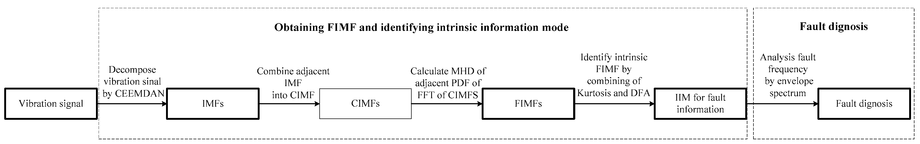
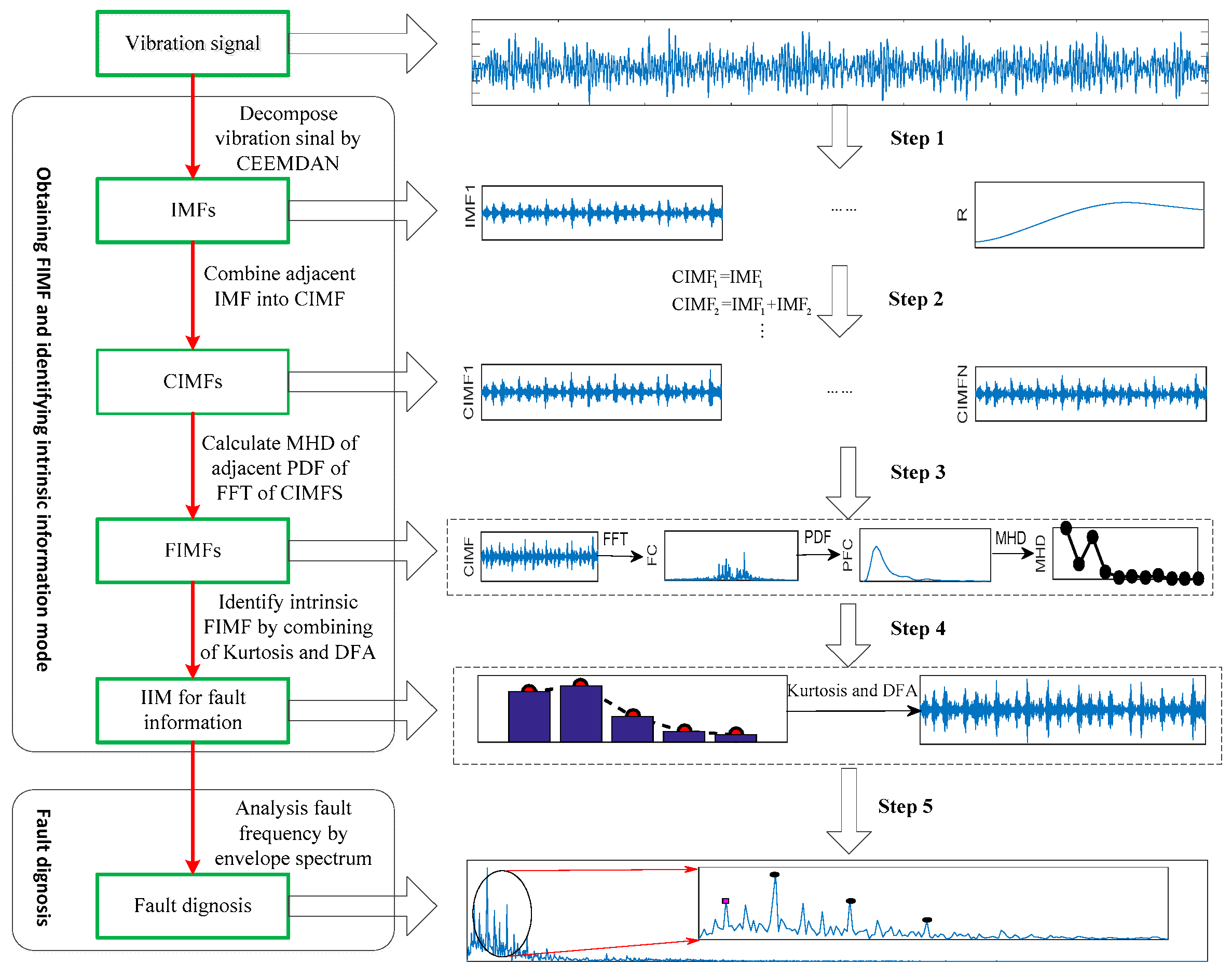
Hausdorff distance (HD) [49] was first used in image processing. HD computes the similarity between two objects [50,51]. The quantity principle is based on object shape. The following expression is the distance of two point ($a$ and $b$):

$$d\left(a,b\right)=\Vert a-b\Vert$$

(10)

Then, the distance between a point $a$ and a set of points $\mathrm{B}=\left\{b_1,\dots ,b_{N_b}\right\}$ is defined as:

$$d\left(a,B\right)=mi{n}_{b\in B}\Vert a-b\Vert$$

(11)

The Equation (11) is defined as direct distance between two series $\mathrm{A}=\left\{a_1,\dots ,a_{N_a}\right\}$ and $\mathrm{B}=\left\{b_1,\dots ,b_{N_b}\right\}$:

$$d_1\left(A,B\right)=\underset{a\in A}{max}d\left(a,B\right)$$

(12)

The modified directed distance (MHD) can been obtained using the following equation:

$$d_2\left(A,B\right)=\frac{1}{N_a}{\displaystyle \sum }_{a\in A}d\left(a,B\right)$$

(13)

The Equation (13) is the undirected distance:

$$\mathrm{f}\left(\mathrm{d}\left(A,B\right),\mathrm{d}\left(B,A\right)\right)=\max \left(\mathrm{d}\left(A,B\right),\mathrm{d}\left(B,A\right)\right)$$

(14)

Thus, the modified Hausdorff distance (MHD) is the $\mathrm{MHD}=\mathrm{f}\left(d_2\left(A,B\right),d_2\left(B,A\right)\right)$. When the signal is influenced by noise, MHD can obtain the real distance.

3. Proposed Works

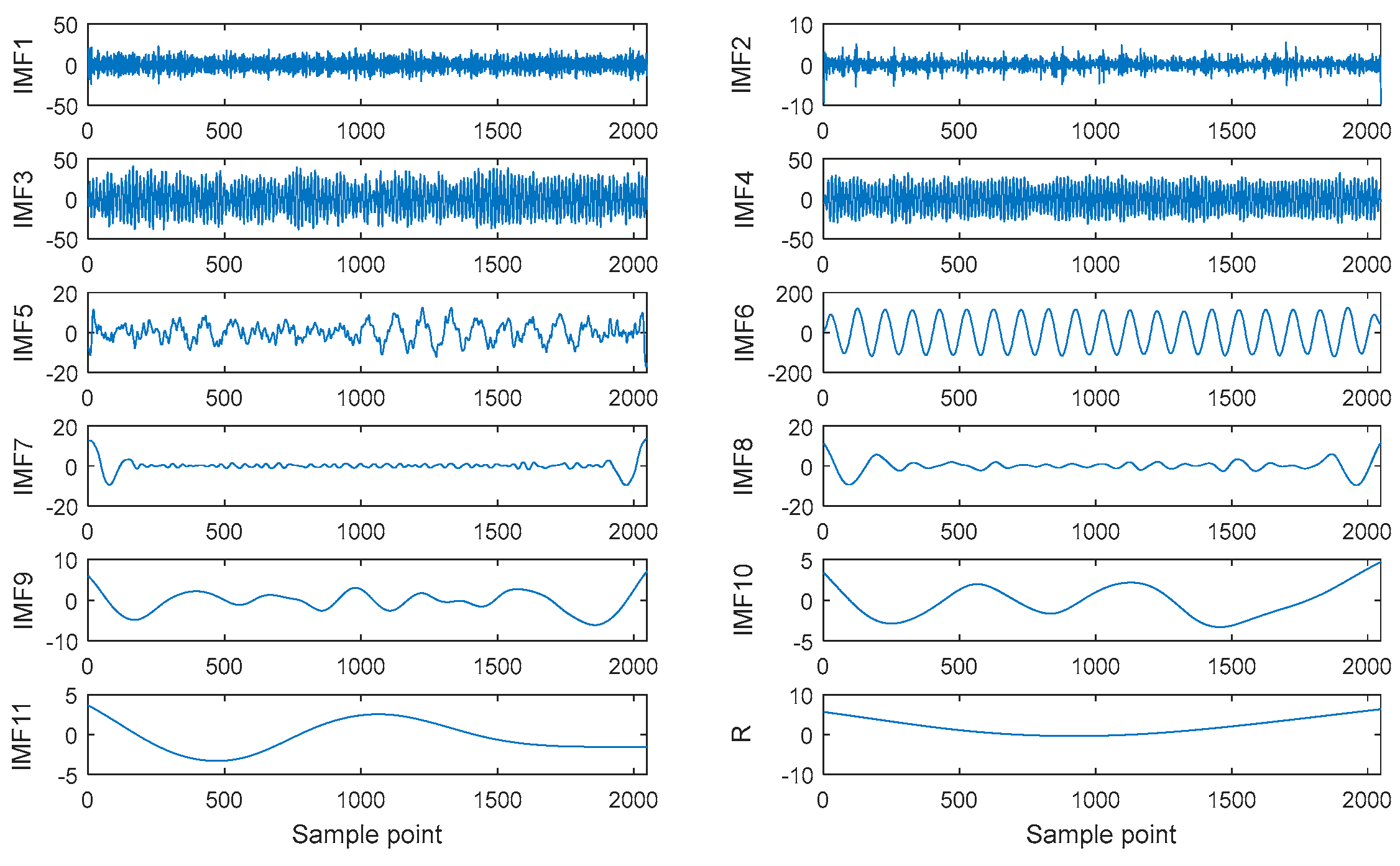
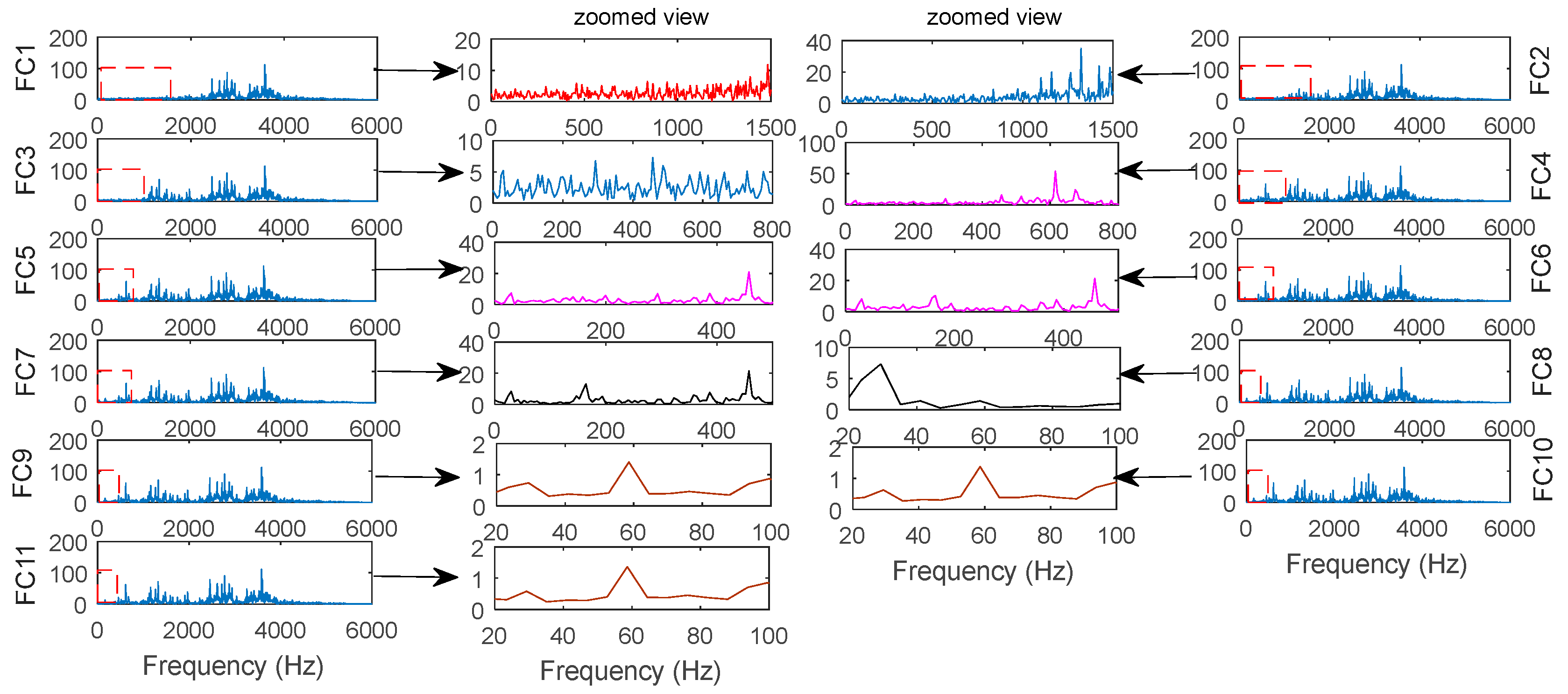
3.1. Identifying of IMF with Minimum Number and Physical Meaning

In this section, a method is proposed to obtain the minimum number of IMFs and physical meanings based on frequency characteristics of IMFs. Firstly, it combines the adjacent IMFs into new modes (sign as CIMFs). Then, a FFT analysis is performed for each CIMF (obtained waveform is sign as FC). In this way, the FFT can organize the IMF containing the same or similar frequency bands into a class. In addition, because a PDF can reflect a state of knowledge of the desired signal rather than only a frequency based on Bayesian theory, a PDF contains complete information about the FC, and is expected to capture the feature information of FCs (sign as PFC). Finally, the similarity is quantized by the MHD of the adjacent PFC to adaptively obtain the final IMFs (FIMFs).

Here, the following simulated signal is introduced to illustrate the identified process.

$$x\left(t\right)=A_{1}sin\left(2\pi f_{1}t\right)+A_{2}sin\left(2\pi f_{2}t\right)+n\left(t\right)$$

(15)

In Equation (15), the amplitude $A_1$ and $A_2$ are 120 and 50, and frequency $f_1$ and $f_2$ are 10 Hz and 75 Hz, respectively. $n\left(t\right)$ obey distribution $N\left(0,{11}^2\right)$. The sample frequency is 1 kHz, and the data length is 20148 (as shown Figure 1).

Theoretically, the four IMFs should be obtained through the decomposition of signal $x\left(t\right)$ (the first is the noise component, the second is the IMF with a frequency component of 75 Hz, the third is that of 10 Hz, and last one is residue). However, it was found that twelve IMFs were obtained by CEEMDAN decomposition (as shown Figure 2). Here, the amplitude of white noise is 0.2, and the ensemble size is 100; this means that there are some spurious modes because of the interactions between the signal and the added noise. It is difficult to identify real frequency information of the original signal after it had been subjected to the interference of spurious mode. To solve this problem, the proposed method is introduced to automatically distinguish the frequency components of the simulated signal. Firstly, the adjacent IMFs are combined by Equation (16) to obtain the CIMFs (as shown Figure 3).

$$\begin{array}{l}{\mathrm{CIMF}}_1{=\mathrm{IMF}}_1\\ {\mathrm{CIMF}}_2{=\mathrm{IMF}}_1{+\mathrm{IMF}}_2\\ {\mathrm{CIMF}}_3{=\mathrm{IMF}}_1{+\mathrm{IMF}}_2{+\mathrm{IMF}}_3\\ \hspace{1em}\hspace{1em}\hspace{1em}\hspace{1em}\hspace{1em}⋮\\ {\mathrm{CIMF}}_{n-1}{=\mathrm{IMF}}_1+{\mathrm{IMF}}_2+{\mathrm{IMF}}_3\dots +{\mathrm{IMF}}_{n-1}\end{array}$$

(16)

Next, FFT is used to extract the frequency component of the CIMF. Here, the waveform, which is obtained by FFT of CIMF, is referred to as FC. To distinguish the feature difference among FCs, the main frequency band (the dotted box in Figure 4), which contains from 0 Hz to 100 Hz in all FCs, is enlarged (except the frequency band from 100 Hz to 500 Hz for FC1 and FC2). Figure 5 illustrates the frequency spectrum and amplitude information of the original and enlarged FC. It was found that the frequency spectrum of FC1 is same as that of FC2, and that the maximum amplitude of FC1 is less than that of FC2. Among FC3, FC4 and FC5, the frequency spectra were similar. However, the maximum amplitude of FC3 is less than that of FC4 and FC5; the residue FCs (FC6, FC7, FC8, FC9, FC10 and FC11) are identical; this means that the IMF1 and IMF2 can been divided into a class, as can IMF6, IMF 7, IMF 8, IMF 9, IMF 10 and IMF 11. However, it is impossible to determine whether IMF3, IMF4 and IMF5 may also organized into a class. Next, the PDF and MHD were used to enhance their feature difference and quantify classification results.

Here, the PDF is used to estimate each FC (the obtained waveform is designated as PFC) to enhance discernment of the difference features among FCs (especially for FC3, FC4 and FC5) and subsequent quantitative ability. Figure 5 shows the estimated PDF and local zoom of the interest components in each PFC. It was found that the geometry feature of each PFC was more obvious than that of the corresponding FC.

Finally, modified Hausdorff distance (MHD) is used to calculate the geometry distance between adjacent PFCs (as shown Figure 6).

The second and fifth indices of MHD are the local maxima; this means that CIMF₂ and CIMF₃, CIMF₅ and CIMF₆ are not similar. CIMF₂ combines IMF₁ and IMF₂, and CIMF₃ combines IMF₁, IMF₂ and IMF₃; this illustrates that IMF₃ is not similar to IMF₁ and IMF₂. Likewise, IMFs after IMF₆ are not similar to IMF₃, IMF₄ and IMF₅; this means that the IMF₃, IMF₄ and IMF₅ can been organized into a class. Figure 7 shows a relational graph of CIMFs (‘Y’ means that there is a similarity among adjacent CIMFs, while ‘N’ means non-similarity). Thus, the CIMFs are obtained using following equation:

$$\begin{array}{l}{\mathrm{CIMF}}_1={\mathrm{IMF}}_1+{\mathrm{IMF}}_2\\ {\mathrm{CIMF}}_2{=\mathrm{IMF}}_3{+\mathrm{IMF}}_4{+\mathrm{IMF}}_5\\ {\mathrm{CIMF}}_3{=\mathrm{IMF}}_6{+\mathrm{IMF}}_7{+\mathrm{IMF}}_8{+\mathrm{IMF}}_9{+\mathrm{IMF}}_{10}{+\mathrm{IMF}}_{11}\\ {\mathrm{CIMF}}_4=\mathrm{R}\end{array}$$

(17)

Figure 8 is the final combined FIMF and corresponding Fast Fourier transform (FFT). It was found that the identified frequency component of FIMF₂ and FIMF₃ are almost in accordance with theoretic frequencies in Equation (15) (75 Hz and 10 Hz). The FIMF₁ and R are the noisy IMF and residue, respectively; this proves that the proposed method can be used to distinguish the frequency components of a complicated signal and avoid the interference of spurious mode.

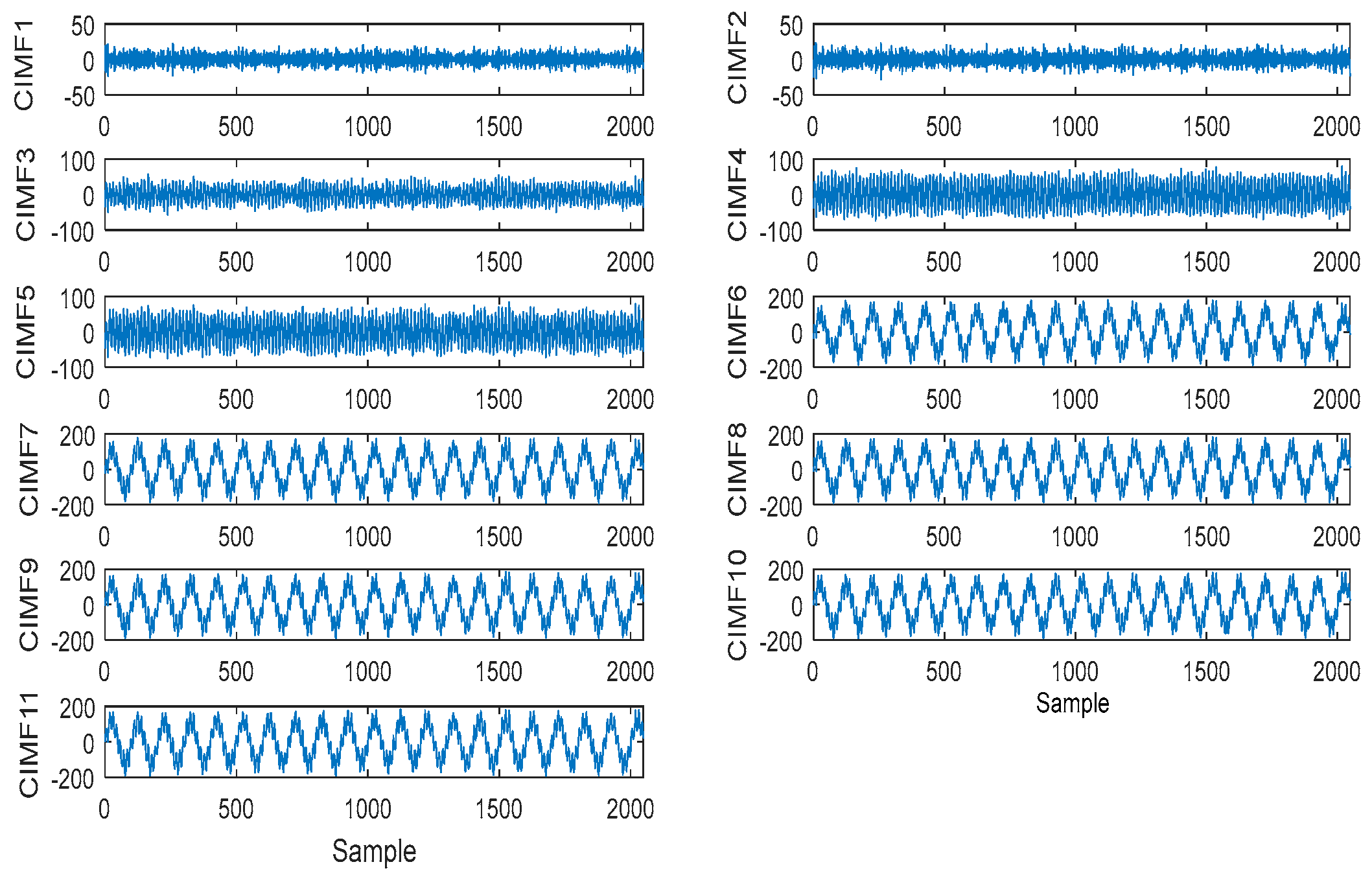
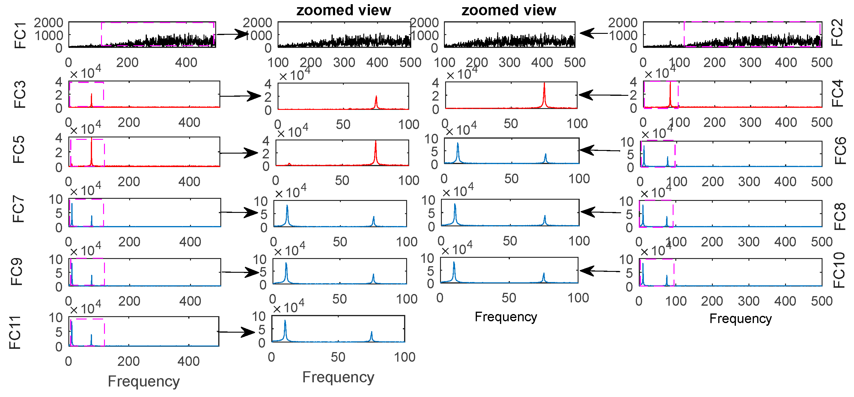
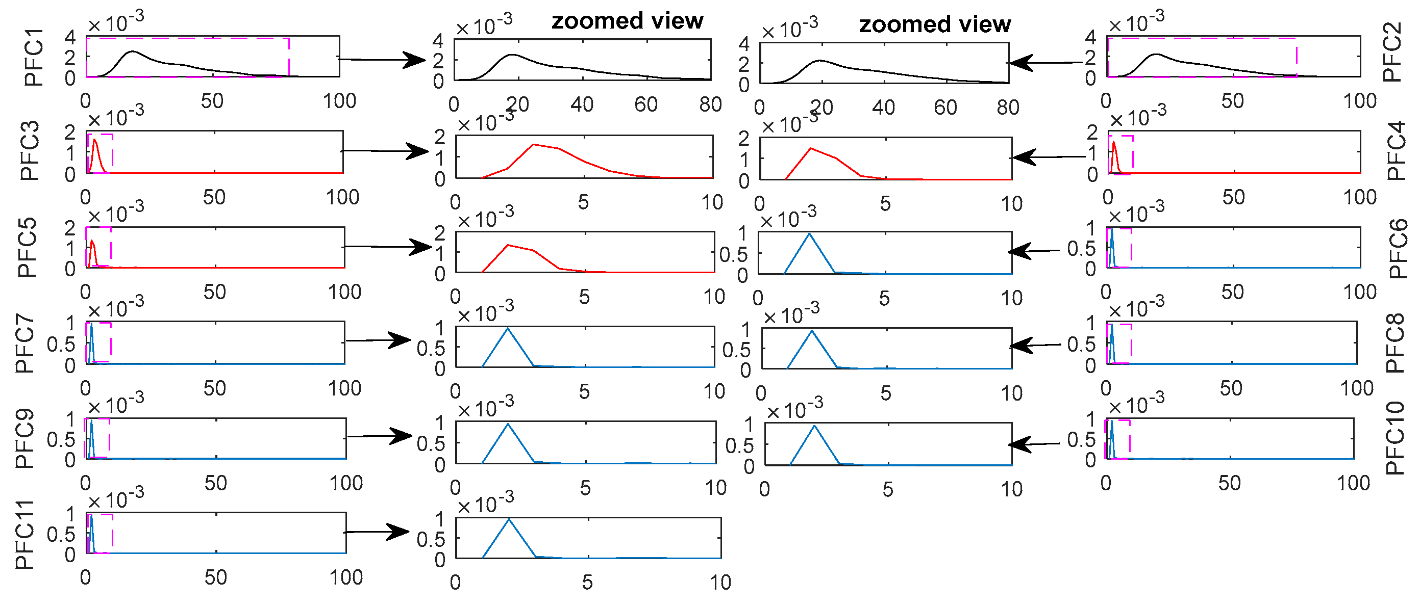
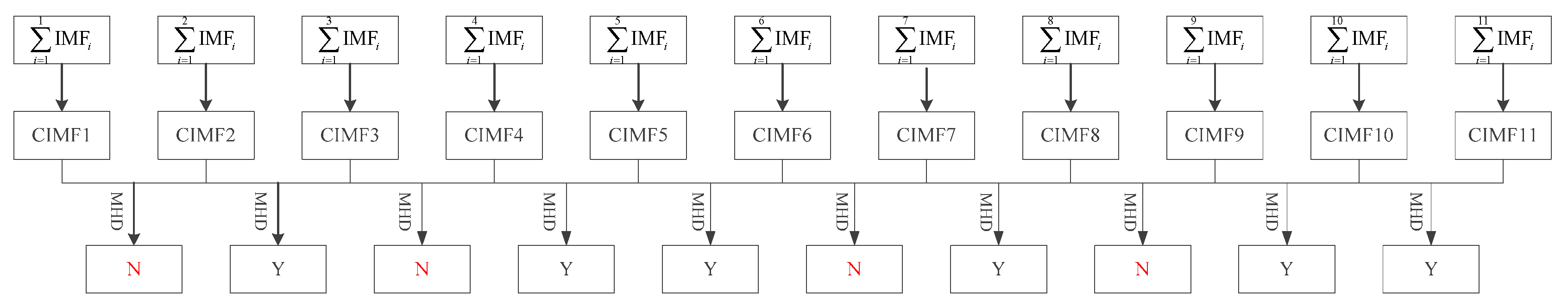
3.2. Selection of Intrinsic Information Mode

Generally, only one FCMF contains the main intrinsic information of bearing faults in FCIMFs. Thus, it was necessary to develop a proper method to identify the FCMF. Traditionally, Kurtosis [26] is often used to indicate the features of an impulse signal and to extract early faults in rolling bearings. However, Kurtosis does not indicate the fault level when it becomes more serious. The expression of Kurtosis is as follows:

$$\mathrm{Kur}=\frac{E{\left(x-\mu \right)}^4}{{\sigma }^4}$$

(18)

Here, $\mu$ indicates the mean, $\sigma$ is the standard deviation and $E(\cdot )$ is expectation operator. Recently, DFA [44] has been used to reflect fluctuation of time series, especially for non-stationary signals such as vibration signals; the more seriousness the bearing fault, the larger fluctuation of the vibration signal, and the larger the DFA (see Section 2.2 for more information). This means that DFA can been used to evaluate the degree of seriousness of the bearing fault. Thus, this paper proposes a comprehensive evaluation index, $S_i$, which combines Kurtosis and DFA, to select IIM in FIMFs.

$$S_i=\frac{k{u}_i\cdot {\alpha }_i}{{\displaystyle \sum _{i=1}^{N_F}k{u}_i}\cdot {\displaystyle \sum _{i=1}^{N_F}{\alpha }_i}}$$

(19)

Here, $k{u}_i$ and ${\alpha }_i$ denote the $i$-th values of Kurtosis and DFA, respectively, $N_F$ indicates the number of FIMFs.

The proposed method is presented as follows, and a flow chart is shown in Figure 9:

(1)

Decompose the vibration signal into sets of IMFs by CEEMDAN;

(2)

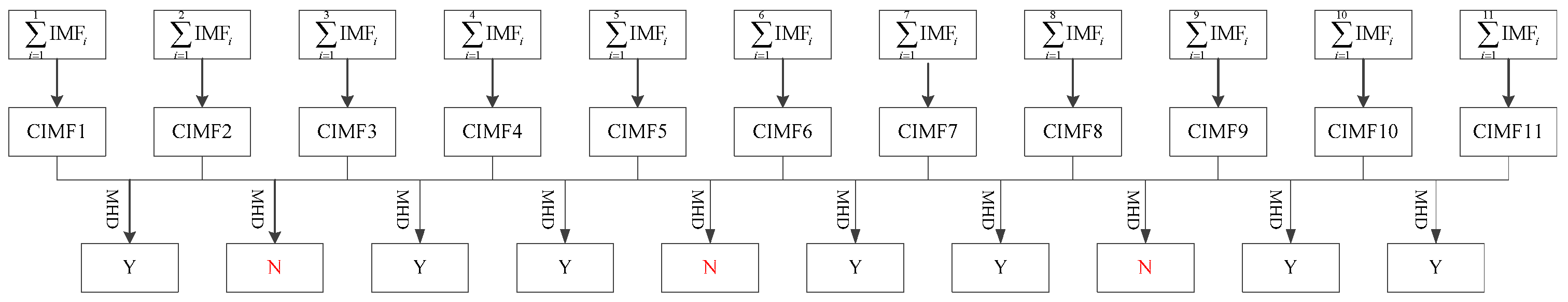
Combine the adjacent IMFs into CIMF;

(3)

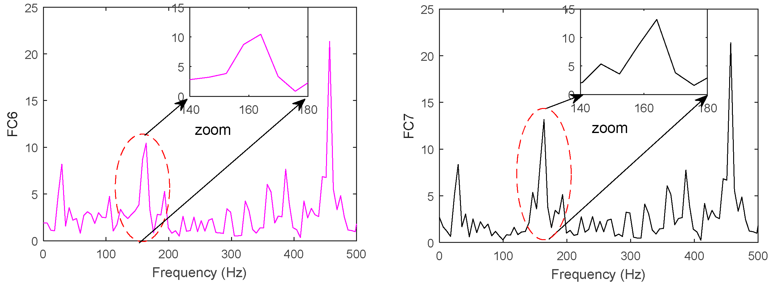
Obtain the FC by calculating the FFT of each CIMF;

(4)

Get PFC by estimating the PDF of each FFT;

(5)

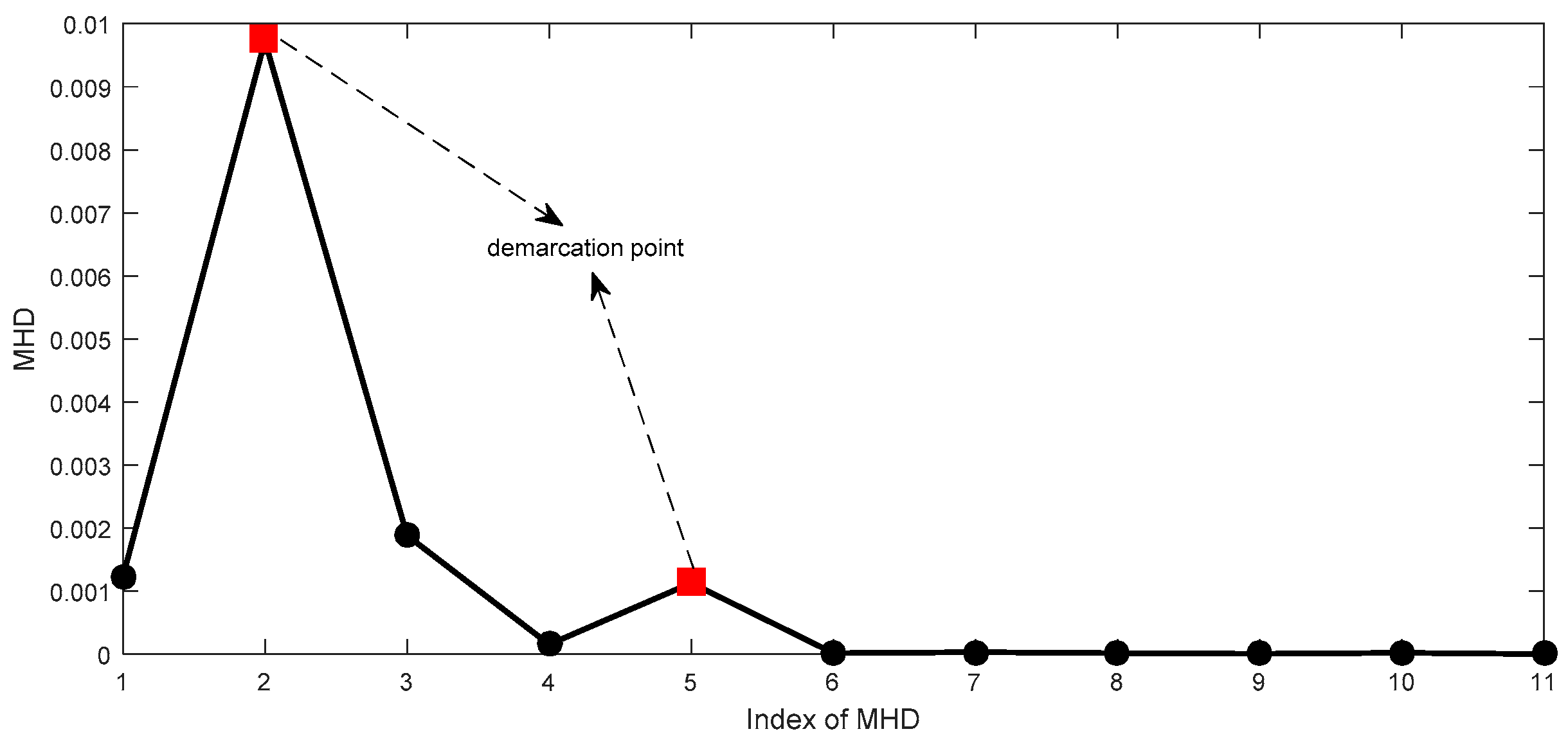
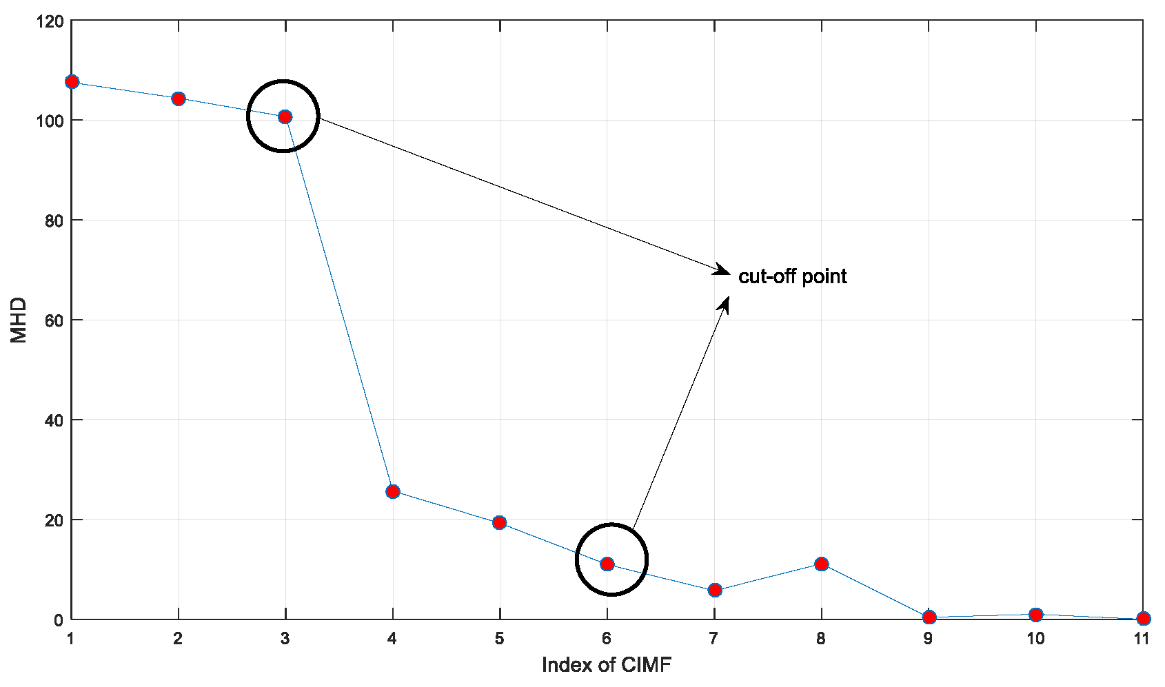
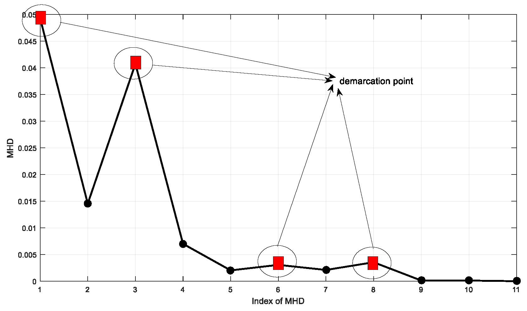
Obtain the FIMF by calculating the MHD of adjacent PDF;

(6)

Obtain the minimum amount of mode information with physical meanings;

(7)

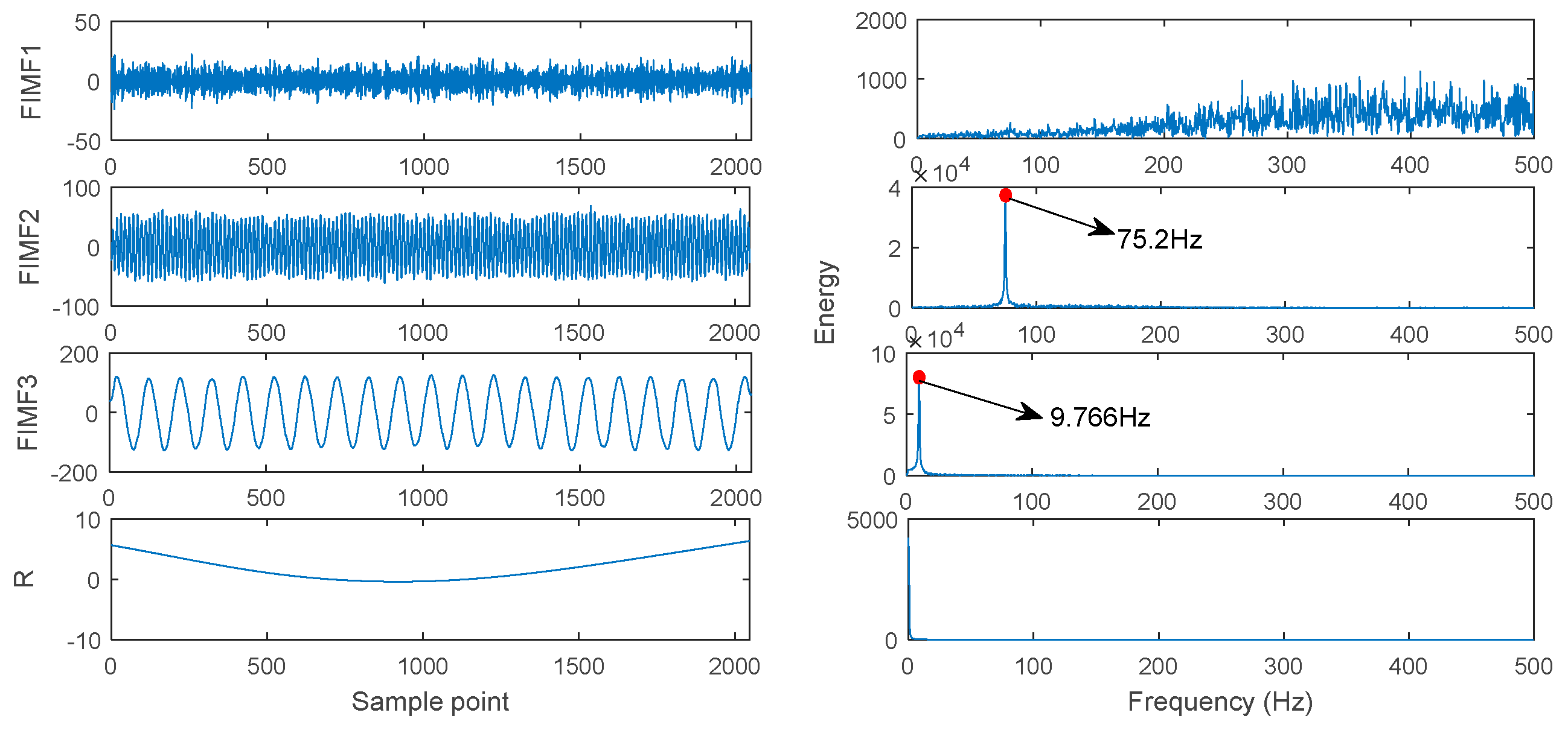
Identify the IIM by comprehensive evaluate index;

(8)

Identify the feature frequency of rolling bearings using the IIM envelope.

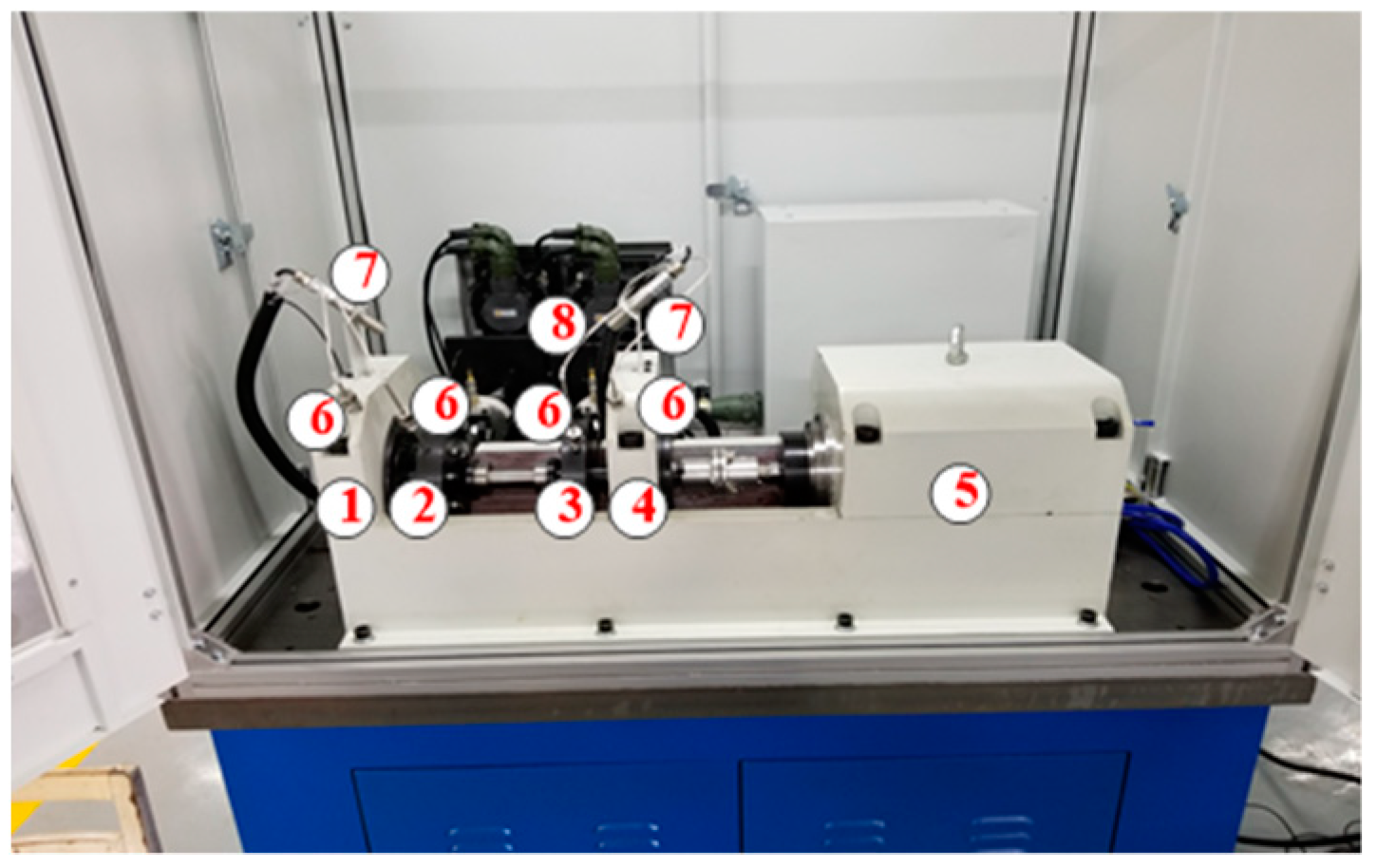
4. Results and Discussions

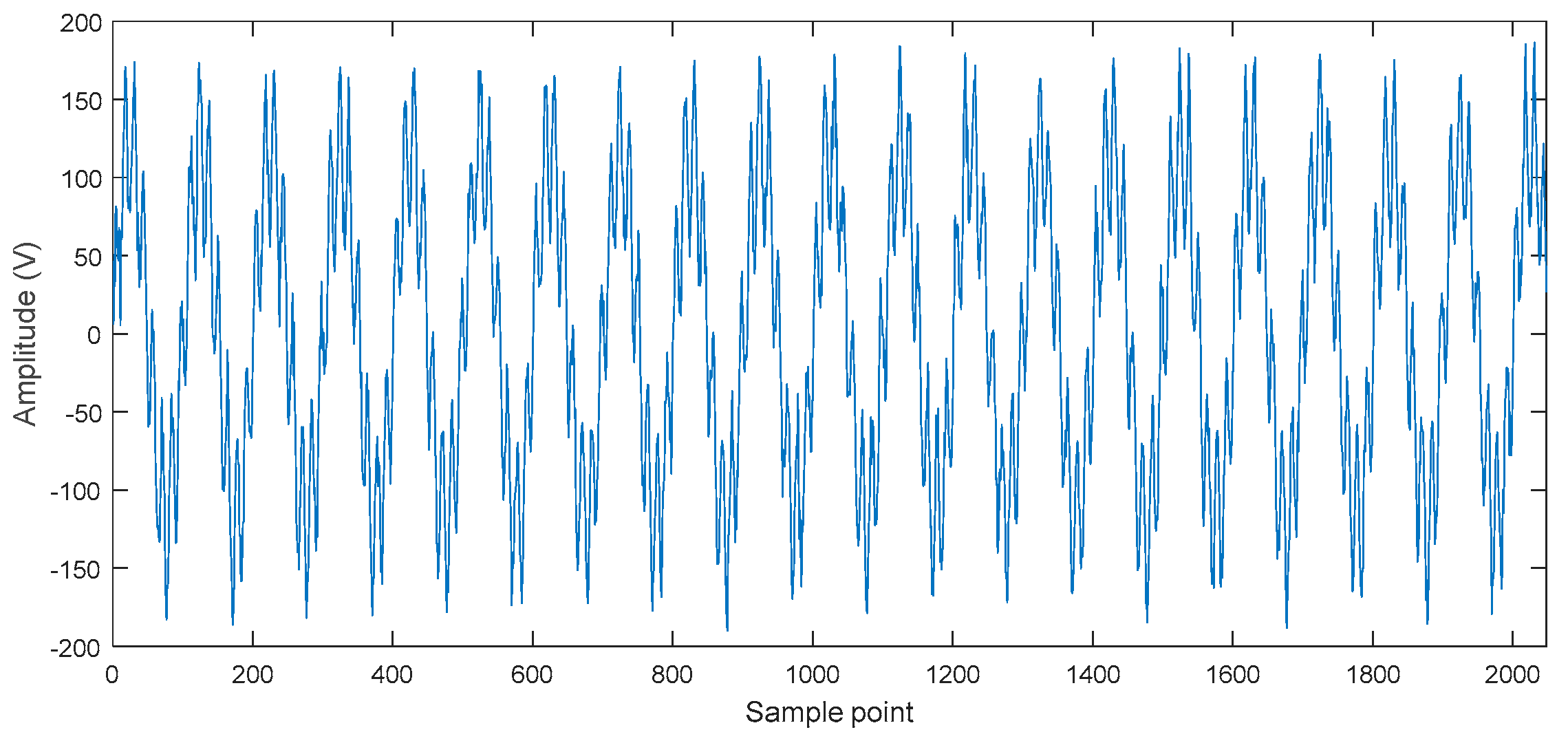
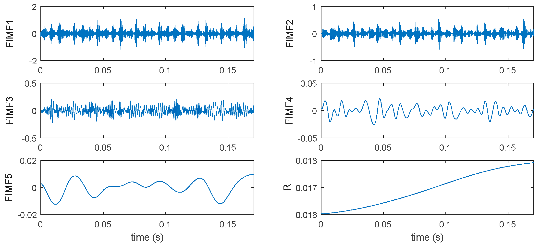
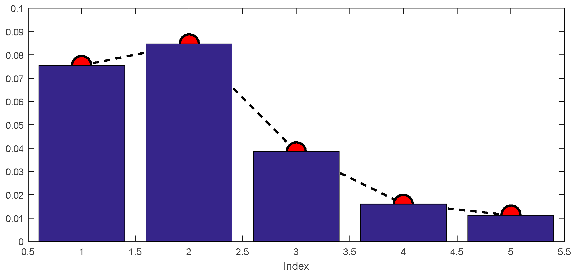
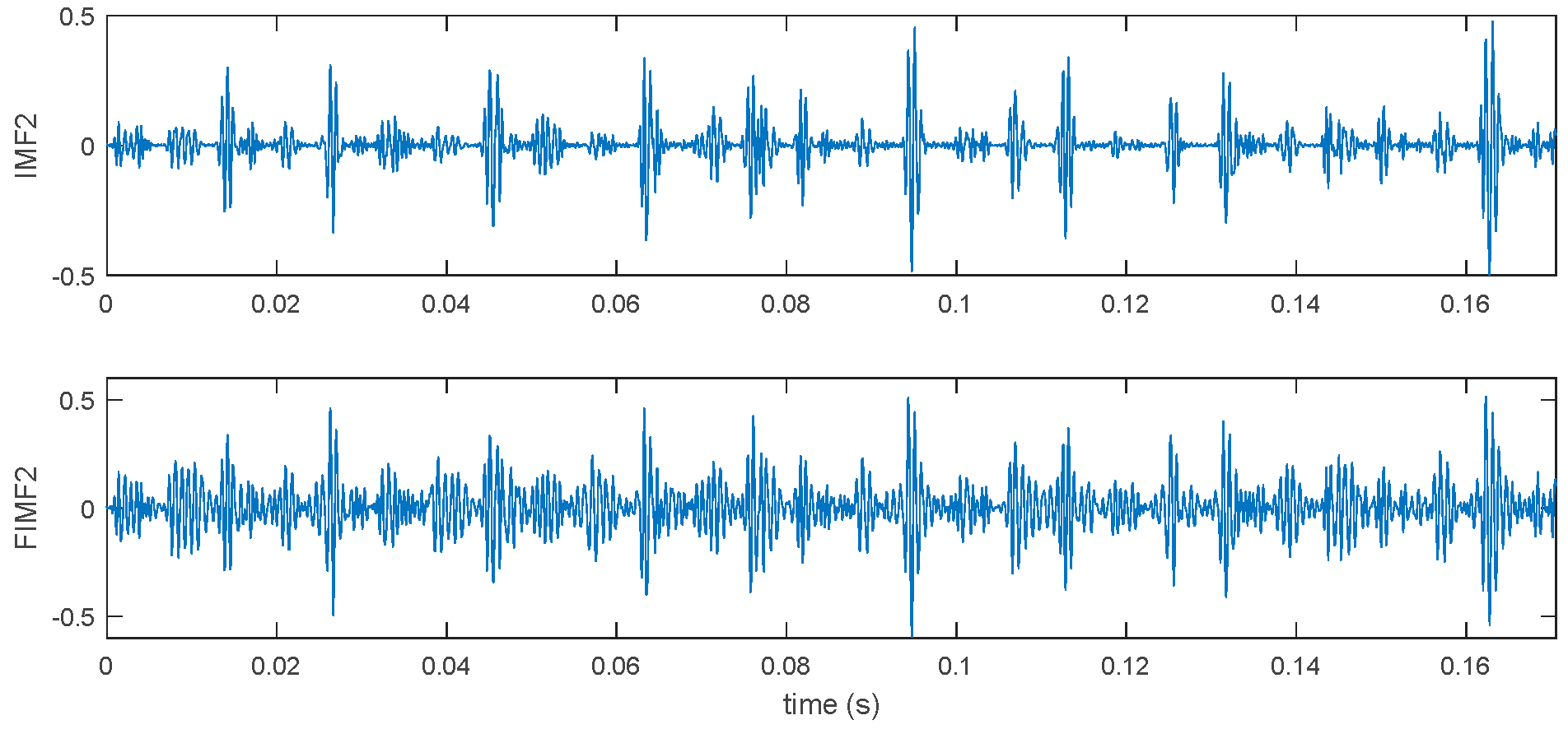
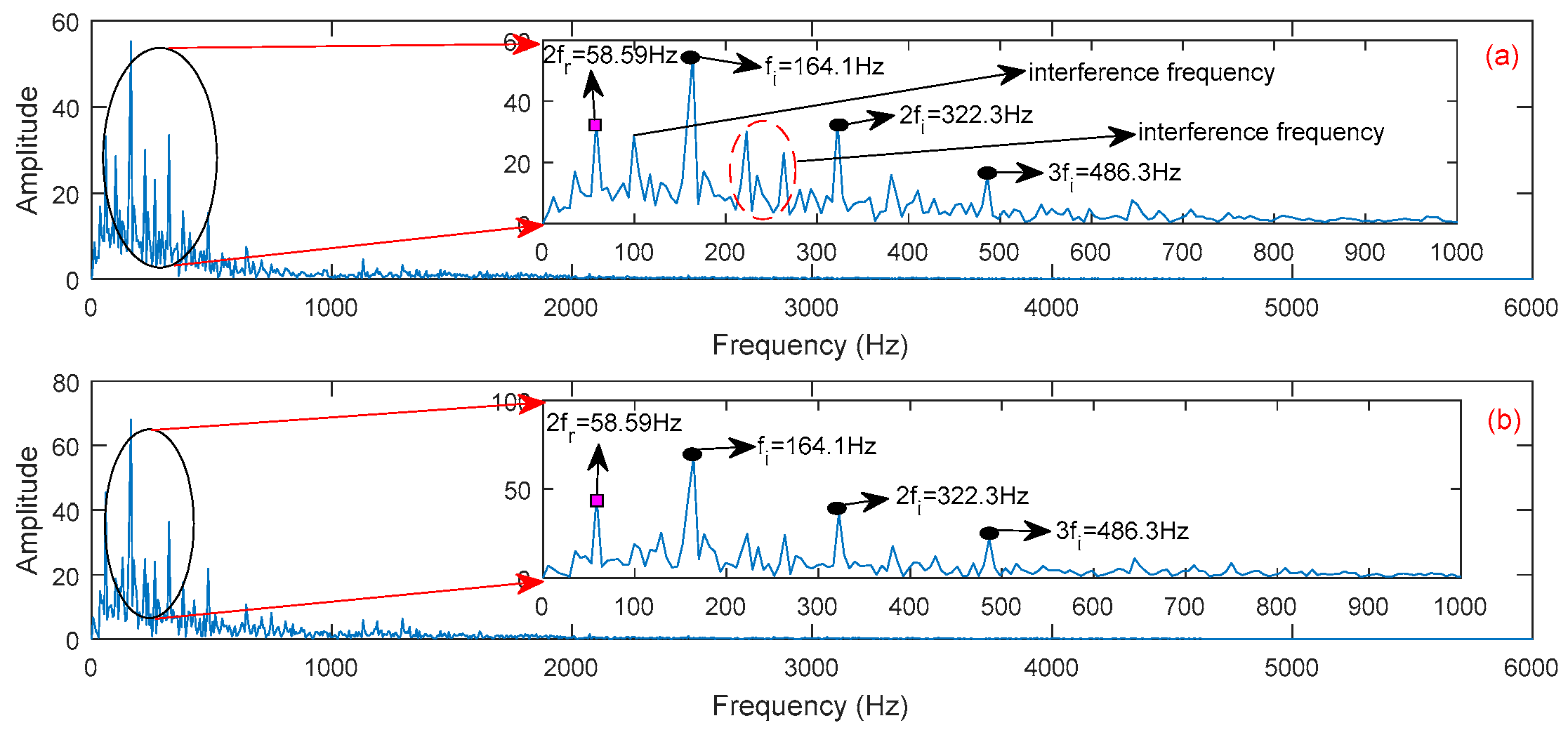
4.1. Diagnose Inner Raceway Fault of Rolling Bearing

In this section, the proposed method is applied to identify the feature frequencies of fault signal, which draws upon the website of the Case Western Reserve University [52], to illustrate its performance. The experiment rig consisted of a 2 HP motor, a torque transducer, a dynamometer and control electronics (as shown Figure 10).

Table 1. Bearing parameter of 6205-2RS deep groove ball bearing.

Bearing Type	$\mathbf{Ball}\mathbf{Number}\mathit{n}$	$\mathbf{Pitch}\mathbf{Diameter}\mathit{D}$ (mm)	$\mathbf{Ball}\mathbf{Diameter}\mathit{d}$ (mm)	$\mathbf{Contact}\mathbf{Angle}\mathit{\alpha }$ (°)
6205-2RS	9	52	8	0

presents the parameters of the rolling bearing (bearings type: 6205-2RS SKF deep groove ball).

The following equation is the theoretical feature frequency of inner raceway fault ($f_{in}$).

$$f_{in}=0.5n\left(1+\frac{d}{D}cos\alpha \right)f_r$$

(20)

Here, $f_r$ is the rotation frequency.

The test bearing presented a single point fault with fault diameters of 0.018 mm by electro-discharge machining. The sample rate was 12 kHz. The experiment data was selected from the drive end and motor load 0 (HP), and the motor speed was 1797 RPM. The data length was 2048 (as shown in Figure 11).

Here, CEEMDAN is used to decompose the vibration signal (ensemble size is 100, and the amplitude of the added noise is 0.2). The eleven IMFs and one residue were obtained (as shown Figure 12). It was found that it does not reflect the real component of original signal for each IMF completely, and that it contains some spurious information (such as IMF₁₀). To extract the IIM of the vibration signal, the CIMFs were first obtained using Equation (16), and then FFT and the corresponding local zoom (main information) were conducted for each CIMF (as shown in Figure 13). It was found by comparing FC1 with FC2 that there were additional frequency bands. Similarly, the frequency component in FC6 is different from that of FC7 (the detail difference is shown Figure 14). That in FC8 is also different from that in FC9; this means that the feature difference is easy to distinguished among IMFs using the proposed method.

The MHD is used to calculate the similar of adjacent PCs. If they are similar, the MHD is relatively small and vice versa. Figure 15 is the MHD of adjacent FCs. It is found that the theoretical cut-off point in Figure 13 is originally the third and sixth point. However, the MHD does not reflect the local maximum; it illustrates that when the MHD calculates the similarity of adjacent FCs directly, the difference of frequency features is not identified.

To identify the cut-off point of FCs, the PDF of each FC is estimated by the normal Kernel density function. Meanwhile, the MHD is also used to calculate similar of adjacent PFCs (as shown in Figure 16).

It was found that there are four local maxima points. The Figure 17 is the relational graph among the CIMFs; this illustrates that CIMF₁ is not similar to CIMF₂, CIMF₃ is not similar to CIMF₄, CIMF₆ is not similar to CIMF₇, CIMF₈ is not similar with CIMF₉, and the residues are similar.

Thus, five FIMFs are obtained using the proposed method (as shown in Equation (21)). Figure 18 presents the FIMFs and residue.

$$\begin{array}{l}{\mathrm{FIMF}}_1{=\mathrm{IMF}}_1\\ {\mathrm{FIMF}}_2{=\mathrm{IMF}}_2{+\mathrm{IMF}}_3\\ {\mathrm{FIMF}}_3{=\mathrm{IMF}}_4{+\mathrm{IMF}}_5{+\mathrm{IMF}}_6\\ {\mathrm{FIMF}}_4{=\mathrm{IMF}}_7{+\mathrm{IMF}}_8\\ {\mathrm{FIMF}}_5{=\mathrm{IMF}}_9{+\mathrm{IMF}}_{10}{+\mathrm{IMF}}_{11}\end{array}$$

(21)

Next, the method in Section 3.2 was used to identify IIM (scales range of DFA is from 10 to 100 with step 5). Figure 19 is the comprehensive evaluated index. It was found that the biggest value is the $S_2$ of the FIMF₂; this illustrates that FIMF₂ should be used to extract fault information from the vibration signal. Meanwhile, to compare performance of proposed method, the original CEEMDAN, combined with comprehensive evaluated index, is also used to extract fault information for rolling bearings (as shown in Figure 20). It was found that the second point was the maximum point; this means that the IMF₂ contains the main fault features of vibration signal. Figure 21 shows the identified IMF2 and FIMF2.

Finally, the envelope spectrum was used to identify the frequency components of IMF₂ and FIMF₂ (as shown in Figure 22a,b). It was found that $2f_r$,$f_i$,$2f_i$,$3f_i$ are all identified for IMF₂ and FIMF₂. The envelope spectrum of FIMF₂ does not contain any interference frequency. However, that of IMF₂ abundantly contains the interference frequency; this means that the proposed method can effectively identify fault information of rolling bearings. Meanwhile, the original signal was also used for the envelope spectrum (as shown in Figure 23). It was found that there is a greater interference component compared to IMF2. In addition, the computational load of the proposed method is compared with CEEMDAN; they are 20.24 s and 19.26 s, respectively (the amplitude of added white noise and ensemble trails are 0.1 and 100, respectively). There was only a difference of 0.98 s (the used laptop has Core i5-3230M CPU, 2.60 Ghz, RAM is 6 GB). However, the decomposed effectiveness for proposed method outperformed that of CEEMDAN. Thus, the proposed method is more suitable for fault diagnoses of rolling bearings.

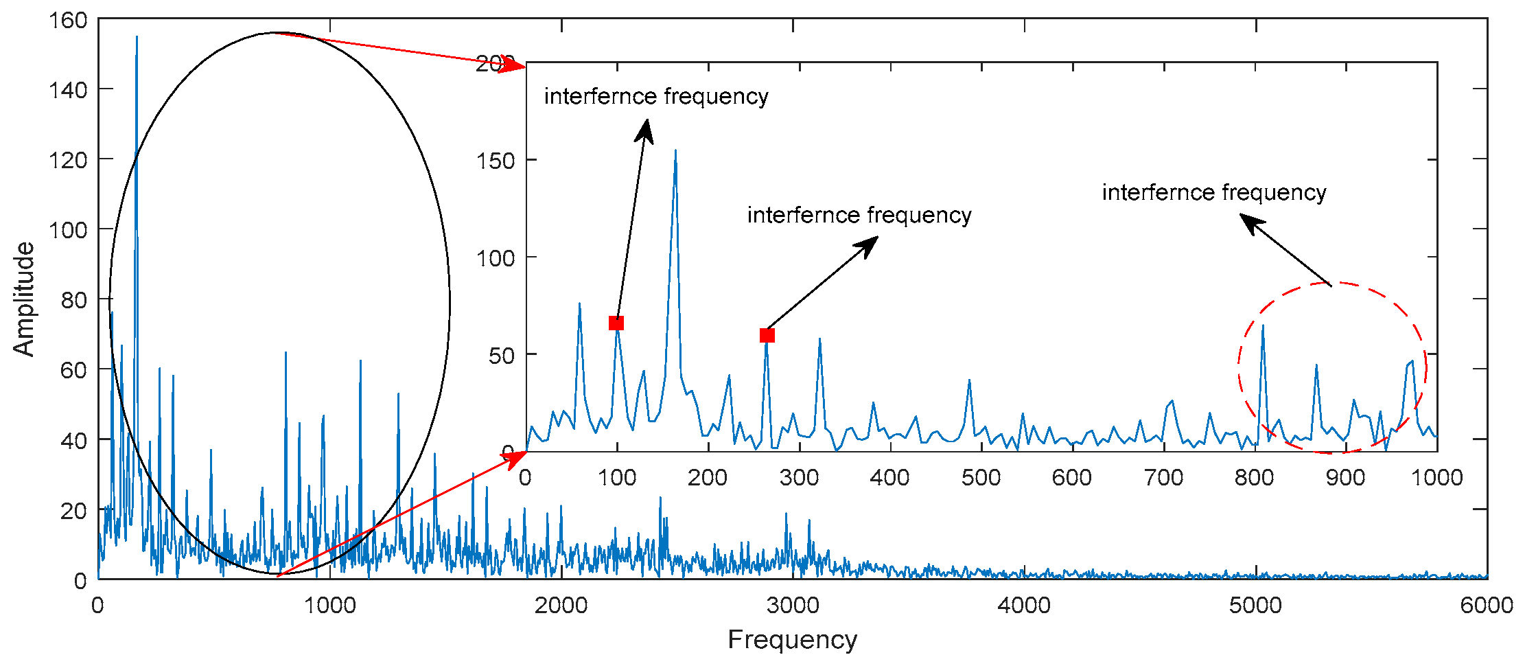
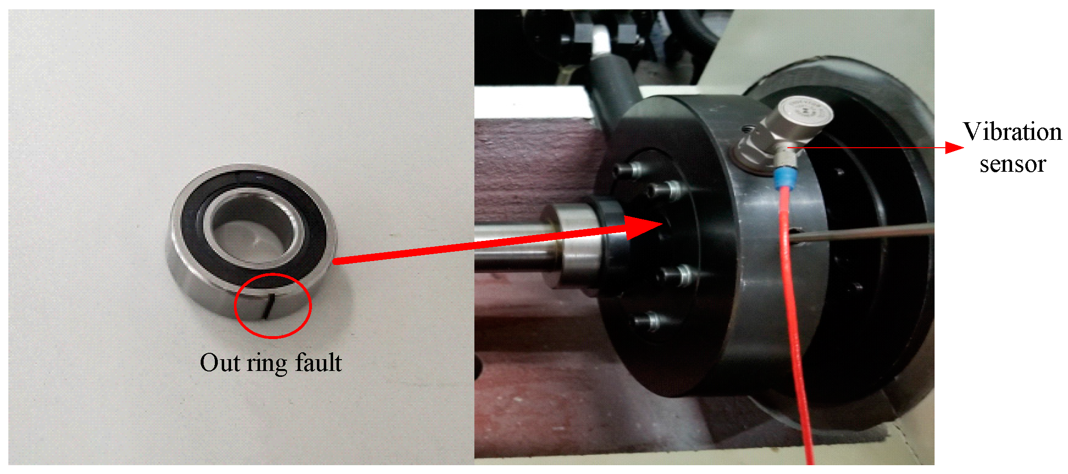
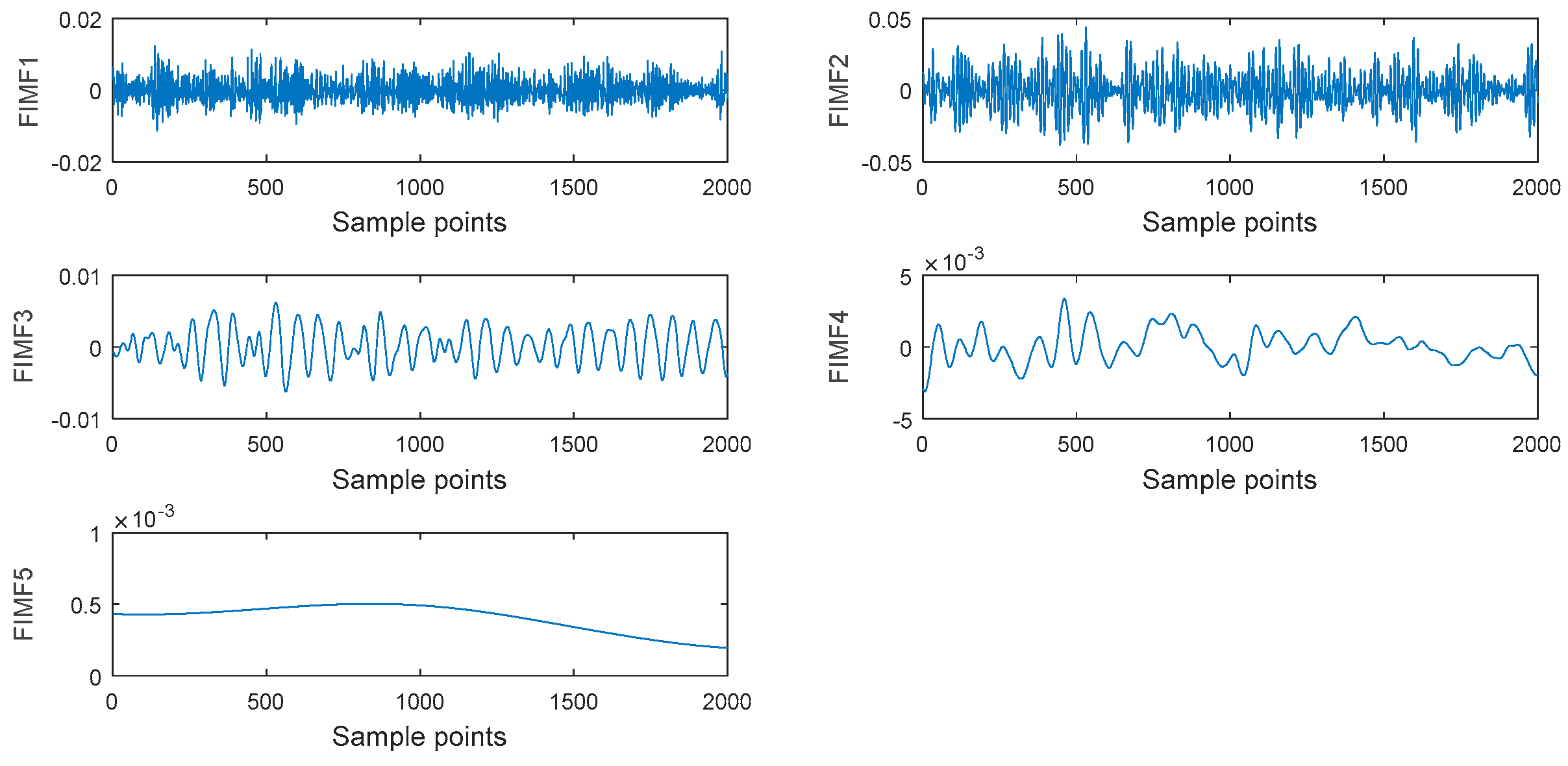
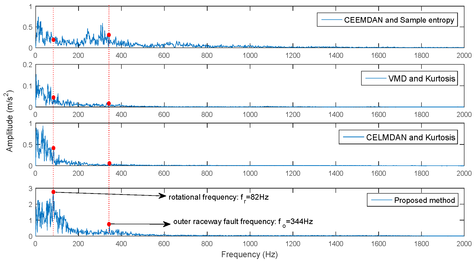
4.2. Diagnose Outer Raceway Fault of Rolling Bearing

In this experiment, the following setup (as shown in Figure 24) was used to extract the fault features of rolling bearings. It consisted of four rolling bearings (symbols 1–4), an electric spindle (symbol 5), four temperature sensors (for monitoring the temperature of the bearing out ring; symbol 6), two non-contact temperature sensors (for monitoring the temperature of the inner raceway; symbol 7), and a load cell (symbol 8).

The test bearing presented a single point fault which was caused by electro-discharge machining (as shown in Figure 25).

Table 2. Bearing parameters in this experiment.

$\mathbf{Ball}\mathbf{Number}\mathit{n}$	$\mathbf{Pitch}\mathbf{Diameter}\mathit{D}$ (mm)	$\mathbf{Ball}\mathbf{Diameter}\mathit{d}$ (mm)	$\mathbf{Contact}\mathbf{Angle}\mathit{\alpha }$ (°)
10	46	7.9	0

shows the bearing parameters.

Equation (22) is the theoretical feature frequency of the outer raceway fault ($f_{\mathrm{o}}$):

$$f_{in}=0.5n\left(1-\frac{d}{D}cos\alpha \right)f_r$$

(22)

The sample rate was 4 kHz. The selected data length was 2000 (as shown in Figure 26).

Firstly, the proposed method was used to obtain FIMFs. The two critical parameters in CEEMDAN were 0.2 (the amplitude of added white noise) and 100 (ensemble size). FIMFs are shown in Figure 27. Then, the comprehensive evaluated index was used to identify the IIM (scales range of DFA was from 10 to 100, with step 5 in this paper). Meanwhile, the AE, SE and FE were also used to identify IIM to compare the identified performance with the proposed method. Figure 28 is the identified result. It was found that the second FIMF is IIM for AE, FE and the proposed method. However, the difference in values between the first and second FIMFs for the proposed method is more obvious than in the other methods (the corresponding ratios are 1.01, 1.02 and 1.21 for the three kinds of method); this proves that the proposed method has a strong ability to identify faults, relative to the AE and FE methods. The envelope spectrum was conducted for the second FIMF to extract fault information. Meanwhile, to compare the extracted ability of the rolling bearing, the first FIMF identified by the SE method, VMD [53] and CELMDAN combining with kurtosis [24] were employed to extract fault information. Figure 29a,b shows the kurtosis for the VMD and CELMDAN methods. It was found that the largest value was the index of the forth IMF and the second PF. Figure 30 is the corresponding envelope spectrum. It shows that the feature frequency (rotational frequency ($f_r=82\mathrm{Hz}$) and the outer raceway fault frequency ($f_{\mathrm{o}}=344\mathrm{Hz}$)) were more obvious than those obtained using the other methods. Here, the theoretical $f_r$ and $f_{\mathrm{o}}$ are 83.33 Hz and 344.76 Hz, as obtained by Equation (22) (the rotational speed is 9000R/min), respectively. The corresponding amplitude is bigger than the others methods. However, for the AE, VMD and CELMDAN methods, it was very difficult to extract rotational speeds and fault frequencies; this is because the extra information interferes with the normal vibration signal, and the rotational frequency and outer raceway fault frequency were all submerged. Thus, it also indicates that the proposed method is more effective at extracting faults in the outer raceways of rolling bearings.

5. Conclusions

This paper develops a novel method to extract the feature frequencies of rolling bearing. Figure 31 is a flowchart of diagnosis process. The following conclusions may be drawn:

(1)

Our research introduces a method which combines adjacent IMFs into a novel mode function (CIMF) to enhance difference characteristics among IMFs (as shown in step 2).

(2)

It proposes a method of combing FFT, PDF and MHD to obtain final intrinsic information mode (FIMF) of minimum number and with physical meanings (as shown in step 3).

(3)

It introduces a comprehensive evaluate index (DFA and Kurtosis) to identify intrinsic information mode (IIM) to extract the feature frequencies of rolling bearings (as shown in step 4).

The experiment results indicate that this method can minimize interference of spurious mode in original CEEMDAN decomposition, and that it can accurately extract information. Furthermore, the method is also compared with some typical methods. The results indicate that the proposed method has remarkable advantages for the extraction of fault features of rolling bearings.

References

1. Zhao, S.; Liang, L.; Xu, G.; Wang, J.; Zhang, W. Quantitative diagnosis of a spall-like fault of a rolling element bearing by empirical mode decomposition and the approximate entropy method. Mech. Syst. Signal Process. 2013, 40, 154–177. [Google Scholar] [CrossRef]
2. Yang, H.; Mathew, J.; Ma, L. Fault diagnosis of rolling element bearings using basis pursuit. Mech. Syst. Signal Process. 2005, 19, 341–356. [Google Scholar] [CrossRef]
3. Kang, M.; Kim, J.; Kim, J.-M.; Tan, A.C.C.; Kim, E.Y.; Choi, B.-K.; Kim, J. Reliable Fault Diagnosis for Low-Speed Bearings Using Individually Trained Support Vector Machines With Kernel Discriminative Feature Analysis. Power Electron. IEEE Trans. 2015, 30, 2786–2797. [Google Scholar] [CrossRef] [Green Version]
4. Bluestein, L.I. A linear filtering approach to the computation of discrete Fourier transform. Audio Electroacoust. IEEE Trans. 1970, 18, 451–455. [Google Scholar] [CrossRef]
5. Wang, T.; Lin, J. Fault Diagnosis of Rolling Bearings Based on Wavelet Packet and Spectral Kurtosis. In Proceedings of the Fourth International Conference on Intelligent Computation Technology and Automation, Guangdong, China, 28–29 March 2011; pp. 665–669. [Google Scholar]
6. Wang, J.; He, Q. Wavelet Packet Envelope Manifold for Fault Diagnosis of Rolling Element Bearings. IEEE Trans. Instrum. Meas. 2016, 65, 2515–2526. [Google Scholar] [CrossRef]
7. Huang, N.E.; Shen, Z.; Long, S.R.; Wu, M.C.; Shih, H.H.; Zheng, Q.; Yen, N.-C.; Tung, C.C.; Liu, H.H. The empirical mode decomposition and the Hilbert spectrum for nonlinear and non-stationary time series analysis. Proc. Math. Phys. Eng. Sci. 1998, 454, 903–995. [Google Scholar]
8. Pittman-Polletta, B.; Hsieh, W.H.; Kaur, S.; Lo, M.T.; Hu, K. Detecting phase-amplitude coupling with high frequency resolution using adaptive decompositions. J. Neurosci. Methods 2014, 226, 15–32. [Google Scholar] [CrossRef] [Green Version]
9. Yeh, C.H.; Lo, M.T.; Hu, K. Spurious cross-frequency amplitude-amplitude coupling in nonstationary, nonlinear signals. Phys. A Stat. Mech. Its Appl. 2016, 454, 143–150. [Google Scholar] [Green Version]
10. Yeh, C.H.; Shi, W. Identifying Phase-Amplitude Coupling in Cyclic Alternating Pattern using Masking Signals. Sci. Rep. 2018, 8, 2649. [Google Scholar] [Green Version]
11. Deering, R.; Kaiser, J.F. The use of a masking signal to improve empirical mode decomposition. In Proceedings of the IEEE International Conference on Acoustics, Speech, and Signal Processing, Philadelphia, PA, USA, 23–23 March 2005. [Google Scholar]
12. Wu, Z.; Huang, N.E. Ensemble Empirical Mode Decomposition: A Noise-Assissted Data Analysis Method. Adv. Adapt. Data Anal. 2011, 1, 1–41. [Google Scholar]
13. Yeh, J.-R.; Shieh, J.-S.; Huang, N.E. Complementary ensemble empirical mode decomposition: A novel noise enhanced data analysis method. Adv. Adapt. Data Anal. 2010, 2, 135–156. [Google Scholar] [CrossRef]
14. Torres, M.E.; Colominas, M.A.; Schlotthauer, G.; Flandrin, P. A complete ensemble empirical mode decomposition with adaptive noise. In Proceedings of the IEEE International Conference on Acoustics, Speech and Signal Processing, Prague, Czech Republic, 22–27 May 2011; pp. 4144–4147. [Google Scholar]
15. Lei, Y.; He, Z.; Zi, Y. Application of the EEMD method to rotor fault diagnosis of rotating machinery. Mech. Syst. Signal Process. 2009, 23, 1327–1338. [Google Scholar] [CrossRef]
16. Lei, Y.; Zuo, M.J. Fault diagnosis of rotating machinery using an improved HHT based on EEMD and sensitive IMFs. Meas. Sci. Technol. 2009, 20, 125701. [Google Scholar] [CrossRef]
17. Zhou, Y.; Tao, T.; Mei, X.; Jiang, G.; Sun, N. Feed-axis gearbox condition monitoring using built-in position sensors and EEMD method. Robot. Comput.-Integr. Manuf. 2011, 27, 785–793. [Google Scholar] [CrossRef]
18. Chang, K.M.; Liu, S.H. Gaussian Noise Filtering from ECG by Wiener Filter and Ensemble Empirical Mode Decomposition. J. Signal Process. Syst. 2011, 64, 249–264. [Google Scholar] [CrossRef]
19. Zhang, J.; Yan, R.; Gao, R.X.; Feng, Z. Performance enhancement of ensemble empirical mode decomposition. Mech. Syst. Signal Process. 2010, 24, 2104–2123. [Google Scholar]
20. Žvokelj, M.; Zupan, S.; Prebil, I. Non-linear multivariate and multiscale monitoring and signal denoising strategy using Kernel Principal Component Analysis combined with Ensemble Empirical Mode Decomposition method. Mech. Syst. Signal Process. 2011, 25, 2631–2653. [Google Scholar]
21. Žvokelj, M.; Zupan, S.; Prebil, I. Multivariate and multiscale monitoring of large-size low-speed bearings using Ensemble Empirical Mode Decomposition method combined with Principal Component Analysis. Mech. Syst. Signal Process. 2010, 24, 1049–1067. [Google Scholar]
22. Colominas, M.A.; Schlotthauer, G.; Torres, M.E. Improved complete ensemble EMD: A suitable tool for biomedical signal processing. Biomed. Signal Process. Control 2014, 14, 19–29. [Google Scholar]
23. Yang, Y.; Cheng, J.; Zhang, K. An ensemble local means decomposition method and its application to local rub-impact fault diagnosis of the rotor systems. Measurement 2012, 45, 561–570. [Google Scholar] [CrossRef]
24. Wang, L.; Liu, Z.; Miao, Q.; Zhang, X. Complete ensemble local mean decomposition with adaptive noise and its application to fault diagnosis for rolling bearings. Mech. Syst. Signal Process. 2018, 106, 24–39. [Google Scholar] [CrossRef]
25. Gao, Q.; Duan, C.; Fan, H.; Meng, Q. Rotating machine fault diagnosis using empirical mode decomposition. Mech. Syst. Signal Process. 2008, 22, 1072–1081. [Google Scholar] [CrossRef]
26. Laha, S.K. Enhancement of fault diagnosis of rolling element bearing using maximum kurtosis fast nonlocal means denoising. Measurement 2017, 100, 157–163. [Google Scholar]
27. Cheng, J.; Ma, X.; Yang, Y. The Rolling Bearing Fault Diagnosis Method Based on Correlation Coefficient of Independent Component Analysis and VPMCD. J. Vib. Meas. Diagn. 2015, 35, 645–648. [Google Scholar]
28. Jin, P.; Wang, W.; Wang, H.; Tang, X. Fault diagnosis method of wind turbine’s bearing based on EEMD kurtosis-correlation coefficients criterion and multiple features. Renew. Energy Resour. 2016, 34, 1481–1490. [Google Scholar]
29. Harmouche, J.; Delpha, C.; Diallo, D. Faults diagnosis and detection using principal component analysis and Kullback-Leibler divergence. In Proceedings of the Conference of the IEEE Industrial Electronics Society, Montreal, QC, Canada, 25–28 October 2012. [Google Scholar]
30. Woo, W.; Gao, B.; Bouridane, A.; Ling, B.; Chin, C. Unsupervised Learning for Monaural Source Separation Using Maximization–Minimization Algorithm with Time–Frequency Deconvolution. Sensors 2018, 18, 1371. [Google Scholar] [CrossRef]
31. Zhang, F.; Liu, Y.; Chen, C.; Li, Y.F.; Huang, H.Z. Fault diagnosis of rotating machinery based on kernel density estimation and Kullback-Leibler divergence. J. Mech. Sci. Technol. 2014, 28, 4441–4454. [Google Scholar]
32. Shang, D.; Xu, M.; Shang, P. Generalized sample entropy analysis for traffic signals based on similarity measure. Phys. A Stat. Mech. Its Appl. 2017, 474, 1–7. [Google Scholar]
33. Deng, F.; Tang, G. An intelligent method for rolling element bearing fault diagnosis based on time-wavelet energy spectrum sample entropy. J. Vib. Shock 2017, 36, 28–34. [Google Scholar]
34. Yan, R.; Gao, R.X. Approximate Entropy as a diagnostic tool for machine health monitoring. Mech. Syst. Signal Process. 2007, 21, 824–839. [Google Scholar] [CrossRef]
35. Li, X.; He, N.; He, K. Cylindrical Roller Bearing Diagnosis Based on Wavelet Packet Approximate Entropy and Support Vector Machines. J. Vib. Meas. Diagn. 2015, 35, 1031–1036. [Google Scholar]
36. Luukka, P. Feature selection using fuzzy entropy measures with similarity classifier. Expert Syst. Appl. 2011, 38, 4600–4607. [Google Scholar] [CrossRef]
37. Chen, W.; Wang, Z.; Xie, H.; Yu, W. Characterization of Surface EMG Signal Based on Fuzzy Entropy. IEEE Trans. Neural Syst. Rehabil. Eng. 2007, 15, 266–272. [Google Scholar] [CrossRef]
38. Cerrada, M.; Ren, S. A review on data-driven fault severity assessment in rolling bearings. Mech. Syst. Signal Process. 2018, 99, 169–196. [Google Scholar]
39. Gao, Z.; Cecati, C.; Ding, S.X. A Survey of Fault Diagnosis and Fault-Tolerant Techniques—Part I: Fault Diagnosis With Model-Based and Signal-Based Approaches. IEEE Trans. Ind. Electron. 2015, 62, 3757–3767. [Google Scholar] [Green Version]
40. Nguyen, T.L.; Djeziri, M.; Ananou, B.; Ouladsine, M.; Pinaton, J. Fault prognosis for batch production based on percentile measure and gamma process: Application to semiconductor manufacturing. J. Process Control 2016, 48, 72–80. [Google Scholar]
41. Benmoussa, S.; Djeziri, M.A. Remaining useful life estimation without needing for prior knowledge of the degradation features. IET Sci. Meas. Technol. 2017, 11, 1071–1078. [Google Scholar]
42. Li, H.; Liu, T.; Wu, X.; Chen, Q. Application of EEMD and improved frequency band entropy in bearing fault feature extraction. ISA Trans. 2018. [Google Scholar] [CrossRef]
43. Dubuisson, M.P.; Jain, A.K. A modified Hausdorff distance for object matching. In Proceedings of the International Conference on Pattern Recognition, Jerusalem, Israel, 9–13 October 2002; Volume 1, pp. 566–568. [Google Scholar]
44. Chen, Z.; Hu, K.; Carpena, P.; Bernaola-Galván, P.; Stanley, H.E.; Ivanov, P.C. Effect of nonlinear filters on detrended fluctuation analysis. Phy. Rev. E 2005, 71, 011104. [Google Scholar] [CrossRef]
45. Chen, Z.; Ivanov, P.C.; Hu, K.; Stanley, H.E. Effect of nonstationarities on detrended fluctuation analysis. Phys. Rev. E 2002, 65, 041107. [Google Scholar] [CrossRef]
46. Horvatic, D.; Stanley, H.E.; Podobnik, B. Detrended cross-correlation analysis for non-stationary time series with periodic trends. Europhys. Lett. 2011, 94, 18007. [Google Scholar] [CrossRef]
47. Lv, Y.; Yuan, R.; Wang, T.; Li, H.; Song, G. Health Degradation Monitoring and Early Fault Diagnosis of a Rolling Bearing Based on CEEMDAN and Improved MMSE. Materials 2018, 11, 1009. [Google Scholar]
48. Bouhalais, M.L.; Djebala, A.; Ouelaa, N.; Babouri, M.K. CEEMDAN and OWMRA as a hybrid method for rolling bearing fault diagnosis under variable speed. Int. J. Adv. Manuf. Technol. 2017, 94, 2475–2489. [Google Scholar] [CrossRef]
49. Huttenlocher, D.P.; Klanderman, G.; Rucklidge, W.J. Comparing images using the Hausdorff distance. IEEE Trans. Pattern Anal. Mach. Intell. 1993, 15, 850–863. [Google Scholar]
50. Zhao, C.; Shi, W.; Deng, Y. A New Hausdorff Distance for Image Matching; Elsevier Science Inc.: New York, NY, USA, 2005. [Google Scholar]
51. Schutze, O.; Esquivel, X.; Lara, A.; Coello, C.A.C. Using the Averaged Hausdorff Distance as a Performance Measure in Evolutionary Multiobjective Optimization. IEEE Trans. Evol. Comput. 2012, 16, 504–522. [Google Scholar]
52. Loparo, K.A. Bearing Data Center. Case Western Reserve University, 2000. Available online: http://csegroups.case.edu/bearingdatacenter/home (accessed on 10 February 2019).
53. Zhao, H.; Li, L. Fault diagnosis of wind turbine bearing based on variational mode decomposition and Teager energy operator. IET Renew. Power Gener. 2016, 11, 453–460. [Google Scholar] [CrossRef]
Figure 1. Simulated signal.
Symmetry 11 00513 g001
Figure 2. Decomposition of simulated signal by CEEMDAN.
Symmetry 11 00513 g002
Figure 3. Combined IMF.
Symmetry 11 00513 g003
Figure 4. FFT of CIMF.
Symmetry 11 00513 g004
Figure 5. PDF of CMF.
Symmetry 11 00513 g005
Figure 6. Calculated result of MHD.
Symmetry 11 00513 g006
Figure 7. Relational graph of CIMF.
Symmetry 11 00513 g007
Figure 8. FIMF and corresponding frequency.
Symmetry 11 00513 g008
Figure 9. Flow chart of proposed method.
Symmetry 11 00513 g009
Figure 10. Experiment rig of rolling bearings [52].
Symmetry 11 00513 g010
Figure 11. Vibration signal of bearing fault.
Symmetry 11 00513 g011
Figure 12. Decomposed result of vibration signal by CEEMDAN.
Symmetry 11 00513 g012
Figure 13. FFT of each CIMF.
Symmetry 11 00513 g013
Figure 14. Detail difference of frequency component between FC6 and FC7.
Symmetry 11 00513 g014
Figure 15. MHD of each FC.
Symmetry 11 00513 g015
Figure 16. MHD of each PFC.
Symmetry 11 00513 g016
Figure 17. Relational graph among the CIMFs.
Symmetry 11 00513 g017
Figure 18. FIMF obtained by proposed method.
Symmetry 11 00513 g018
Figure 19. Identified result of FIMF.
Symmetry 11 00513 g019
Figure 20. Identified result of IMF.
Symmetry 11 00513 g020
Figure 21. IMF2 and FIMF2.
Symmetry 11 00513 g021
Figure 22. (a) Envelope spectrum of IMF2; (b) Envelope spectrum of FIMF2.
Symmetry 11 00513 g022
Figure 23. Envelope spectrum of original signal.
Symmetry 11 00513 g023
Figure 24. Experiment setup of rolling bearing.
Symmetry 11 00513 g024
Figure 25. Bearings with outer raceway fault and corresponding housing.
Symmetry 11 00513 g025
Figure 26. Fault signal of outer raceway fault of rolling bearing.
Symmetry 11 00513 g026
Figure 27. Obtained final intrinsic mode function.
Symmetry 11 00513 g027
Figure 28. Comparison of identified IIM with AE, SE, FE and the proposed method.
Symmetry 11 00513 g028
Figure 29. (a) Identifying of IIM with kurtosis method for IMF; (b) Identifying of IIM with kurtosis method for PF.
Symmetry 11 00513 g029
Figure 30. Comparison of feature frequencies for different methods.
Symmetry 11 00513 g030
Figure 31. Flowchart of fault diagnosis for rolling bearing.
Symmetry 11 00513 g031