Abstract
As a subject area of symmetry, multiple instance learning (MIL) is a special form of a weakly supervised learning problem where the label is related to the bag, not the instances contained in it. The difficulty of MIL lies in the incomplete label information of instances. To resolve this problem, in this paper, we propose a novel diverse density (DD) and multiple part similarity combination method for multiple instance learning, named MILDMS. First, we model the target concepts optimization with a DD function constraint on positive and negative instance space, which can greatly improve the robustness to label noise problem. Next, we combine the positive and negative instances in the bag (generated by hand-crafted and convolutional neural network features) with multiple part similarities to construct an MIL kernel. We evaluate the proposed approach on the MUSK dataset, whose results MUSK1 (91.9%) and MUSK2 (92.2%) show our method is comparable to other MIL algorithms. To further demonstrate generality, we also present experimental results on the PASCAL VOC 2007 and 2012 (46.5% and 42.2%) and COREL (78.6%) that significantly outperforms the state-of-the-art algorithms including deep MIL and other non-deep MIL algorithms.
1. Introduction
Multiple instance learning (MIL), i.e., learning from ambiguous data (the labels are related to bags, not instances within the bags, meaning that we only have partial or incomplete knowledge about training instances), has been widely studied and applied to many challenging tasks, such as text categorization [1], object tracking [2], person re-identification [3], computer-aided medical diagnosis [4], etc. Therefore, it has received considerable attention, and various algorithms, for example APR [5], DD [6], Citation-KNN [7], EM-DD [8], MI-Kernel [9], miSVM and MISVM [10], DD-SVM [11], MILES [12], MissSVM [13], MIGraph and miGraph [14], MILIS [15], MILDS [16], MILEAGE [17], mi-DS [18], CK_MIL [19], SMILE [20], MIKI [21], TreeMIL [22], MILDM [23], mi-Net and MI-Net [24], Attention and Gated-Attention MIL [25], etc., have been proposed to deal with the MIL problem. However, there are two issues that hinder its practical application. One is that most of these methods are sensitive to noise, which makes the mislabeled labels degrade the classification performance. The other is that these methods cannot deal well with both one target concept and multiple target concepts problems in one MIL framework. In this paper, we combine a novel diverse density (DD) constraint optimization model with multiple part similarity, named MILDMS, to handle the above two MIL issues by using hand-crafted and deep features in image categorization.
As an important paradigm in machine learning, the MIL was firstly proposed by Dietterich [5] in the context of drug activity prediction task, where a drug molecule is suitable for drug design if one of its conformations can tightly bind to the protein molecules, but the biochemical data can only tell us the binding capability of drug molecule, not its particular conformations. In MIL, to facilitate expression, the drug molecule and its conformations are named bag and instances separately. In this learning scheme, rather than representing each training bag as a fixed-length vector, each bag contains a set of instances (different size fixed-length vectors).
Under the MIL assumption, all the instances in negative bags are negative, whereas instances in positive bag are either positive or negative instances. Thus, the intuition MIL algorithms, such as APR [5] and DD [6], attempt to find a dense positive instance rectangle or ellipse region (also named as target concept region) in instance space, which can be seen as an intersection of positive bags, by expanding or shrinking axis-parallel rectangle (APR) or optimizing a DD function. The experimental results on drug activity prediction have proven the performance of these two algorithms. Unfortunately, both of APR and DD are sensitive to noise because the noise data will greatly change the rectangle of APR and influence the DD value. Moreover, the APR and DD cannot capture the multiple target concepts in many MIL real-world applications, such as image categorization, image retrieval, etc.
For the image categorization problem, it can be naturally casted as multiple instance learning by treating the image as the bag and segmented regions of it as instances. Unlike the drug activity prediction, the image categorization is collectively determined by parts of instances (segmented regions) of the bag (image) or even all these instances. For example, the image labeled as ‘africa’ should contain not only people, but also elephants, savannah, lions, etc., because the high-level semantic ‘africa’ is determined by these objects.
Noting that the multiple target concepts problem existed in image categorization and the difficulty caused by it, Chen advocates to seek multiple DD points in instance space and convert the image (bag) to fixed-length features [11]. Unfortunately, this method is also sensitive to noise. To overcome this problem, Chen consequently proposes another algorithm named MILES [12], which maps the bag to a very high space generated by all instances of training bags and uses 1-norm SVM to select the target concepts. The shortcoming of this method is that the mapping process has high computation complexity.
In this paper, we propose a novel MIL method named MILDMS, which introduces an indicator vector for each instance and models the target concepts optimization process with a DD function constraint on positive and negative instance space separately, which can deal well with the labeling noise problem to some extent. Moreover, we also focus on the combination of positive and negative instances in the bag (generated by hand-crafted and deep learning features) with multiple part similarities to construct MIL kernel. Hence, the proposed MILDMS is a robust MIL algorithm and can capture the multiple targets.
To emphasize the main contribution of this paper, we summarize the following distinct advantages of our novel MILDMS below.
- We made the first attempt to convert MIL to multiple part similarity problem and analyzed their relationships.
- Our most positive and negative instance similarity with multiple part similarities combination method has shown to achieve significant improvements in robust MIL where noisy labels are provided.
- The one target concept and multiple target concepts problems in MIL can be tackled in one framework. Meanwhile, we combine the hand-crafted and CNN features into our framework, which can provide more powerful feature representation ability.
- Experiments on MIL dataset MUSK, PASCAL VOC, and COREL, etc., show that our proposal can outperform the state-of-the-art baselines including traditional MIL and deep MIL algorithms.
The rest of the paper is organized as follows. Section 2 provides a brief review of related work, gives an analysis between multiple instance learning and multiple part similarity. Section 3 presents a brief overview of our proposed method. The details of the method and the pseudo code of it are then elaborated upon in Section 4. In Section 5, we present the experimental results and analyses to evaluate the proposed algorithm. Finally, Section 6 gives the conclusions.
2. Related Works
During the past decade, many MIL algorithms have been proposed which can be roughly divided into three main categories—positive instance identification, bag structure similarity, and deep multiple instance learning methods.
We firstly introduce the positive instance identification and bag structure similarity algorithms. The difference between these two group methods is that the positive instance identification methods first determine the instance label, and then infer the bag label. Whereas, the bag structure similarity methods change the order of these two steps or only focus on the bag label.
The main idea of positive instance identification method is to locate a target concept region in instance space, where positive instances reside in it and all of the negative instances are far away from it. Therefore, the obtained target concept region can be used to select the most positive instance and infer the unknown bag’s label. For example, by considering the MIL from geometry view, Dietterich [5] advocates the positive instances existing in an axis-parallel rectangle (APR) region which can be further used to predict bag label. By treating MIL as instance density estimation problem, Maron [6] defines a diverse density function and then maximizes this function to learn the target concept in the Gaussian-like compact region, which is extended by Zhang with expectation-maximization (EM) to speed up this process [8]. The variant method of support vector machine (SVM) methods, such as MissSVM [13], mi-SVM, and MI-SVM [10], are also proposed to track MIL, which hold the assumption that the positive instances appear in half space of the Hilbert space. Unlike above methods, MILIS [15] select the instances by intertwining the steps of instance selection and classifier learning in an iterative manner. While, SMILE [20] introduces a similarity weight to each instance in the positive bag.
Rather than considering the most positive instance in the bag, the bag structure similarity methods predict the bag label either directly on the bag or on the generated structure of learned target concepts. Taking the view that the same class bags should have similar structure, Citation-KNN [7] and mi-DS [18] algorithms compute bag similarity by references and citations which is further used to infer bag label. The difference between these two methods is that Citation-KNN directly applies shortest Hausdorff distance to compute bag distances, while mi-DS build the bag distances from the rules generated by DataSqueezer. Many other researchers, such as Gartner [9] and Zhou [14] directly construct MIL kernel from bags without pre-processing to obtain the multiple target concepts, in which Gartner computes the statistic characteristics of bags as bag similarity, while Zhou map the bag to an undirected graph and calculate graph similarity as MIL kernel. By mapping the bag to the space generated by multiple target concepts, the bag can be converted to a new fix-length representation vector. Following this way, Chen proposed two algorithms named DD-SVM [11] and MILES [12] to obtain multiple target concepts either by DD algorithm or by 1-norm SVM in the bag-to-instances mapping space.
The third group of MIL is deep multiple instance learning. Considering the success of convolutional neural networks (CNN), many MIL algorithms have been proposed. For example, in [24] the authors propose two kinds of methods: mi-Net and MI-Net with or without deep supervision or residual connections to deal with MIL problem; in [25] the authors adopt an attention mechanism to convolutional neural networks and achieves good performance on MUSK, MINIST, and Breast Cancer etc.; in [26] the authors propose an end-to-end learning framework based on deep multiple instance learning, which classifies the Panchromatic (PAN) and Multispectral (MS) imagery by the joint spectral and spatial information fusion; meanwhile, deep MIL has also been applied to deal with tooth-marked tongue recognition [27] and image auto-annotation [28].
To understand the relationship of above MIL algorithms more clearly, we provide an analysis to trigger our proposed model in Section 3.1.
Let and be a bag and its -th instance, and the corresponding labels for them. For the positive instance identification methods, the posteriori probability of bag as positive can be defined as
which indicates that the bag is totally dominated and determined by the most positive instance.
Unlike positive instance identification methods, the bag structure similarity methods deem that all the instances within the bag has equal influence on bag label, and the posteriori probability can be denoted as
The shortcoming of these two methods is that positive instance identification methods fail when the instances in bags have strong co-occurrence, while bag structure similarity fails when one predominant instance plays a key role in classification. Noting this, we advocate here to combine most positive and most negative instances and multiple part similarity together to improve MIL performance, which can be seen as a variant of Equation (2) and its posteriori probability can be defined as
where , , , , and are the most positive and negative instances of bag .
3. Algorithm Overview
In this section, we first give an analysis of MIL and multiple part similarity to inspire our MILDMS algorithm. Then, based on the relationship obtained by this analysis, we present a brief overview of our proposed algorithm.
3.1. The Analysis of MIL and Multiple Part Similarity
The multiple part similarity problem lies at the heart of image similarity computation, where the image is represented by multiple parts in image and all these parts play equal role in image similarity. For example, in the image classification task, all the hand-crafted Scale Invariant Feature Transform (SIFT) [29] features extracted from an image, which can be seen as multiple part representation of this image, totally decide the image label. Additionally, the multiple part similarity methods, such as SIFT kernel [30] and Earth Mover’s Distance (EMD) [31], have been intensively studied and applied in many image understanding tasks.
The common point of MIL and multiple part similarity is that MIL and multiple part similarity both contain different size elements, which can be treated as a set similarity problem. From the set similarity view, we analyze the MIL and multiple part similarity to trigger our method. Given two sets , and their elements , , a trivial idea of set similarity is to compute the similarity by element-to-element. Therefore, the similarity between two sets can be defined as , where is a similarity function and is the corresponding weight. In the multiple part similarity problem, the multiple parts have equal contributions to image similarity. Therefore, we give the same coefficient for multiple parts and the its similarity can be defined as . In contrast to multiple part similarity, the bag similarity is dominated by the most positive and most negative instances within two bags. Therefore, letting , , and the most positive and negative instances in bag and denoted as , and , , the bag similarity can be denoted as , which means that the other instances excluding the most positive and negative instances play equal role in bag similarity. If we replace with , the third part of bag similarity can be converted to the multiple part similarity problem. That is to say, if the most positive and negative instances in bag are selected, the multiple instance learning is naturally converted to multiple part similarity.
3.2. Overview of Our Proposed MILDMS Algorithm
To overview our MILDMS, we first give some annotations to formulate multiple instance learning. Here, we only consider the two-class problem, while the multi-class problem can be handled by few minor modifications. Let represent training bags, in which the first training bags are labeled as positive and the remaining bags () are labeled as negative . Each bag contains instances , . The goal of multiple instance learning is to predict the labels of the unlabeled bags , i.e., to find a classifier which can classify bag correctly. By lining all instances within positive bags one by one we can obtain , which can be re-indexed as , . Taking the similar way, we can also obtain negative instance set .
The basic steps of the MILDMS are illustrated in Figure 1, where each block represents an object to operate on and each arrow indicates an operation defined on the objects. In the training phase, we first learn the positive and negative concepts, also called Target concept locating, though a two-step inverse DD optimization model. After doing this, we perform the de-noising process and obtain one most positive and negative instance per bag through selecting the nearest instance within the bag to positive and negative target concepts, and hence the instances in the bag are split into three parts, the most positive and negative instances, and other instances. Next, we construct three kernels for positive instance, negative instance, and other instances separately, which can be combined together with multiple kernels to construct a new MIL kernel and train the SVM model. While in the testing phase, as done in the training process, we take a similar way to construct the MIL kernel using selected positive, negative, and other instances, and finally adopt the trained SVM to predict the unknown bag’s label.
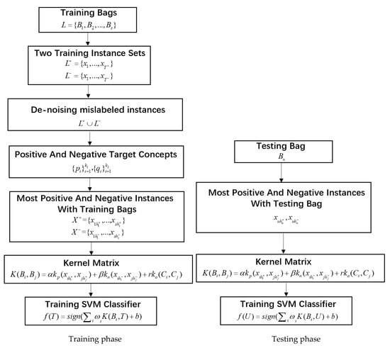
Figure 1.
Block diagram for the proposed algorithm.
4. MILDMS Algorithm
We introduce the MILDMS algorithm in this section, including four steps, i.e., target concept locating, instance de-noising, multiple part kernel construction, and MIL kernel construction. Before elaborating this algorithm, we first give a brief review of DD algorithm here, which works as constraint in our target concept obtaining process. The DD algorithm optimizes a DD function modeled on all training instances to directly locate the most diverse density point, while our MILDMS algorithm first finds the potential target concepts through optimizing and then verifying it by the DD constraints.
4.1. Review of Diverse Density (DD) Algorithm
As the most successful positive instance identification MIL algorithm, the DD method proposed by Maron attempts to locate the most diverse density point and then use it to infer instances’ labels [6]. Therefore, the bag label is determined by the most positive instance within bag. Assuming that there exists one single target which is denoted as , the diversity density function is defined as the probability on positive and negative bags.
The point, which maximizes the above function, is chosen as target concept. By assuming the conditional independence in all bags, a uniform prior over target concept and applying Bayes’ rules, we can rewrite Equation (4) as
To compute the in above formula, for the positive bag, Maron adopts the noisy-or model and define it as likewise, . Here, the probability of an instance to a potential target can be defined as . The optimization problem can be solved by gradient descent approach with multiple starting points to locate the target concept .
4.2. Target Concept Locating
Due to the successes of DD algorithm, we decided to adopt the DD constraint to our target concept locating model by especially considering how to overcome the shortcoming of the DD algorithm. To obtain meaningful results, we begin with analyzing the limitation of the DD function. Equation (5) contains two parts, and . These two parts work together to make the obtained target concept close to positive instances and far away from the negative instances. Unfortunately, the mislabeled training bags will greatly influence the DD function value, leading to a wrong target concept, as the target concept is modeled on the whole positive and negative bag space. To overcome this problem, we advocate here to model the target concept locating model in positive and negative bag space separately with the DD constraint. To avoid the noise data’s influence on DD function, we choose P nearest instances to these target concepts to calculate the DD function, where P equals the positive or negative bag number.
To facilitate the expressing, we first give some symbol notation. Suppose in MIL there are potential positive target concepts and potential negative target concepts negative target concepts, we use auxiliary variables to indicate the instance belongs to the potential positive target concept . That is to say, each can take values in , and implies the instance belongs to potential positive concept target . Taking the similar way, we define to represent whether the instance belongs to potential negative target concept . Here, is used to denote the P-nearest instances of point , and denote integer number. and are the instance numbers of all positive and negative bags separately. With these ingredients, we now define the target concept locating optimization problem as follow
where is the diversity density (DD) function, is the 2-norm of vector.
In a matrix form, Equation (6) can be written as
where and are the two sets generated by all the instances in positive training bags or negative training bags separately, and are the potential positive and negative target concepts, and is the Frobenius norm of matrix. In Equation (7), and are the two indicator matrixes whose entry can be 0 or 1, and when the -th entry of column is equal to 1, it means the instance belongs to the potential target concept .
To analyze the optimization (Equation (7)) more clearly, we split the constraints into four parts and name them C1, C2, C3, and C4, and convert it to formulate Equation (8)
Obviously, C1 requires each instance of or to only belong to one potential target concept; C2 means we can choose any integer number as target concept number; C3 chooses the most positive and negative target concepts from the potential target concept and which contain more instances than others; C4 encodes the DD constraint to our model which ensures the most positive target concept obtains the maximum DD value of its nearest p neighbor instances, while the most negative target concept obtains the minimum DD value.
For the , in above optimization problem (Equation (7)) is discrete variables and , belong to , it is both a combinatorial and integer optimization problem, which is NP-hard. To make this optimization problem solvable, we split it to two more easier problems. One of them is a much simpler optimization problem and another is constraint.
We split the optimization (Equation (8)) to below two parts (named as OP1 and CS1), where the first one is the objective function with constraint C1, C2 and the other is constraints C3 and C4.
Unfortunately, the OP1 of Equation (9) is still an integer programming and combinatorial optimization problem that cannot be solved easily. It is trivial to ignore CS1 constraint variables and . Then we can have two separate sub-problems from OP1.
Each is a clustering problem, which can find a local minimum by iterative, alternating optimization with respect to and , , and .
After obtaining the potential positive and negative target concepts and , we choose the most positive and negative target concepts and by using constraint C3, which means the column of matrix and that contain more non-zero entries than others will be selected as most positive and negative target concepts. Then, the next step is to determine whether and satisfy the constraint C4. For each potential target concepts in and , we choose the nearest neighbor instances, where the can be any integer number. Thus we can obtain instance set and around the potential positive and negative target concepts and . Since our DD function is based on instances not bags, our function can be rewritten as
where , . If the formula C4 is satisfied, the most positive and negative target concepts of MIL are obtained.
4.3. De-Noising Mislabeled Instances
Since the noise data will greatly influence MIL performance, we also perform a special process to de-noise the noise instances, which is based on a trivial idea that the positive instances should be in the most positive target concept region and far away from the most negative target concept region. In short, the positive instances should be closer to positive concepts and negative instances closer to negative concepts. For two class classification problem, we can treat one class as positive, another class as negative. Therefore, we define a function in Equation (12) to choose the mislabeled noise instance , which will be deleted from training sets ,
where is the 2-norm of vector, is used to represent the label of a bag. Here we need to remember that Equation (12) can not only de-noise the mislabeled instances but also delete the negative instances in positive bags, which will be helpful for alleviating the ambiguous problem existing in MIL.
4.4. Multiple Part Similarity Kernel Construction
Once the most positive and negative target concepts and are selected, we can easily choose the most positive and negative instance for each bag. We choose the instances nearest to these two target concepts as the most positive and negative instances in the bag. The index of most positive and negative instances choosing formula can be formula as below
where is an instance in bag , is the 2-norm of vector. Therefore we can obtain one most positive and one most negative instance denoted as and in bag .
As discussed in Section 3, the label of bag largely depends on the similarity between the instances , in bag computed by a traditional kernel, such as radical basis function (RBF). The other instances excluding the most positive and negative instances in different bags, denoted as , , is still a special set similarity problem named multiple part similarity.
As reported in [31], the Earth Mover’s Distance (EMD) can help to deal with the multiple part similarity problem, such as SIFT matching problem, histogram-based local descriptor comparing, etc. Thus, one possible way to compute the similarity between set and is to use a kernel function based on EMD distance.
To embed our multiple part similarity problem to EMD framework, we firstly line up all the instances in set and generate a new set . Here, we further represent the suppliers of EMD as , where , is the cardinal of , and the is the weight of the supplier . Normally, the weight is used as the total supply of suppliers or the total capacity of consumers in the EMD. Since all the instances in the set play equal role in set similarity, we set ’s value as . Similarly, we also denote the set as , where and . Letting represent the distance between supplier and consumer and defined as , the EMD optimization problem between set and can be defined as
Finally, the EMD distance between set and can be computed as
where is the optimal flow that can be determined by solving above Equation (14) with the standard simplex method. Note the can also be interpreted as the optimal match between the instance and in bag and , and meanwhile the EMD distance between two sets and is non-negative and symmetrical, thus we incorporate EMD distance into the Gaussian function to construct the multiple part similarity kernel
4.5. MIL Kernel Construction
To construct the MIL kernel, we need to model these similarities, including the most positive instance, most negative instance, and multiple part similarities, in a unified framework. Note the multiple kernel learning [32] has shown considerable success in computing multiple information similarities, here we incorporate these similarities to multiple kernel framework.
The key idea of multiple kernel is to construct a new kernel by linearly combining some pre-defined kernels. The multiple kernel is actually a convex combination of pre-defined kernel
where is the total number of kernels, and is any kernel function meeting the mercer condition.
Therefore, the objective of multiple kernel for MIL is to learn both the coefficients and the weights in the below quadratic optimization problem
where and are two bags in MIL, is the total number of kernels, and denote the -th base kernel and its weights respectively, is the penalty parameter to control the trade-off between accuracy and regularization. The MIL classifier is defined as
where and are obtained optimal decision variables from Equation (19) and the can be computed by the below formula
By integrating the multiple part similarity kernel defined in Equation (16) with most positive instance kernel and most negative instance kernel, our MIL kernel can be defined as
where and are the most positive instances, and are the most negative instances in bag Bi and Bj, Ci and Cj are two sets that satisfy and , and are the kernel functions used to compute the most positive and negative instance similarity, and is the predefined multiple part similarity kernel.
Based on the aforementioned fact that MIL contains two cases—one target concept and multiple target concepts problem—we can see that in the case of one target concept the most positive and negative instances in the bag can determine the label of the bag without the multiple part similarity kernel, thus the MIL kernel can be reduced to
To distinguish between one target concept and multiple target concepts, we compute the total numbers of instances contained by and , and compute the ration between the two biggest numbers of them which are compared to a threshold θ given in advance. Indeed, the total number of instances contained in P and Q can be easily obtained by counting none-zero entries in each row of matrix δ and in Equation (11). Since the entries and are either 0 or 1, the numbers of instances contained in and can be computed as
where is 1-norm of vector, and . We sort the set and by descending order, and obtain the two biggest number from the sorted set and denoted as and , and . Then, the formula used to classify one target concept and multiple target concepts can be defined as
It is not difficult to see that the MIL will be a one target concept when equals 1, otherwise will be multiple target concepts. In this paper, the is chosen to be 0.1.
4.6. Feature Extraction
Feature extraction plays the core role in image understanding either the one target concept or multiple target concepts in MIL. Thus, it is very important to choose suitable features to represent the image.
Now there are two ways to extract the image feature: hand-crafted and deep learning methods; while the hand-crafted methods benefit from professional human knowledge, which is in certain domains very important (see e.g., [33]), the deep learning methods benefit from large amounts of data sets (big data) and from deep network structures. To compare fairly with existing methods which adopt the hand-crafted features in MIL, we took the similar way to acquire the nine-dimension feature vector, including the color, texture, and shape of the five regions in the image, whose details can be found in [11].
In view of the powerful representation ability of convolutional neural networks (CNN), we used CNN to extract deep features. For the performance of reusing the existing deep learning architecture and find-tuning pre-trained model, we adopt below the network architecture and training strategy.
(1) Architecture: As an efficient CNN framework, VGG-16 contains in total 16 weight layers, 13 layers of which are convolutional layers and the other three of which are fully connected layers. The second fully connected layers are 4096 units whose output are used as features. To make the VGG-16 fit our MIL task, we replaced the last 1000-way fully connected layer with a two-way fully connected layer and used softmax function as the final prediction function.
(2) Network Training: The network was first pretrained on ImageNet dataset and then fine-tuned. We used stochastic gradient descent to fine-tune our network with a batch size of 128, learning rate of 0.0001, momentum of 0.9, and weight decay of 0.0005. We stopped our training after 36 epochs since the accuracy stops increasing.
4.7. Algorithm View
We summarize our MILDMS below. To facilitate expression, we denote the training bag set as two set union , p positive and q negative bags, and denote the instances from all the positive bags as , instances from negative bags as . Algorithm 1 was used to learn a MIL classifier defined by , and the input was maximum target concept number M.
| Algorithm 1. Learning MIL Classifier |
| Repeat iterations Fork+ = 1: M For k− = 1: M
End Until the constraint C4 is met For (each training bag Bi in set B)
Optimize Equation (18) to obtain the decision variables |
The code for unknown bag classification is in Algorithm 2 given below. The input is an unknown bag set , which is classified as positive by a bag classifier .
| Algorithm 2. Classifying MIL Bag |
For (each unknown bag Bi in set U)
|
5. Experiments
To evaluate the performance of our MILDMS, in this section, we conduct experiments on both two MIL datasets, the standard MIL dataset and image classification dataset. Here we use the standard MIL dataset to show the effectiveness of the MILDMS to deal with the one target concept in MIL and compare it with APR [5], SMILE [20], MILES [12], Attention and Gated-Attention [25], DD [6], DD-SVM [11], and MI-Net with DS [24]. For the object detection and image classification task, we applied the above Section 4.6 to extract the image features. Additionally, the Elephant, Fox, Tiger and PASCAL VOC 2007 and 2012 were used to show the performance on one target concept MIL and the COREL dataset shows the generality of our MIL method in multiple concepts detection.
For all our experiments, we fixed the maximum number of target concepts to 10. Gaussian function was chosen as the positive and negative instance similarity kernels and the regularization parameter C of Equation (18) was chosen by 5-fold cross validation on the training data using grid search. The threshold in Equation (24) was used to classify the one target and multiple target concepts problem was fixed to 0.1 which was determined by many trials by letting range from 0.1 to 0.9.
We applied the SimpleMKL [32] software toolkit to solve the multiple kernel learning. The clustering problem existing in Equation (10) was solved by Cartesian k-means [34].
5.1. Standard MIL Dataset
We first chose the most commonly used MIL dataset, MUSK dataset, to test our algorithm MILDMS. As a drug activity task, the MUSK dataset contains MUSK1 and MUSK2, where the former contains 47 positive bags and 45 negative bags with the bag instance number in the range from 2 to 40, while the latter contains 39 positive bags and 63 negative bags with the bag instance number in the range from 1 to 1044. Table 1 summarizes data sets according to the number of positive and negative bags, instances and features. Additionally, we also used a well-known three image class problem to verify the efficiency of our MILDMS, which has three classes Elephant, Fox, and Tiger, and each image is segmented into regions, with features given by color, texture, and shape [11].

Table 1.
Multiple instance learning (MIL) data sets, with the respective number of positive and negative bags, features, and instances.
We report our experimental result in Table 2, which indicates that our MILDMS is highly competitive with other state-of-the-art MIL methods. In Table 2, our MILDMS achieves the best result on MUSK2, Elephant, Tiger, Fox, and is competitive with SMILE [20], and also achieves higher classification precision than deep learning methods MI-Net with DS [24], Gated-Attention, and Attention [25].
Table 2.
Results (in %) of proposed MILDMS, and many of the MIL algorithms available in the literature, with results provided for both MUSK and Images data sets.
5.2. Object Detection
In order to further test the performance of MILDMS on one target concept MIL, we evaluated our method on the challenging PASCAL VOC 2007 and 2012 [35] which have 9962 and 22,531 images respectively. In these two datasets, the total 9962 and 22,531 images were divided into 20 distinct categories, which are person, bird, cat, cow, dog, horse, sheep, airplane, bicycle, boat, bus, car, motorbike, train, bottle, chair, dining table, potted plant, sofa, and tv/monitor.
For the object detection task, we compared our method with SMILE [20], MILES [12], Gated-Attention [25] and MI-Net with DS [24] algorithms, and report their average accuracy of 20 classes shown in Figure 2. As can be seen from Figure 2, our MILDMS achieves the best results and far exceeds the other MIL algorithms including traditional methods and deep learning methods in the object detection task. The reason lies in that positive and negative instances of images are generated by hand-crafted and deep features with DD constraint, which can fully utilize the features.
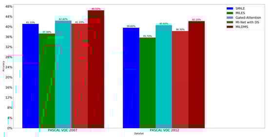
Figure 2.
The comparison between our method and other methods on PASCAL VOC 2007 and 2012.
5.3. Image Classification Application
In addition, we also applied our MILDMS to an image classification task dataset COREL, which contains 20 categories, including Africa people and villages, Beaches, Historical buildings, Buses, Dinosaurs, Elephants, Flowers, Horses, Mountains and glaciers, Food, Dogs, Lizards, Fashion models, Sunset scenes, Cars, Waterfalls, Antique furniture, Battle ships, Skiing, and Desserts. In the dataset, the total 2000 images were divided into 20 distinct categories, where each category contains 100 images. We selected one sample image from each of the 20 categories and display them in Figure 3. The categories are ordered in a row-wise manner from the upper-leftmost image (Africa people and villages) to the lower-rightmost image (Desserts).

Figure 3.
Sample images from the 20 categories of the COREL image set.
We report our MILDMS on COREL dataset in Table 3. The result show that the proposed method also yields competitive results for the COREL 2000 image set. Compared with other MIL methods, such as SMILE [20], MILES [12], DD-SVM [11], Attention and Gated-Attention [25], and MI-Net with DS [24], our algorithm achieves the best performance. The reason is that our method can capture the multiple concepts of images and combine them together to achieve good performance.
Table 3.
Results (in %) for COREL 2000: average accuracy, and the 95%-confidence interval (in brackets).
5.4. Sensitivity to Labeling Noise
Labeling noise is an unavoidable problem in the real image application because labeling data requires long and difficult work, and it is easy to make mistakes. Thus, we designed a labeling noise condition to verify our algorithms’ performance. To be fair, we also adopted the same noise sensitivity setting that was evaluated by the MILES [12] on COREL dataset. We compared MILDMS with MILES [12], SMILE [20], DD-SVM [11], Attention and Gated-Attention [25], MI-Net with DS [24] on Category 3 (Historical building) and Category 8 (Horses) of the Corel 2000 image set, on which we added d% of noise by changing the labels of d% of positive bags and d% of negative bags. Under different noise levels, we randomly split the image set into two same size sub-sets as training and test sets 20 times and report the average classification accuracy in Figure 4.
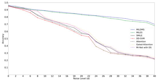
Figure 4.
Sensitivity to labeling noise.
As shown in Figure 4, our MILDMS is more robust than DD-SVM and SMILE in high noise level, for our method is modeled in positive and negative instance space separately. It is worth noticing that our MILDMS algorithm achieves equal performance when comparing with MILES, and outperforms deep MIL methods including Attention and Gated-Attention [25], and MI-Net with DS [24].
6. Conclusions
Multiple instance learning constitutes a framework for classification problems with ambiguity problems in instance labelling. In this paper, we introduced a new approach called MILDMS in which most positive and negative instances, generated by hand-crafted and deep features, are based on DD constraint. In addition, we integrated the multiple part similarity into our framework, which yields the capacity of performing well in MIL datasets. The experiments demonstrate the usage of the method MILDMS which is comparable to the state-of-the-art MIL algorithms. There are more interesting directions to investigate in the future. First, we could find a more efficient and effective way to deal with our optimization problem. Second, we would like to find the explainability of our method using explainable artificial intelligence (AI) methods.
Author Contributions
Conceptualization, methodology and writing, C.W.; review and editing, Z.L. and J.Q.; data curation, Q.F. and A.L.
Funding
This research was funded by China Postdoctoral Science Foundation, grant 2014M552479 and grant 2014M552478, Humanities and Social Science Funded Project of Ministry of Education of China, grant 17YJCZH186, Natural Science Basic Research Plan in Shaanxi Province of China, grant 2013JQ8022, and Scientific Research Project of Education Department of Shaanxi Province of China, grant 2013JK1181 and grant 2014JK1724.
Conflicts of Interest
The authors declare no conflict of interest.
References
- Liu, B.; Xiao, Y.; Hao, Z. A Selective Multiple Instance Transfer Learning Method for Text Categorization Problems. Knowl. Based Syst. 2018, 141, 178–187. [Google Scholar] [CrossRef]
- Hu, K.; He, W.; Ye, J.; Zhao, L.; Peng, H.; Pi, J. Online Visual Tracking of Weighted Multiple Instance Learning via Neutrosophic Similarity-Based Objectness Estimation. Symmetry 2019, 11, 832. [Google Scholar] [CrossRef]
- Yuan, C.H.; Xu, C.Y.; Wang, T.J.; Liu, F.; Zhao, Z.; Feng, P.; Guo, J. Deep multi-instance learning for end-to-end person re-identification. Multimed. Tools Appl. 2018, 77, 12437–12467. [Google Scholar] [CrossRef]
- Manivannan, S.; Cobb, C.; Burgess, S.; Trucco, E. Subcategory Classifiers for Multiple-Instance Learning and Its Application to Retinal Nerve Fiber Layer Visibility Classification. IEEE Trans. Med. Imaging 2017, 36, 1140–1150. [Google Scholar] [CrossRef] [PubMed]
- Dietterich, T.G.; Lathrop, R.H.; Lozano-Perez, T. Solving the multiple instance problem with axis-parallel retangles. Artif. Intell. 1997, 89, 31–71. [Google Scholar] [CrossRef]
- Maron, O. Learning from Ambiguity. Ph.D. Thesis, MIT, Cambridge, MA, USA, 1998. [Google Scholar]
- Wang, J.; Zucker, J.D. Solving the multiple instance problem: A lazy learning approach. In Proceedings of the International Conference on Machine Learning (ICML), Stanford, CA, USA, 28 June–1 July 2001; pp. 1119–1126. [Google Scholar]
- Zhang, Q.; Goldman, S.A. Em-dd: An improved multiple-instance learning. In Proceedings of the Advances in Neural Information Processing Systems (NIPS), Vancouver, BC, Canada, 3–8 December 2001; pp. 1073–1080. [Google Scholar]
- Gartner, T.; Flach, P.A.; Kowalczyk, A.; Smola, A.J. Multi-instance kernels. In Proceedings of the International Conference on Machine Learning (ICML), Sydney, Australia, 8–12 July 2002; pp. 179–186. [Google Scholar]
- Andrews, S.; Tsochantaridis, I.; Hofmann, T. Support vector machines for multiple-instance learning. In Proceedings of the Advances in Neural Information Processing Systems (NIPS), Vancouver and Whistler, British Columbia, BC, Canada, 8–13 December 2003; pp. 561–568. [Google Scholar]
- Chen, Y.; Wang, J.Z. Image categorization by learning and reasoning with regions. J. Mach. Learn. Res. 2004, 5, 913–939. [Google Scholar]
- Chen, Y.; Bi, J.; Wang, J. Miles: Multiple-instance learning via embedded instance selection. IEEE Trans. Pattern Anal. Mach. Intell. 2006, 28, 1931–1947. [Google Scholar] [CrossRef]
- Zhou, Z.H.; Xu, J.M. On the relation between multi-instance learning and semi supervised learning. In Proceedings of the International Conference on Machine Learning (ICML), Corvallis, OR, USA, 20–24 June 2007; pp. 1167–1174. [Google Scholar]
- Zhou, Z.H.; Sun, Y.Y.; Li, Y.F. Multi-instance learning by treating instances as non-i.i.d. samples. In Proceedings of the International Conference on Machine Learning (ICML), Montreal, QC, Canada, 14–18 June 2009; pp. 1249–1256. [Google Scholar]
- Fu, Z.; Robles-Kelly, A.; Zhou, J. MILIS: Multiple instance learning with instance selection. IEEE Trans. Pattern Anal. Mach. Intell. 2011, 33, 958–977. [Google Scholar]
- Erdem, A.; Erdem, E. Multiple-instance learning with instance selection via dominant sets. Lect. Notes Comput. Sci. SIMBAD 2011, 7005, 177–191. [Google Scholar]
- Zhang, D.; He, J.R.; Si, L.; Lawrence, R. MILEAGE: Multiple Instance Learning with Global Embedding. In Proceedings of the International Conference on Machine Learning (ICML), Atlanta, GA, USA, 16–21 June 2013; pp. 82–90. [Google Scholar]
- Nguyen, D.T.; Nguyen, C.D.; Hargraves, R.; Kurgan, L.A.; Cios, K.J. mi-DS: Multiple-Instance Learning Algorithm. IEEE Trans. Cybern. 2013, 43, 143–154. [Google Scholar] [CrossRef]
- Li, Z.; Geng, G.H.; Feng, J.; Peng, J.Y.; Wen, C.; Liang, J.L. Multiple instance learning based on positive instance selection and bag structure construction. Pattern Recogn. Lett. 2014, 40, 19–26. [Google Scholar] [CrossRef]
- Xiao, Y.; Liu, B.; Hao, Z.; Cao, L. Smile: A similarity-based approach for multiple instance learning. IEEE Trans. Cybern. 2014, 44, 500–515. [Google Scholar] [CrossRef] [PubMed]
- Zhang, Y.L.; Zhou, Z.H. Multi-instance learning with key instance shift. In Proceedings of the International Joint Conference on Artificial Intelligence (IJCAI), Melbourne, Australia, 19–25 August 2017; pp. 3441–3447. [Google Scholar]
- Küçükaşcı, E.S.; Baydoğan, M.G. Bag encoding strategies in multiple instance learning problems. Inform. Sci. 2018, 32, 654–669. [Google Scholar] [CrossRef]
- Wu, J.; Pan, S.; Zhu, X.; Zhang, C.; Wu, X. Multi-instance learning with discriminative bag mapping. IEEE Trans. Knowl. Data Eng. 2018, 30, 1065–1080. [Google Scholar] [CrossRef]
- Wang, X.; Yan, Y.; Tang, P.; Bai, X.; Liu, W. Revisiting Multiple Instance Neural Networks. Pattern Recogn 2016, 74, 15–24. [Google Scholar] [CrossRef]
- Maximilian, I.; Jakub, M.T.; Max, W. Attention-based Deep Multiple Instance Learning. In Proceedings of the International Conference on Machine Learning (ICML), Stockholm, Sweden, 10–15 July 2018; pp. 2127–2136. [Google Scholar]
- Liu, X.; Jiao, L.; Zhao, J.; Zhao, J.; Zhang, D.; Liu, F.; Yang, S.; Tang, X. Deep Multiple Instance Learning-Based Spatial–Spectral Classification for PAN and MS Imagery. IEEE Trans. Geosci. Remote. Sens. 2018, 56, 461–473. [Google Scholar] [CrossRef]
- Li, X.; Zhang, Y.; Cui, Q.; Yi, X.; Zhang, Y. Tooth-Marked Tongue Recognition Using Multiple Instance Learning and CNN Features. IEEE Trans. Cybern. 2019, 49, 380–387. [Google Scholar] [CrossRef]
- Wu, J.J.; Yu, Y.N.; Huang, C.; Yu, K. Deep multiple instance learning for image classification and auto-annotation. In Proceedings of the IEEE Conference on Computer Vision and Pattern Recognition (CVPR), Boston, MA, USA, 7–12 June 2015; pp. 3460–3469. [Google Scholar]
- Lowe, G.D. Distinctive Image Features from Scale-Invariant Interest Points. Int. J. Comput. Vis. 2004, 60, 91–110. [Google Scholar] [CrossRef]
- Grauman, K.; Darrell, T. The pyramid match kernel: Efficient learning with sets of features. J. Mach. Learn. Res. 2007, 8, 725–760. [Google Scholar]
- Rubner, Y.; Tomasi, C.; Guibas, L. The Earth Mover’s Distance as a Metric for Image Retrieval. Int. J. Comput. Vis. 2000, 40, 99–121. [Google Scholar] [CrossRef]
- Rakotomamonjy, A.; Bach, Y.; Grandvalet, Y. SimpleMKL. J. Mach. Learn. Res. 2008, 9, 2491–2521. [Google Scholar]
- Holzinger, A.; Plass, M.; Kickmeier-Rust, M.; Holzinger, K.; Crişan, G.C.; Pintea, C.-M.; Palade, V. Interactive machine learning: Experimental evidence for the human in the algorithmic loop. Appl. Intell. 2019, 49, 2401–2414. [Google Scholar] [CrossRef]
- Norouzi, M.; Fleet, D. Cartesian k-means. In Proceedings of the IEEE Conference on Computer Vision and Pattern Recognition (CVPR), Portland, OR, USA, 23–28 June 2013; pp. 3017–3024. [Google Scholar]
- Everingham, M.; Van Gool, L.; Williams, C.K.; Winn, J.; Zisserman, A. The pascal visual object classes (VOC) challenge. Int. J. Comput. Vis. 2010, 88, 303–338. [Google Scholar] [CrossRef]


© 2019 by the authors. Licensee MDPI, Basel, Switzerland. This article is an open access article distributed under the terms and conditions of the Creative Commons Attribution (CC BY) license (http://creativecommons.org/licenses/by/4.0/).