A Novel Identification Method for Apple (Malus domestica Borkh.) Cultivars Based on a Deep Convolutional Neural Network with Leaf Image Input

Abstract

The innovation of germplasm resources and the continuous breeding of new varieties of apples (Malus domestica Borkh.) have yielded more than 8000 apple cultivars. The ability to identify apple cultivars with ease and accuracy can solve problems in apple breeding related to property rights protection to promote the healthy development of the global apple industry. However, the existing methods are inconsistent and time-consuming. This paper proposes an efficient and convenient method for the classification of apple cultivars using a deep convolutional neural network with leaf image input, which is the delicate symmetry of a human brain learning. The model was constructed using the TensorFlow framework and trained on a dataset of 12,435 leaf images for the identification of 14 apple cultivars. The proposed method achieved an overall accuracy of 0.9711 and could successfully avoid the over-fitting problem. Tests on an unknown independent testing set resulted in a mean accuracy, mean error, and variance of ${\mu }_{acc}=0.9685$, ${\mu }_{\epsilon }=0.0315$, and ${\sigma }^2=1.89025E-4$, respectively, indicating that the generalization accuracy and stability of the model were very good. Finally, the classification performance for each cultivar was tested. The results show that model had an accuracy of 1.0000 for Ace, Hongrouyouxi, Jazz, and Honey Crisp cultivars, and only one leaf was incorrectly identified for 2001, Ada Red, Jonagold, and Gold Spur cultivars, with accuracies of 0.9787, 0.9800, 0.9773, and 0.9737, respectively. Jingning1 and Pinova cultivars were classified with the lowest accuracies, with 0.8780 and 0.8864, respectively. The results also show that the genetic relationship between cultivars Shoufu 3 and Yanfu 3 is very high, which is mainly because they were both selected from a red mutation of Fuji and bred in Yantai City, Shandong Province, China. Generally, this study indicates that the proposed deep learning model is a novel and improved solution for apple cultivar identification, with high generalization accuracy, stable convergence, and high specificity.

1. Introduction

The apple (Malus domestica Borkh.) originated in Europe, Asia, and North America [1,2,3]. As a result of the strong adaptability and high tolerance of this species to different soil and climatic conditions, and aligning with natural domestication and artificial breeding improvements, apple cultivars are now grown on five continents [2,3]. To date, more than 8000 apple cultivars have been bred to cater to specific demands, which vary greatly across the globe [4]. In 2018, the global production of apples—the second most popular fruit—was over 68.6 million tons, despite the frost disaster in China and Iran that reduced it to the lowest level in eight years [5]. Furthermore, the global apple demand is increasing at a robust pace, driven mainly by the increase in its daily consumption as a fresh fruit and its use in medicine and the cosmetic industry as an essential ingredient. As it is affordable and has longstanding associations with healthy lifestyles, its processed products such as juice, vinegar, cider, and jam are in extremely high demand throughout the year, especially in America, Europe, Russia, and Egypt [6].

Apple germplasm resources are rich and widely distributed throughout the world, with a long history of commercial cultivation. With the innovation of germplasm resources and the continuous selection of new apple varieties, apple cultivars are frequently mixed, and the phenomenon of homonymy is more serious than ever before. Currently, the ability to identify apple cultivars efficiently, easily, and accurately is a continuous hot topic that has attracted the attention of breeding experts and horticultural experts worldwide.

Traditionally, to classify a cultivar, gardeners or breeders have primarily relied on their own intuition and expertise in on-site observation and analysis of the botanical characteristics of the fruit, tree, branch, and leaf in orchards. However, concerns regarding this method include its lack of objectivity, low efficiency, and unpredictable accuracy; furthermore, it is unquantifiable and unsuitable for large-scale orchard work because it highly depends on personal empirical knowledge and cognition. The other method relies on experts to systematically test the fruit’s physiological indicators in a laboratory using a combination of physical, chemical, molecular, and biological technologies. However, this approach is not only expensive and time-consuming, but also involves complicated operating procedures and is incredibly unfriendly to common growers [7,8,9].

With the application of digital image processing technology and computer vision technology in agriculture, many machine learning methods for plant classification using leaf images have been proposed and studied such as the k-nearest neighbors (KNN), decision tree, support vector machine (SVM), and naive Bayes (NB) [10,11,12,13,14,15]. However, a common and serious disadvantage is the need to manually design and extract discriminative features before the classification of different plants. Moreover, the features designed and extracted for a specific plant are not suitable for other plants, so they must be redefined when the same method is applied to new cases. The processes of designing and extracting features are difficult and strategic. Furthermore, although these methods have shown good results with improved accuracy, they are susceptible to artificial feature selection and are not robust or stable enough to meet the needs of actual scientific research and production. In recent years, the convolutional neural network (CNN) has been developed as one of the best classification methods for computer pattern recognition tasks [16,17,18,19,20,21,22,23,24,25,26,27,28,29,30,31] because discriminative features can be automatically extracted and fused from a low layer to a high layer through multiple layers of convolutional operations. The breakthrough application of the convolutional neural network in image-based recognition has inspired its wide use in studies on plant classification and recognition in precision agriculture.

2. Related Works

Related research works include Mads Dyrmanna et al. [16], who designed a convolutional neural network to classify 22 weed and crop species at early growth stages and achieved a total classification accuracy of 86.2%. Hulya Yalcin et al. [17] proposed a convolutional neural network structure to classify different crops using leaf images. They tested the performance of the method on the TARBIL project dataset supported by the Turkish government, and the results confirmed its effectiveness. Lee, Sue Han et al. [18] proposed a hybrid general organ convolutional neural network (HGO-CNN) that performs classification using different numbers of plant views by optimizing the context-dependence between views, and verified the performance of this method on the benchmark dataset plantclef2015 [19]. Although these studies aimed to classify different plant species, they were based on the common fact that their leaves have different colors and shapes, which makes the classification task easier. In contrast, the leaves of apple cultivars are generally the same color and similar in shape, so using these methods to classify apple cultivars with leaf images is exceedingly challenging and problematic. Sue H. L. et al. [20] proposed a method to extract leaf features using a CNN and reported that different orders of venation are more representative features than shape and color. Guillermo L. G. [21] proposed the use of a deep convolutional neural network (DCNN) to classify three different legume species. Baldi A. [22] proposed a leaf-based back propagation neural network for the identification of oleander cultivars. Although these three studies did not involve the classification of apple cultivars, their achievements are important references for this study.

In summary, plant classification using a convolutional neural network with leaf image input has become both a focus and challenge in precision agriculture, which has attracted extensive attention from scholars worldwide, but is still in its infancy with few related research achievements, especially on apple cultivar classification. Therefore, in this paper, we present a novel identification approach for apple cultivars based on the deep convolutional neural network—a DCNN-based model—with apple leaf image input.

The DCNN-based model must solve two tricky problems. First, insufficient apple leaf images taken in natural environments can be a major obstacle in training the model to produce a high generalization performance. Second, determining the best structure of the model is a technological barrier to success.

The main contributions of this paper can be summarized as follows:

• Sufficient apple leaf samples were obtained as research objects by choosing 14 apple cultivars, most of which grow in Jingning County, Gansu Province, which is the second-largest apple production area in the Loess Plateau of Northwest China. We took apple leaf images in the orchard under natural sunlight conditions at a resolution of 3264 × 2448 and/or 1600 × 1200 from multiple angles in automatic shooting mode to capture diverse apple leaf images to train the DCNN-based model. In particular, the diversity of leaf images increased under various weather conditions by capturing leaf images for 37 days from 15 July 2019 to 20 August 2019. This period included sunny, cloudy, rainy (light rain, moderate rain, rain, heavy rain), and foggy days. Finally, a total of 12,435 leaf images from 14 apple cultivars were obtained. This large number and wide range can enhance the robustness of the DCNN-based model in the training process and ensure that it has a high generalization capability.
• A novel deep convolutional neural network model with leaf image input was proposed for the identification of apple cultivars through the analysis of the characteristics of apple cultivar leaves. The convolution kernel size and number were adjusted, and a max-pooling operation after each convolution layer was implemented; dropout was used after the dense layer to prevent the over-fitting problem.

The remainder of this paper is organized as follows. In Section 3, the apple cultivars, the method of acquiring apple leaf images, and the software and computing environment are introduced. In Section 4, the construction of the novel deep convolutional neural network model is described. Section 5 analyzes the experimental results in detail. Finally, this paper is concluded in Section 6.

3. Acquisition of Sufficient Apple Cultivar Leaf Images

3.1. Plant Materials and Method

This study was conducted in the orchard of the Research Institute of Pomology of Jingning County (35°28′ N, 104°44′ E; elevation: 1600 m above sea level), located in Jingning County, Gansu Province, NW China. The 14 apple cultivars that were chosen as research objects in this study (Table 1) mainly grow in Jingning County, Gansu Province, which is the second-largest apple production area in the Loess Plateau of Northwest China. The main rootstocks are M series and SH series dwarfing rootstocks. More than 100 mature healthy leaves without mechanical damage, disease lesions, or insect pests were randomly picked from the branches at the periphery (more than 1.0 m from the trunk) and the inner bore (less than 0.5 m from the trunk) in four directions (east, west, south, and north) of the tree crown. A total of 2711 leaves were picked. Details about each cultivar are shown in Table 1. All trees were exposed to uniform farming practices and measures, edaphic and health conditions, and light intensity conditions. In particular, to increase the generalization performance of the DCNN-based model proposed in this paper, we deliberately magnified the classification challenge by selecting leaves with as many morphological differences as possible for each cultivar.

Table 1. The 14 apple cultivars used in this study.

Class ID	Abbreviation	Apple Cultivar	Leaves	Leaf Images
1	2001	2001	206	946
2	ACE	Ace	195	938
3	ADR	Ada Red	186	1029
4	FJMM	Fujimeiman	210	982
5	HANF	Hanfu	185	777
6	HRYX	Hongrouyouxi	196	779
7	JN1	Jingning 1	176	817
8	JAZ	Jazz	206	758
9	HOC	Honey Crisp	186	899
10	PIN	Pinova	207	879
11	JONG	Jonagold	184	887
12	SHF3	Shoufu 3	174	1017
13	GOS	Gold Spur	204	756
14	YANF3	Yanfu 3	196	971
Total			2711	12,435

3.2. Acquisition of Sufficient Apple Cultivar Leaf Images

An appropriate leaf image database plays a crucial role in this type of machine learning model [14]. Only leaf images that are taken in the natural environment can adequately test the generalization performance of the classification/identification model. Immediately after a leaf was picked from the tree, it was placed on the surface of a white piece of paper on the flat ground beside the fruit tree, and images were taken immediately under natural sunlight conditions at an image resolution of 3264 × 2448 and/or 1600 × 1200 from multiple angles in automatic shooting mode. The digital color camera used was a Nikon Coolpix B700 (60× optical zoom Nicol lens, 1/2.3-inch CMOS sensor), and the image type was RGB 24-bit true color. In particular, the diversity of leaf images was increased by obtaining images under various weather conditions: the test period in which the leaf images were captured was 37 days (from 15 July 2019 to 20 August 2019), during which there were 12 sunny days, 16 overcast days, one day of light rain, one day of moderate rain, one day of heavy rain, five cloudy days, and one foggy day (see www.weather.com.cn for details) [23]. On rainy days, the leaves had hardly been picked and photographed when the rain stopped. Finally, 12,435 diverse leaf images from 14 apple cultivars were obtained. The images were numbered with Arabic numerals starting from zero by cultivar Class ID. The Class IDs of each cultivar are shown in Table 1, along with the number of leaves and images for each cultivar. The size of the images was compressed to 512 × 512 to reduce the training time.

Examples of leaf images for all 14 cultivars are shown in Figure 1. The leaf images in this figure, from left to right, correspond to the cultivars with Class IDs 1–14, as specified in Table 1. Figure 1 reveals that apple leaves are generally very simple and similar to each other; they have an elliptical-to-ovate shape and dimensions of about 4.5–10 and 3–5.5 cm in length and width, respectively, with a sharp apex and round and blunt serrated edges. Due to these similarities, classifying apple cultivars using leaf images is exceedingly complicated.

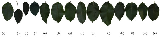
Figure 1. Example leaf images of 14 apple cultivars: (a–n) correspond to Class IDs 1–14 in Table 1.

3.3. Software and Computing Environment

The experiment was conducted on a Lenovo 30BYS33G00 computer with an Intel 3.60 GHz CPU, 16 GB memory, and parallel speedup by the NVIDIA GeForce1080 GPU. The NVIDIA GeForce1080 GPU has 2560 CUDA cores and 8 GB of HBM2 memory. The core frequency is up to 1607 MHz, and the floating-point performance is 10.6 TFLOPS. The DCNN-based model was implemented in the TensorFlow framework with the tensorflow.keras interface [27]. More detailed configuration parameters are presented in Table 2.

Table 2. Software and hardware environment.

Configuration Item	Value
Type and Specification	Lenovo 30BYS33G00
CPU	Intel® Xeon® W-2123 CPU @ 3.60 GHz (8 CPUs)
GPU	NVIDIA GeForce GTX 1080 8 GB
Memory	16 GB
Operating System	Windows 10 Professional (64-bit)
Integrated Development Environment	PyCharm Community 2019.2.3
Programming Language	Python 3.7
Experimental Results Analyzing Software	MATLAB R2010a

4. Generation of the Deep Convolutional Neural Network-Based (CNN-Based) Model for Apple Cultivar Classification

A deep convolutional neural network (DCNN) is a deep supervised machine learning model that is mainly composed of an input layer, convolution layer, pooling layer, activation function, full connection layer, and output layer. By simulating the learning mechanism of the human brain, DCNNs hierarchically process signals or data received in the input layer. After the input goes through multilayer perception and learning, it enters the full connection layer, where the comprehensive understanding acquired in the previous layers is fully connected to form the cognitive ability, which is used to classify and identify the target, as detailed in Figure 2.

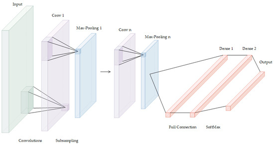
Figure 2. The deep convolutional neural network.

4.1. Construct the Deep Convolutional Neural Networks-Based (DCNNs-Based) Model for Apple Cultivar Identification with Leaf Image Input

Convolutional neural networks replace matrix multiplication with convolution, which is a special linear operation. Through multilayer convolution operations, the complicated features of images can be extracted from a low layer to a high layer. The front convolution layers capture local and detailed features in the image, while the rear layers capture more complex and abstract features; after several convolution layers, the abstract representation of the image at different scales is obtained.

There are many different convolution kernels in the same convolution layer; convolution kernels are equivalent to a group of bases and can be used to extract image features at different depths such as edges, lines, and angles. The weight parameters of a convolution kernel are shared by all convolution operations in the same layer, but the weight parameters of different convolution kernels are different from each other and serve as learnable parameters in DCNNs. In its local receptive field, each convolution kernel with the same weight parameters convolves with the neuron output matrix of the previous layer, and then a new neuron in this layer is created. By translating the local receptive field with a fixed step, the process is repeated, another new neuron is obtained, and this repetition continues until the neuron output matrix of this layer is obtained, which is the feature map (FM) corresponding to this convolution kernel. The FMs corresponding to all convolution kernels are combined to form the complete feature map output of this layer. The number of FMs is equal to the number of convolution kernels in this layer. The output of the previous layer is the input of the next layer, the input of the first convolution layer is the raw leaf image, and the output of the last layer is the input of the full connection layer. The output feature map can be described by Equation (1):

$$y_l^i=W_l{*x}_{l-1}^{n\times n}+b_l^{},$$

(1)

where $y_l^i$ is the ith neuron of the $l\mathrm{th}$ convolution layer, and $b_l^{}$ is the bias. $W_l$ represents the shared weight matrix of a convolution kernel of $n\times n$, and $x_{l-1}^{n\times n}$ represents the eigenvalues of the rectangular region of $n\times n$ in the input feature map.

The number of convolution operations can be reduced by using pooling technology with subsampling to reduce the size of the feature map obtained from the convolution layer. Generally, mean-pooling can mitigate the increase in accuracy variance caused by the limitation of the local receptive field, so more background information in the image is retained. On the other hand, max-pooling can reduce the deviation in the mean accuracy caused by errors in the convolution layer parameters, so more texture information is retained. In this study, we focused more on preserving the texture information of apple leaf images, so there was a max-pooling layer after each convolution layer. This approach can lead to faster convergence and improved generalization performance [24].

When the feature map $Y_l$ of the $l\mathrm{th}$ convolution layer is passed to the max-pooling layer, the max operation is applied to $Y_l$ to produce a pooled feature map $X_l$ as the output. As shown in Equation (2), the max operation selects the largest element:

$$X_l{}^j=\underset{i\in R_j}{\max }{Y}_l{}^i$$

(2)

where $R_j$ represents the $j\mathrm{th}$ pooling region in feature map $Y_l$; $i$ is the index of each element within $R_j$; and $X_l{}^j$ denotes the $j\mathrm{th}$ neuron of the $l$th pooled feature map [25].

The full connection layer, as the name implies, connects every neuron of the layer with all the neurons of the previous layer to combine the features extracted from the front and obtain the output, which is sent to the final classifier (such as the softmax classifier used in this study). That is, the full connection layer itself no longer has the ability to extract features, but attempts to use existing high-order features to complete the learning objectives.

In a convolutional neural network, the convolution operation is only a linear operation of weighted sums, so it is necessary to introduce nonlinear elements to the network to solve nonlinear problems. Therefore, an activation function, which is a nonlinear function, is included in the CNN. In this study, the ReLU activation function is used for the output of every convolution layer, and is shown in Equation (3):

$$\sigma (x)=\max (x,0)$$

(3)

When x < 0, its output is always 0. As its derivative is 1 when x > 0, it can maintain a continuously decreasing gradient, which can alleviate the problem of the disappearing gradient and accelerate the convergence speed.

In this study, the activation function used in the full connection layer was the softmax function, which is mainly used for multiclassification problems. Softmax maps the outputs of multiple neurons to the (0,1) interval, which can be regarded as the probability of belonging to a certain class. The softmax function is shown in Equation (4), where $v_i$ is the $i$th component element in a vector $v$.

$$softmax(v_i)=\frac{e^{v_i}}{{\displaystyle \sum _j\begin{array}{l}{e}^{v_j}\\ \end{array}}}$$

(4)

4.2. Specific Parameters of the DCNN-Based Model in This Study

This paper proposes a model based on a deep convolutional neural network to classify apple cultivars using leaf image input. The model architecture and related parameters are shown in Figure 3 and Table 3, respectively. The model consists of an input layer, six convolution layers, with each followed by a max-pooling layer, one standard one-dimensional dense full connection layer, one dropout process, and an output layer.

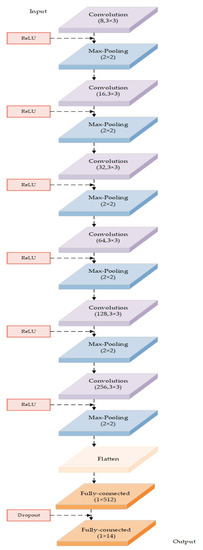
Figure 3. The architecture of the DCNN-based model in this study.

Table 3. Related parameters of the DCNN-based model.

Type	Patch Size/Stride	Output Size
Convolution	$3\times 3/2$	$8\times 512\times 512$
Pool/Max	$2\times 2/2$	$8\times 256\times 256$
Convolution	$3\times 3/2$	$16\times 256\times 256$
Pool/Max	$2\times 2/2$	$16\times 128\times 128$
Convolution	$3\times 3/2$	$32\times 128\times 128$
Pool/Max	$2\times 2/2$	$32\times 64\times 64$
Convolution	$3\times 3/2$	$64\times 64\times 64$
Pool/Max	$2\times 2/2$	$64\times 32\times 32$
Convolution	$3\times 3/2$	$128\times 32\times 32$
Pool/Max	$2\times 2/2$	$128\times 16\times 16$
Convolution	$3\times 3/2$	$256\times 16\times 16$
Pool/Max	$2\times 2/2$	$256\times 8\times 8$
Full Connection	-	512

In the TensorFlow framework with the tensorflow.keras interface, constructing the DCNN-based model for the classification of apple cultivars starts from the completion of its input layer by inputting the raw leaf images from 14 cultivars into the model, and ends with the fulfillment of its output layer by predicting the classification labels of leaf images.

The input format of the leaf image retains its original structure in a four-dimensional tensor as [number of images trained in a batch, image height, image width, number of image channels]. In this study, it was the float32 image of [32,512,512,3].

The output result is a classification probability list with a length of 14 (P1, P2, P3, P4, P5, P6, P7, P8, P9, P10, P11, P12, P13, P14), with each element in the list corresponding to the likelihood that the leaf belongs to each of the 14 apple cultivars in Table 1. The maximum value in the list, pmax = max (P1, P2, P3, P4, P5, P6, P7, P8, P9, P10, P11, P12, p13, P14), is the ultimate predicted classification label. In this study, if the predicted label is consistent with the actual label, then this leaf image sample is correctly classified/identified by the DCNN-based model.

The convolution layer of this model is represented by stage 1 in Figure 3. According to the features of the apple leaf images, we specifically designed all the convolution kernels’ sizes in each convolution layer as 3 * 3, stride = 1, pad = 1, which can gradually extract the features of the leaf image and ensure that important features of the leaf image are not lost because of too large a convolution kernel size or too large a stride. A max-pooling operation is applied after each convolution layer, with a sampling pool size of 2 * 2, stride = 2, pad = 1. There are $2^{i+2}$ convolution kernels in the $i\mathrm{th}$ convolution layer ($i$ = 1,2,…, 6) (see Table 3 for more details).

The feature maps of the last convolution layer are flattened. The dense layer of the DCNN-based model is a standard one-dimensional full connection layer with 512 neurons, which is adjusted to predict 14 apple cultivars. A dropout operation is applied after the dense layer of the DCNN-based model to mitigate the over-fitting problem by randomly discarding some neurons with a parameter of 0.3. The dense1 layer is the final layer with a 14-way softmax layer, in which the softmax activation function is used to obtain the ultimate prediction as the output (see details in Figure 3).

The model is based on the TensorFlow framework: tr.nn.conv2d is used to realize the convolution operation; tf.nn.max_pool is used to maximize the pooling operation; and the convolution layer is activated by the ReLU activation function. The cost function of the model is defined by the function of cross_entropy, which is minimized by the Adam optimization algorithm, with the super parameters set to β1 = 0.9, β2 = 0.999; α = 0.001; and ε = 1.0e−8. The sparse_categorical_accuracy function is used as the evaluation function in the proposed model.

4.3. Ten-Fold Cross-Validation

The performance of the model must be evaluated by a cross-validation experiment to ensure that the learning model is reliable and stable. For a limited sample dataset, as in our case, 10-fold cross-validation is usually used to evaluate or compare the performance of a model. In 10-fold cross-validation, the sample dataset is randomly divided into 10 mutually exclusive subsets (i.e., $D=D_1\cup D_2\cup \cdots \cup D_{10}$, $D_i^{}\cap D_j=\varnothing (i\ne j)$). With $D-D_i$ as the training set and $D_i^{}(i=1,2,\cdots ,10)$ as the validation set, the cross-validation process is repeated 10 times (10 folds), and the results from the folds are then averaged for an evaluation of the model performance.

5. Experimental Results and Analysis

We conducted experiments to comprehensively evaluate the classification performances of the proposed DCNN-based model for apple cultivars.

5.1. Evaluation of the Accuracy of the DCNN-Based Model

Classification accuracy is a common index used to evaluate the performance of a classification model, which is simply the rate of correct classifications, either for an independent test set, or using some variation of the cross-validation idea.

5.1.1. Accuracy and Loss

The classification performance of the proposed DCNN-based model was evaluated on leaf images from 14 apple cultivars. Table 1 presents the number of leaf images for each of the 14 apple cultivars. The training set comprised 90% of the cultivar leaf images, which were chosen at random, and the remaining 10% formed the validation set. The DCNN-based model was trained over 50 epochs. Details about the accuracy $acc$ from the 10-fold cross-validation are shown in Table 4, where $acc$ is the proportion of correctly classified samples to the total number of samples, as shown in Equation (5), where $x_i$ is the total number of the $i\mathrm{th}$ apple cultivar leaf images and $m_i$ represents the number of the $i\mathrm{th}$ apple cultivar leaf images that were correctly classified. As shown in Table 5, the highest $acc$ was 0.9932, the lowest $acc$ was 0.9607, the mean was 0.9711, and the variance of $acc$ was 1.1937e-2. The results showed that the DCNN-based model proposed in this paper achieved a general satisfactory classification accuracy that meets the requirements of many real production and scientific research applications in precision agriculture.

$$acc=\frac{{\displaystyle \sum _{i=1}^n{m}_i}}{{\displaystyle \sum _{i=1}^n{x}_i}}$$

(5)

Table 4. Leaf image features selected in other models.

No.	Feature	Expression
1	Mean Gray	$\mu =\frac{1}{N*N}{\displaystyle \sum _i^{}{\displaystyle \sum _j^{}{p}_{(i,j)}}}$
2	Gray Variance	$\sigma =(\frac{1}{N*N}{\displaystyle \sum _i^{}{\displaystyle \sum _j^{}{(p_{(i,j)}-\mu )}^2{)}^{\frac{1}{2}}}}$
3	Skewness	$s=(\frac{1}{N*N}{\displaystyle \sum _i^{}{\displaystyle \sum _j^{}{(p_{(i,j)}-\mu )}^3{)}^{\frac{1}{3}}}}$
4	Contrast	$c_1={\displaystyle \sum _{i,j=0}^{N-1}{p}_{(i,j;d,\theta )}{(i-j)}^2}$
5	Correlation	$c_2={\displaystyle \sum _{i,j=0}^{N-1}{p}_{(i,j;d,\theta )}\frac{(i-{\mu }_i)(j-{\mu }_j)}{\sqrt{{\sigma }_j{}^2{\sigma }_j{}^2}}}$
6	ASM	$c_3={\displaystyle \sum _{i=0}^{N-1}{\displaystyle \sum _{j=0}^{N-1}{p}_{(i,j;d,\theta )}{}^2}}$
7	Homogeneity	$c_4={\displaystyle \sum _{i,j=0}^{N-1}\frac{p_{(i,j;d,\theta )}}{1+{(i-j)}^2}}$
8	Dissimilarity	$c_5^{}={\displaystyle \sum _{i=0}^{N-1}{\displaystyle \sum _{j=0}^{N-1}{p}_{(i,j;d,\theta )}*\left|i-j\right|}}$
9	Entropy	$c_6=-{\displaystyle \sum _{i=0}^{N-1}{\displaystyle \sum _{j=0}^{N-1}{p}_{(i,j;d,\theta )}*}}\log (p_{(i,j;d,\theta )})$

Table 5. Comparison of the accuracies of different models.

Model	acc
	Maximum	Minimum	Mean	Variance
KNN	0.5852	0.3838	0.4636	3.6164e+1
SVM	0.4743	0.4594	0.4287	3.6814e-1
Decision Tree	0.5954	0.5763	0.5836	4.5833e-1
Naive Bayes	0.3930	0.3702	0.3837	5.5842e-1
DCNN-based model (proposed in this paper)	0.9932	0.9607	0.9711	1.1937e-2

The evolutionary curves of the accuracy and loss over 50 epochs are shown in Figure 4. The proposed model began to converge after about 10 epochs, and it had satisfactory convergence after 20 epochs until finally reaching its optimal classification performance. The curve illustrates that the model has a very good learning ability because, over the first 10 epochs, the accuracy rose rapidly, and the loss decreased quickly, and after 10 epochs, the training process generally followed a relatively stable upward trend. Furthermore, over the whole convergence, the accuracy fluctuated upward, while the loss continued in a fluctuational decline, which indicates that the model has a continuous learning ability without becoming trapped in a local optimal. Additionally, during the whole training process, the training accuracy was slightly higher than the validation accuracy, and the training loss was slightly lower than the validation loss, which shows that the model can successfully avoid the over-fitting problem.

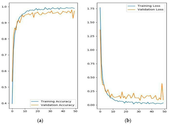
Figure 4. The evolutionary curves of the DCNN-based model over 50 epochs. (a) Training and validation accuracy; (b) training and validation loss.

5.1.2. Accuracy of the Proposed Model Compared with the Accuracy of Other Classical Machine Learning Algorithms

To highlight the higher performance and greater advantages of the proposed DCNN-based model compared with other classical machine learning models, we also trained $K$-nearest neighbors (KNN), support vector machine (SVM), decision tree, and naive Bayes (NB) classifiers, with all parameters configured to the default settings in scikit-learn of Python. An obvious disadvantage of these classical machine learning models lies in the requirement to manually design and extract discriminative features before classification. Therefore, we chose nine common image discriminative features for these classifiers, as shown in Table 4, where Mean Gray, Gray Variance, and Skewness are three gray features; Contrast, Correlation, ASM, Homogeneity, Dissimilarity, and Entropy are six texture features, with each corresponding to four eigenvalues in four directions of 0°, 45°, 90°, and 135°, which reflect the gray distribution, information quantity, and texture thickness of the image from different angles. In total, 27 discriminative features were chosen. Details of the expression for each feature can be seen in the last column of Table 4, where $N$ represents the size of the image, namely, the total number of rows and columns of pixels; $i$ represents the position of the row where the pixel is located; $j$ represents the position of the column where the pixel is located; $p_{(i,j)}$ represents gray value of the pixel at the position of $i$th row and $j$th column; $\theta$ represents four directions of 0°, 45°, 90°, and 135°; and $d$ represents distance between the central pixel and adjacent pixel. In this experiment, $N=512$, $i=0,1,\cdots ,511$, $j=0,1,\cdots ,511$, and $p_{(i,j)}\in \left[0,255\right]$.

In contrast, the DCNN-based model does not require any extra work for designing and extracting features. The detailed results for the DCNN-based model and the above classical models are shown in Table 5. In this study, the evaluation criteria were the highest accuracy, the lowest accuracy, the mean accuracy, and the variance of the accuracies from 10-fold cross-validation. It can be seen that, regardless of the evaluation criterion used, the DCNN-based model was the best. The mean accuracy of the DCNN-based model was 2.5 times that of NB and 1.7 times that of decision tree; in other words, the DCNN-based model had the highest accuracy of the tested models. In addition, the accuracy variance of the DCNN-based model was the smallest: it was three orders of magnitude lower than that of KNN and one order of magnitude lower than that of the other models. That is, the DCNN-based model had the most stable performance of the tested models.

The experimental results also show that the classical machine learning models depend largely on features selected by experts beforehand to increase accuracy [26], whereas the DCNN-based model is able to not only automatically extract the best discriminative features from multiple dimensions, but also learns features layer by layer from low-level features (such as edges, corners, and color) to high-level semantic features (such as shape and object). These capabilities improve the model’s recognition performance on apple cultivar leaf images [26].

From the above two experimental results, we can conclude that the DCNN-based model proposed in this paper can successfully classify apple cultivars, achieving a very high mean accuracy of 0.9711 and a very stable and reliable performance with an accuracy variance of 1.1937e-2. Compared with the classification performance of KNN, SVM, decision tree, and naive Bayes machine learning models, the classification performance of the proposed model is superior and has clear advantages over the others.

5.2. Evaluation of the Generalization Performance on an Independent and Identically Distributed Testing Set

5.2.1. Accuracy on an Independent and Identically Distributed Testing Dataset

Generally, it is more scientifically robust and reliable to evaluate or compare the generalization performance of machine learning models by measuring their accuracy on an unknown dataset. For this purpose, the testing set, training set, and validation set should differ from each other and be independent and identically distributed. The generalization performance of a model should be comprehensively evaluated by its accuracy $acc$, error $\epsilon (=1-acc)$, and other indicators on the unknown testing set. Therefore, in this study, 5% of the leaf images of each cultivar was randomly selected as the fixed testing set for a total of 620 images, which were unknown to the DCNN-based model. Then, of the 11,815 leaf images remaining after excluding the testing set, 90% of the data were chosen at random to form the training set, and the remaining 10% formed the validation set, as detailed in Table 6. The DCNN-based model proposed in this study was trained over 50 epochs on these images using 10-fold cross-validation. The classification results and accuracy ${acc}_i(i=1,2,\dots ,10)$, error ${\epsilon }_i(i=1,2,\dots ,10)$, mean accuracy ${\mu }_{acc}={\displaystyle \sum _{i=1}^n{acc}_i}$, mean error ${\mu }_{\epsilon }={\displaystyle \sum _{i=1}^n{\epsilon }_i}$, and error variance ${\sigma }^2=\frac{1}{n-1}{\displaystyle \sum _{i=1}^n{({\epsilon }_i-{\mu }_{\epsilon })}^2}$ on the fixed unknown independent testing set are shown in Table 7, in which the rows represent the 14 apple cultivars (the number of leaf images for the cultivar is in parentheses), and the columns represent the 10 folds of the cross-validation test. The number of accurately predicted images for each of the 14 apple cultivars in each fold is presented in detail in Table 8, in which with the third-last row represents the accuracy ${acc}_i(i=1,2,\dots ,10)$ of each fold, the second-last row represents the error ${\epsilon }_i(i=1,2,\dots ,10)$ of each fold, the bottom row reports the mean accuracy ${\mu }_{acc}$, mean error ${\mu }_{\epsilon }$, and error variance ${\sigma }^2$ of the 10 folds. The numbers in bold indicate the leaf images classified with 100% accuracy.

Table 6. Testing set, training set, and validation set.

Class	Testing Set	Training Set	Validation Set
2001	47	809	90
ACE	47	802	89
ADR	50	881	98
FJMM	49	840	93
HANF	39	664	74
HRYX	39	666	74
JN1	41	698	78
JAZ	38	648	72
HOC	45	769	85
PIN	44	752	83
JONG	44	759	84
SHF3	50	870	97
GOS	38	646	72
YANF3	49	830	92
Total	620	10,634	1181

Table 7. Accuracy on the testing set.

Class	10-Fold Cross-Validation Tests
	1st	2nd	3rd	4th	5th	6th	7th	8th	9th	10th
2001 (47)	45	46	47	47	46	46	41	47	44	46
ACE (47)	45	47	47	47	47	47	47	47	46	47
ADR (50)	50	50	50	50	50	50	50	50	50	49
FJMM (49)	48	49	45	46	48	47	49	47	47	45
HANF (39)	38	38	29	38	39	37	35	39	36	37
HRYX (39)	37	39	39	37	39	39	38	39	39	39
JN1 (41)	40	37	41	41	40	39	34	38	35	36
JAZ (38)	38	38	38	38	38	38	38	38	38	38
HOC (45)	44	44	42	45	45	42	44	45	43	45
PIN (44)	41	44	41	43	44	42	41	41	44	39
JONG (44)	44	41	44	44	42	44	43	44	44	43
SHF3 (50)	48	47	48	47	47	47	49	47	47	47
GOS (38)	38	38	29	38	38	37	37	38	38	37
YANF3 (49)	48	49	42	46	48	45	49	46	48	46
$acc$	0.9742	0.9790	0.9387	0.9790	0.9855	0.9677	0.9597	0.9774	0.9661	0.9581
$\epsilon$	0.0258	0.0210	0.0613	0.0210	0.0145	0.0323	0.0403	0.0226	0.0339	0.0315
${\mu }_{acc}=0.9716$	${\mu }_{\epsilon }=0.0284$					${\sigma }^2=1.89025E-4$

Table 8. Confusion matrix of the classification results in our work.

	2001	ACE	ADR	FJMM	HANF	HRYX	JN1	JAZ	HOC	PIN	JONG	SHF3	GOS	YANF3
2001	46	0	0	1	0	0	0	0	0	0	0	0	0	0
ACE	0	47	0	0	0	0	0	0	0	0	0	0	0	0
ADR	1	0	49	0	0	0	0	0	0	0	0	0	0	0
FJMM	1	0	0	45	1	0	0	0	0	0	0	1	0	1
HANF	0	0	0	0	37	0	0	0	0	0	0	0	0	2
HRYX	0	0	0	0	0	39	0	0	0	0	0	0	0	0
JN1	0	0	0	0	1	0	36	0	0	0	0	4	0	0
JAZ	0	0	0	0	0	0	0	38	0	0	0	0	0	0
HOC	0	0	0	0	0	0	0	0	45	0	0	0	0	0
PIN	0	0	0	0	0	0	0	0	3	39	2	0	0	0
JONG	1	0	0	0	0	0	0	0	0	0	43	0	0	0
SHF3	0	0	0	0	0	0	0	0	0	0	0	47	0	3
GOS	1	0	0	0	0	0	0	0	0	0	0	0	37	0
YANF3	0	0	0	0	0	0	0	0	0	0	0	3	0	46

As reported in Table 7, for the Jazz cultivar, all 10 folds reached 100% accuracy (highlighted in yellow); for the Ada Red cultivar, nine folds reached 100% accuracy (highlighted in blue); for the Ace cultivar, eight folds reached 100% accuracy (highlighted in green); and for the Hongrouyouxi, Jonagold, and Gold Spur cultivars, more than six folds reached 100% accuracy. Collectively, the mean accuracy ${\mu }_{acc}=0.9685$, mean error ${\mu }_{\epsilon }=0.0315$, and their variance ${\sigma }^2$ = 1.89025E-4 show that the generalization accuracy and stability of the proposed DCNN-based model were very good on the unknown independent testing set.

5.2.2. Test for the General Error of the DCNN-Based Model on an Unknown Testing Set

Ten errors of the DCNN-based model on the unknown independent testing set (Table 7) are in line with the normal distribution, and they can be regarded as independent samples of the generalization error ${\epsilon }_0$, as defined in Equation (6):

$${\tau }_t=\frac{\sqrt{k}({\mu }_{\epsilon }-{\epsilon }_0)}{\sigma }$$

(6)

where ${\tau }_t$ obeys the $t$ distribution for $k-1$ degrees of freedom, as shown in Figure 5 ($k=10,significan\alpha =0.05$):

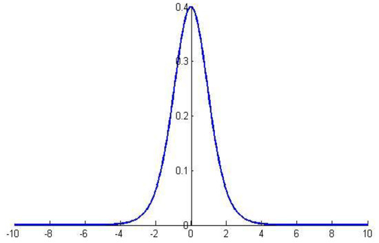
Figure 5. Graph of the $t$ distribution.

For the hypothesis “${\mu }_{\epsilon }={\epsilon }_0$” and significance $\alpha$, we can calculate the maximum error as the critical value that can be observed with a probability of $1-\alpha$ when the mean error is ${\epsilon }_0$. If $\left|\mu -{\epsilon }_0\right|$ is within the range of the critical value [$t_{\frac{-\alpha }{2}},t_{\frac{\alpha }{2}}$], then the hypothesis “${\mu }_{\epsilon }={\epsilon }_0$” cannot be rejected, (i.e., the generalization error is ${\epsilon }_0$, and the confidence degree is $1-\alpha$); otherwise, the hypothesis can be rejected.

The hypothesis “${\mu }_{\epsilon }(=0.0315)={\epsilon }_0$” with significance $\alpha =0.05$ was $t$-tested bilaterally. The critical value calculated in MATLAB r2010a was 2.262, the associated probability was 0.8025, and the confidence interval of the mean error was [0.0209,0.0399]. The results show that the associated probability is far greater than the significance $\alpha =0.05$, so the hypothesis cannot be rejected: that is, the generalization error ${\epsilon }_0$ of the model can be regarded as 0.0315.

5.2.3. Evaluation of Classification Performance in Each Cultivar

The confusion matrix of the classification results on the unknown independent testing set is shown in Table 8. The 14 rows refer to the 14 apple cultivars, and the columns represent the resulting cultivars to which the analyzed leaves were attributed by the proposed DCNN-based model. The fraction of accurately classified images for each apple cultivar is presented in bold on the diagonal in Table 8. As the leaves of Ace, Hongrouyouxi, Jazz, and Honey Crisp cultivars have morphological characteristics that are very prominent and different from the others, the identification rates for these cultivars were 100% (highlighted in yellow). For the 2001, Ada Red, Jonagold, and Gold Spur cultivars, only one leaf was incorrectly identified, and their identification rates were 97.87%, 98%, 97.73%, and 97.37%, respectively. As the leaves of Jingning 1 and Pinova cultivars are similar to the others and lack prominent unique characteristics, the identification rates for these cultivars were the lowest of the 14 cultivars, with values of 87.80% and 88.64%, respectively. Furthermore, we can see mutual equivalent morphological similarities between some cultivars. In fact, for some pairs of cultivars, the number of leaves misclassified for one cultivar was equal to the number of misclassified leaves for the other cultivar and vice versa (highlighted in blue). This was particularly evident for the cultivar pair Shoufu 3 and Yanfu 3: three leaves were wrongly attributed to the other cultivar. An analogous relationship was discovered between the 2001 cultivar (one leaf was wrongly attributed to the Fujimeiman cultivar) and the Fujimeiman cultivar (one leaf was wrongly identified as the 2001 cultivar). Furthermore, although the accuracy for the Fujimeiman cultivar was not the lowest, four of its leaves were not correctly identified and broadly misclassified as four different cultivars. All of these interesting results offer important insights and inspirations that breeding experts can apply in their work for the selection of new apple varieties.

The specific parameters that define the classification accuracy for each cultivar are the true positive $TP$, false positive $FP$, true negative $TN$, and false negative $FN$ [21], as detailed below.

The $TP$ rate $TPR=\frac{TP}{TP+FN}$, also known as sensitivity, measures the proportion of positives that are correctly classified as such, in machine learning, the $TP$ rate is also known as the probability of detection [24]. The $TN$ rate $TNR=\frac{TN}{FP+TN}$, also known as specificity, measures the proportion of negatives that are correctly identified as such. The $FP$ rate $FPR=\frac{FP}{FP+TN}$, also known as the fall-out or probability of false alarm [24], measures the proportion of positives that are incorrectly identified as negatives, can also be calculated as “1 − specificity”. The accuracy rate $A=\frac{TP+TN}{TP+FP+TN+FN}$ measures the proportion of positives and negatives that are correctly identified as such; Precision $P=\frac{TP}{TP+FP}$ measures the correctly identified proportion of positives; and Recall $R=\frac{TP}{TP+FN}$ measures the correctly identified proportion of positives that are identified as such. $F_{\beta \_\mathrm{score}}=\frac{(1+{\beta }^2)*P*R}{{\beta }^2*P+R}$, known as the harmonic mean of $P$ and $R$, measures the preference of attention on Precision or Recall: when $\beta >1$, $R$ receives more attention than $P$ and vice versa; in this study, $\beta =1$. The macro accuracy rate $A_{\mathrm{macro}}=\frac{1}{n}{\displaystyle \sum _{i=1}^n{A}_i}$, macro Precision $P_{\mathrm{macro}}=\frac{1}{n}{\displaystyle \sum _{i=1}^n{P}_i}$, macro Recall $R_{\mathrm{macro}}=\frac{1}{n}{\displaystyle \sum _{i=1}^n{R}_i}$, and macro $F_{\beta \_\mathrm{score}}^{\mathrm{macro}}=\frac{(1+{\beta }^2)*P_{\mathrm{macro}}*R_{\mathrm{macro}}}{{\beta }^2*P_{\mathrm{macro}}+R_{\mathrm{macro}}}$ were used to measure the global average performance of the DCNN-based model on the 14 cultivars in the testing set. The detailed accuracy of the DCNN model for each apple cultivar is shown in Table 9. The values of $R(=TPR)$ for ACE, ADR, HRYX, JAZ, and HOC cultivars were greater than 0.98, and only the values of $R(=TPR)$ for the JN1 and PIN cultivars were less than 0.90. Additionally, $R_{\mathrm{macro}}=0.9586$, which illustrates that the DCNN-based model was sensitive for each cultivar, and the $TNR$ of each cultivar was nearly equal to 1, which demonstrates that the DCNN-based model had excellent specificity. The $FPR$ was below 0.005 for 12 cultivars; thus, the fall-out or probability of false alarm of the DCNN-based model was perfect for 86% of the cultivars. The accuracy rate of each cultivar was sufficiently high—above 0.98 for all cultivars—and $A_{\mathrm{macro}}=0.9940$: in other words, when leaves are mixed together, if we want to distinguish a specific cultivar’s leaves from the others, the DCNN-based model can absolutely correctly identify the leaves that belong to a specific cultivar and the leaves that do not belong to it, with such identified leaves accounting for 99.40% of the total number leaves. Only the values of Precision $P$ for Shoufu 3 and Yanfu 3 cultivars were slightly lower than 0.92, and the other cultivars were identified with high precision, as reflected by $P_{\mathrm{macro}}=0.9628$, which indicates that the model had a high precision for most of the cultivars. For the $F_{\beta \_\mathrm{score}}^{}$ of the cultivars, with $F_{\beta \_\mathrm{macro}}^{}=0.9607$, we can draw the same conclusion as that for Precision $P$.

Table 9. Accuracy for each cultivar.

Class	$\mathit{T}\mathit{P}$	$\mathit{F}\mathit{P}$	$\mathit{F}\mathit{N}$	$\mathit{T}\mathit{N}$	$\mathit{T}\mathit{P}\mathit{R}$	$\mathit{T}\mathit{N}\mathit{R}$	$\mathit{F}\mathit{P}\mathit{R}$	$\mathit{A}$	$\mathit{P}$	$\mathit{R}$	${\mathit{F}}_{\mathit{\beta }\_\mathbf{score}}^{}$
2001	46	4	1	569	0.9787	0.9930	0.0070	0.9919	0.9200	0.9787	0.9485
ACE	47	0	0	573	1.0000	1.0000	0.0000	1.0000	1.0000	1.0000	1.0000
ADR	49	0	1	570	0.9800	1.0000	0.0000	0.9984	1.0000	0.9800	0.9899
FJMM	45	1	4	570	0.9184	0.9982	0.0018	0.9919	0.9783	0.9184	0.9474
HANF	37	2	2	579	0.9487	0.9966	0.0034	0.9935	0.9487	0.9487	0.9487
HRYX	39	0	0	581	1.0000	1.0000	0.0000	1.0000	1.0000	1.0000	1.0000
JN1	36	0	5	579	0.8780	1.0000	0.0000	0.9919	1.0000	0.8780	0.9351
JAZ	38	0	0	582	1.0000	1.0000	0.0000	1.0000	1.0000	1.0000	1.0000
HOC	45	3	0	572	1.0000	0.9948	0.0052	0.9952	0.9375	1.0000	0.9677
PIN	39	0	5	576	0.8864	1.0000	0.0000	0.9919	1.0000	0.8864	0.9398
JONG	43	2	1	574	0.9773	0.9965	0.0035	0.9952	0.9556	0.9773	0.9663
SHF3	47	8	3	562	0.9400	0.9860	0.0140	0.9823	0.8545	0.9400	0.8952
GOS	37	0	1	582	0.9737	1.0000	0.0000	0.9984	1.0000	0.9737	0.9867
YANF3	46	6	3	565	0.9388	0.9895	0.0105	0.9855	0.8846	0.9388	0.9109
$A_{\mathrm{macro}}=0.9940$			$P_{\mathrm{macro}}=0.9628$			$R_{\mathrm{macro}}=0.9586$			$F_{\beta \_\mathrm{macro}}^{}=0.9607$

Hence, from all the above experiments, we can conclude that the DCNN-based model proposed in this paper achieved a high enough performance on each cultivar, except for the Shoufu 3 and Yanfu 3 cultivars, mainly because of the highly similar morphological traits shared between this pair of cultivars. The genetic relationship between the Shoufu 3 and Yanfu 3 cultivars is very high. Both were selected from a red mutation of Fuji and bred in Yantai City, Shandong Province, China. The passport details for these two cultivars are in Table 10.

Table 10. Passports for the Shoufu 3 and Yanfu 3 cultivars.

Class	Platform No.	Resource No.	Origin	Type
SHF3	1111C0003883000057	MAPUM6208260057	Xiaocaogou Horticultural farm of Laizhou, Yantai City, Shandong Province	Breeding variety
YANF 3	1111C0003883000006	MAPUM6208260006	Fruit and Tea Extension Station of Yantai, Yantai City, Shandong Province	Breeding variety

From the National Forest Germplasm Resources Platform of China.

6. Conclusions

This paper proposes a novel approach to identify apple cultivars using a deep convolution neural network with leaf image input. No extra work is required for designing and extracting discriminative features, and it can automatically discover semantic features at different depths and enable an end-to-end learning pipeline with high accuracy. To provide sufficient apple cultivar leaf images for training the model to obtain high generalization performance, we captured the images of apple leaves in the orchard under natural sunlight conditions at a resolution of 3264 × 2448 and/or 1600 × 1200 from multiple angles in the automatic shooting mode. In particular, two main factors were considered to increase the diversity of the leaf images: first, 1481 leaves were randomly picked from the branches at the periphery and the inner bore in four directions (east, west, south, and north) of the tree crown; second, the leaf images were captured over a period of 37 days, from 15 July 2019 to 20 August 2019, during which the weather conditions were variable. Finally, a total of 12,435 leaf images for 14 apple cultivars were obtained. Furthermore, by analyzing the characteristics of apple cultivar leaves, a novel model structure was designed by (i) setting all the convolution kernels to the same size of 3 * 3 to prevent the loss of important features and to simplify the model; (ii) adding a max-pooling operation after each convolution layer to reduce the amount of computation; and (iii) introducing the dropout operation after the dense layer to prevent the model from over-fitting.

The DCNN-based model was implemented in the TensorFlow framework on a GPU platform. The test results on a dataset of 12,435 leaf images from 14 cultivars show that the proposed model, with a mean accuracy of 0.9711 on 14 apple cultivars, is much better than several traditional models. Its evolutionary curves show that the model effectively overcomes the over-fitting problem. Furthermore, we performed comparative experiments to test the accuracy of the DCNN-based model on an unknown independent dataset, and the mean accuracy, the mean error, and their variance were ${\mu }_{acc}=0.9685$, ${\mu }_{\epsilon }=0.0315$, and ${\sigma }^2$ = 1.89025E-4, respectively, which show that the generalization accuracy and stability of the model proposed in this paper were very good on the unknown independent testing set. Finally, we analyzed and compared the performance of the model on each cultivar in the unknown independent dataset, and the results showed that an accuracy of 100.00% was achieved for the b, f, h, and i cultivars, and only one leaf was incorrectly identified for the a, c, k, and m cultivars, with accuracies of 0.9787, 0.9800, 0.9773, and 0.9737, respectively. The lowest accuracies were obtained for the g and j cultivars, with 0.8780 and 0.8864, respectively. Finally, TPR = 0.9685, FPR = 0.0024, and TNR = 0.9976 collectively indicate that the model generally has high precision and recall performance.

Future work will aim to identify apple cultivars in real time by studying other deep neural network models such as Faster RCNN (Regions with Convolutional Neural Network), YOLO (You Only Look Once), and SSD (Single Shot MultiBox Detector). Furthermore, hundreds and thousands of leaf images of more apple cultivars from different planting areas need to be gathered to increase the generalization performance and efficiency of the model on more apple cultivars. This presented model will also be used to identify other fruit tree cultivars and even other plants.

References

- Srivastava, K.K.; Ahmad, N.; Das, B.; Sharma, O.C.; Singh, S.R.; Rather, J.A. Genetic divergence in respect to qualitative traits and their possible use in precision breeding programme of apple (Malus Domestica). Indian J. Agric. Sci. 2013, 83, 1217–1220. [Google Scholar]
- Peihua, C. Apple Varieties in China[M]; China Agriculture Press: Beijing, China, 2015; pp. 2–6. [Google Scholar]
- Zhengyang, Z. Fruit Science and Practice in China. Apple[M]; Shaanxi Science and Technology Press: Xi’an, China, 2015; pp. 1–7. [Google Scholar]
- Sheth, K. 25 Countries That Import The Most Apples. WorldAtlas. Available online: https://www.worldatlas.com/articles/the-countries-with-the-most-apple-imports-in-the-world.html (accessed on 25 December 2019).
- Sohu News. “World Apple Production and Sales in 2018/2019.”. Available online: https://www.http://www.sohu.com/a/284046969_120045201 (accessed on 12 December 2019).
- Chen, X.S.; Han, M.Y.; Su, G.L.; Liu, F.Z.; Guo, G.N.; Jiang, Y.M.; Mao, Z.Q.; Peng, F.T.; Shu, H.R. Discussion on today’s world apple industry trends and the suggestions on sustainable and efficient development of apple industry in China. J. Fruit Sci. 2010, 27, 598–604. [Google Scholar]
- Lixin, W.; Xiaojun, Z. Establishment of SSR fingerprinting database on major apple cultivars. J. Fruit Sci. 2012, 29, 971–977. [Google Scholar]
- Huiling, M.; Wang, R.; Cheng, C.; Dong, W. Rapid Identification of Apple Varieties Based on Hyperspectral Imaging. Trans. Chin. Soc. Agric. Mach. 2017, 48, 305–312. [Google Scholar]
- Ba, Q.; Zhao, Z.; Gao, H.; Wang, Y.; Sun, B. Genetic Relationship Analysis of Apple Cultivars Using SSR and SRAP Makers. J. Northwest A F Univ. -Nat. Sci. Ed. 2011, 39, 123–128. [Google Scholar]
- Hongjie, S. Identification of Grape Varieties Based on Leaves Image Analysis; Northwest A&F University: Xianyang, China, 2016. [Google Scholar]
- Pankaja, K.; Suma, V. Leaf Recognition and Classification Using Chebyshev Moments. In Smart Intelligent Computing and Applications; Smart Innovation, Systems and Technologies; Satapathy, S., Bhateja, V., Das, S., Eds.; Springer: Singapore, 2019; Volume 105. [Google Scholar]
- Hall, D.; McCool, C.; Dayoub, F.; Sunderhauf, N.; Upcroft, B. Evaluation of Features for Leaf Classification in Challenging Conditions. In Proceedings of the 2015 IEEE Winter Conference on Applications of Computer Vision, WACV, Waikoloa, HI, USA, 5–9 January 2015; pp. 797–804. [Google Scholar] [CrossRef]
- Söderkvist, O. Computer Vision Classification of Leaves from Swedish Trees. Master’s Thesis, Teknik Och Teknologier, Stockholm, Sweden, 2001. [Google Scholar]
- Lei, W.; Dongjian, H.; Yongliang, Q. Study on plant leaf classification based on image processing and SVM. J. Agric. Mech. Res. 2013, 5, 12–15. [Google Scholar]
- Zhang, S.; Ju, C. Orthogonal global-locally discriminant projection for plant leaf classification. Nongye Gongcheng Xuebao/Trans. Chin. Soc. Agric. Eng. 2010, 26, 162–166. [Google Scholar]
- Dyrmann, M.; Karstoft, H.; Midtiby, H.S. Plant species classification using deep convolutional neural network. Biosyst. Eng. 2016, 151, 72–80. [Google Scholar] [CrossRef]
- Yalcin, H.; Razavi, S. Plant classification using convolutional neural networks. In Proceedings of the 5th International Conference on Agro-geoinformatics, Tianjin, China, 18–20 July 2016; pp. 1–5. [Google Scholar]
- Lee, S.H.; Chan, C.S.; Remagnino, P. Multi-Organ Plant Classification Based on Convolutional and Recurrent Neural Networks. IEEE Trans. Image Process. 2018. [Google Scholar] [CrossRef] [PubMed]
- ImageCLEF / LifeCLEF—Multimedia Retrieval in CLE. Available online: https://www.imageclef.org/2015 (accessed on 16 September 2019).
- Sue, H.L.; Chee, S.C.; Simon, J.M.; Paolo, R. How deep learning extracts and learns leaf features for plant classification. Pattern Recognit. 2017, 71, 1–13. [Google Scholar]
- Guillermo, L.G.; Lucas, C.U.; Mónica, G.L.; Pablo, M.G. Deep learning for plant identification using vein morphological patterns. Comput. Electron. Agric. 2016, 127, 418–424. [Google Scholar]
- Baldi, A.; Pandolfi, C.; Mancuso, S.; Lenzi, A. A leaf-based back propagation neural network for oleander (Nerium oleander L.) cultivar identification. Comput. Electron. Agric. 2017, 142, 515–520. [Google Scholar] [CrossRef]
- Weather China. Available online: https://www.weather.com.cn (accessed on 20 August 2019).
- MATLAB for Artificial Intelligence. Available online: www.mathworks.com (accessed on 10 November 2019).
- Hanson, A.M.J.; Joy, A.; Francis, J. Plant leaf disease detection using deep learning and convolutional neural network. Int. J. Eng. Sci. Comput. 2017, 7, 5324–5328. [Google Scholar]
- Lu, Y.; Yi, S.J.; Zeng, N.Y.; Liu, Y.; Zhang, Y. Identification of rice diseases using deep convolutional neural networks. Neurocomputing 2017, 267, 378–384. [Google Scholar] [CrossRef]
- Kawasaki, Y.; Uga, H.; Kagiwada, S.; Iyatomi, H. Basic study of automated diagnosis of viral plant diseases using convolutional neural networks. In Proceedings of the 12th International Symposium on Visual Computing, Las Vegas, NV, USA, 12–14 December 2015; pp. 638–645. [Google Scholar]
- Mohanty, S.P.; Hughes, D.P.; Marcel, S. Using deep learning for image-based plant disease detection. Front. Plant Sci. 2016, 7, 14–19. [Google Scholar] [CrossRef] [PubMed]
- Fuentes, A.; Yoon, S.; Kim, S.C.; Park, D.S. A robust deep-learning-based detector for real-time tomato plant diseases and pests recognition. Sensors 2017, 17, 2022. [Google Scholar] [CrossRef] [PubMed]
- Sladojevic, S.; Arsenovic, M.; Anderla, A.; Culibrk, D.; Stefanovic, D. Deep neural networks based recognition of plant diseases by leaf image classification. Comput. Intell. Neurosci. 2016, 2016. [Google Scholar] [CrossRef] [PubMed]
- Liu, B.; Zhang, Y.; He, D.; Li, Y. Identification of Apple Leaf Diseases Based on Deep Convolutional Neural Networks. Symmetry 2018, 10, 11. [Google Scholar] [CrossRef]
© 2020 by the authors. Licensee MDPI, Basel, Switzerland. This article is an open access article distributed under the terms and conditions of the Creative Commons Attribution (CC BY) license (http://creativecommons.org/licenses/by/4.0/).