Soliton Behaviours for the Conformable Space–Time Fractional Complex Ginzburg–Landau Equation in Optical Fibers

Abstract

In this work, we investigate the conformable space–time fractional complex Ginzburg–Landau (GL) equation dominated by three types of nonlinear effects. These types of nonlinearity include Kerr law, power law, and dual-power law. The symmetry case in the GL equation due to the three types of nonlinearity is presented. The governing model is dealt with by a straightforward mathematical technique, where the fractional differential equation is reduced to a first-order nonlinear ordinary differential equation with solution expressed in the form of the Weierstrass elliptic function. The relation between the Weierstrass elliptic function and hyperbolic functions enables us to derive two types of optical soliton solutions, namely, bright and singular solitons. Restrictions for the validity of the optical soliton solutions are given. To shed light on the behaviour of solitons, the graphical illustrations of obtained solutions are represented for different values of various parameters. The symmetrical structure of some extracted solitons is deduced when the fractional derivative parameters for space and time are symmetric.

1. Introduction

The optical solitons have become an important research topic in the physical and natural sciences. It has been found that solitons play a significant role in various branches of science, such as optical fibres, plasma physics, nonlinear optics, and many other fields [1,2,3,4,5]. In fibre optics, for instance, solitons can propagate along trans-continental and trans-oceanic distances. Understanding the dynamics of solitons can lead to interpret the physics of phenomena in which they exist. Thus, a variety of powerful mathematical approaches have been developed to derive soliton solutions for many physical models. For more details, readers are referred to references [6,7,8,9,10,11,12,13,14,15,16,17,18,19,20].

Recently, the study of physical models with fractional derivatives has attracted a great deal of attention since some materials are well described as fractal media. To investigate such models, several definitions of fractional derivatives such as Caputo [21], Caputo–Fabrizio [22], Riemann–Liouville [23], and Grünwald–Letnikov [24] have been introduced. It is found that fractional derivatives do not satisfy some basic properties of derivatives, such as the product rule and chain rule. Recently, Khalil et al. [25] developed a local derivative called a conformable derivative where this fractional calculus satisfies all the properties of derivatives like the chain rule.

The present study sheds light on the space–time fractional complex Ginzburg–Landau (GL) equation [26,27]. The GL model addressed here is described by

$$i{D}_t^{\alpha }\mathsf{\Psi }+a{D}_x^{2\beta }\mathsf{\Psi }+{bF(|\mathsf{\Psi }|}^2)\mathsf{\Psi }-{\left({\left|\mathsf{\Psi }\right|}^2{\mathsf{\Psi }}^{*}\right)}^{-1}\left[{\nu \left|\mathsf{\Psi }\right|}^2{D}_x^{2\beta }{(|\mathsf{\Psi }|}^2)-\varrho {\left(D_x^{\beta }{(|\mathsf{\Psi }|}^2)\right)}^2\right]-\gamma \mathsf{\Psi }=0,$$

(1)

where $\alpha$ and $\beta$ are the fractional parameters. The complex-valued function $\mathsf{\Psi }(x,t)$ denotes the soliton profile whereas the independent variables x and t are the spatial and temporal coordinates. Here, a and b stand for the coefficient of group velocity dispersion and the coefficient of nonlinearity, respectively. The real-valued constants $\nu ,\varrho ,\gamma$ represent the perturbation influences. The symbol ∗ indicates the complex conjugate of the function $\mathsf{\Psi }(x,t)$.

Note that the travelling wave reduction of the GL model (1) is obtained by taking $\nu =2\varrho$ in all previous studies [26,27,28,29,30,31,32,33,34,35,36,37,38]. Then, the analytic exact solution is extracted by applying various integration schemes (first integral method, semi-inverse variational principle, $G^{\prime }/G$ method, exp-function method, Riccati equation method, simplest equation method, trial solution approach, etc.). Recently, Equation (1) with Kerr law nonlinearity was studied by [27] using the same assumption (i.e., $\nu =2\varrho$). The extended sinh-Gordon equation expansion method is employed to derive optical solitons and other solutions. In the current article, we investigate two types of solitons called the bright and singular optical solitons of Equation (1) by means of a straightforward mathematical approach. We discuss three types of nonlinearity associating with the GL Equation (1), which are the Kerr law, power law, and dual-power law. Contrary to the previous studies, herein we will consider $a=4\varrho$ instead of $\nu =2\varrho$. The aim of this assumption is to present the difference between the behaviour of solitons derived here and in the previous studies.

2. Conformable Fractional Derivative

A new form of conformable fractional derivative was introduced by Khalil et al. [25]. This new definition of fractional calculus is based on a limit operator which is more natural and effective in satisfying some conventional properties than the existing fractional derivatives. The definition of a conformable fractional derivative is given as follows:

Definition 1.

Let $f:(0,\infty )⟶R$, then the conformable fractional derivative of f of order α is defined as

$$D_t^{\alpha }f(t)=\underset{ϵ\to 0}{lim}\frac{f(t+ϵt^{1-\alpha })-f(t)}{ϵ},$$

(2)

for all $t>0,\alpha \in (0,1)$. It is said that if the conformable fractional derivative of f of order α exists, then f is α-differentiable.

The conformable fractional derivative satisfies the properties shown in the following theorems:

Theorem 1.

Let $\alpha \in (0,1]$ and $f=f(t),g=g(t)$ be α-differentiable at a point $t>0$, then:

$$\begin{array}{cc}(1)& D_t^{\alpha }(af+bg)=a{D}_t^{\alpha }f+b{D}_t^{\alpha }g,foralla,b\in R.\hfill \\ (2)& D_t^{\alpha }(t^{\mu })=\mu t^{\mu -\alpha },forall\mu \in R.\hfill \\ (3)& D_t^{\alpha }(fg)=f{D}_t^{\alpha }g+g{D}_t^{\alpha }f.\hfill \\ (4)& D_t^{\alpha }\left(\frac{f}{g}\right)=\frac{g{D}_t^{\alpha }f-f{D}_t^{\alpha }g}{g^2}.\hfill \end{array}$$

Moreover, if f is differentiable, then $D_t^{\alpha }(f(t))=t^{1-\alpha }\frac{\mathrm{d}f}{\mathrm{d}t}$.

Theorem 2.

Let $f:(0,\infty )⟶R$ be a function such that f is differentiable and also α-differentiable. Let g be a function defined in the range of f and also differentiable; then, one has the following rule:

$$D_t^{\alpha }(fg)(t)=t^{1-\alpha }{g}^{\prime }(t)f^{\prime }(g(t)),$$

(3)

where prime denotes the classical derivatives with respect to t.

Remark 1.

We may use the notation $\frac{{\partial }^{\alpha }}{\partial t^{\alpha }}f$ for $D_t^{\alpha }(f(t))$ to denote the conformable fractional derivatives of f with respect to the variable t of order α.

3. Mathematical Analysis and Equations

In this section we describe the technique of reducing FDEs into ordinary differential equations (ODEs). Then, this method will be implemented to obtain the travelling wave reduction for the governing model (1) in order to extract exact analytic solutions.

3.1. Description of the Method

Suppose that a nonlinear conformable fractional partial differential equation, say, in two independent variables x and t, is given by

$$P(u,D_t^{\alpha }u,D_x^{\beta }u,D_t^{2\alpha }u,D_x^{2\beta }u,D_x^{\beta }{D}_t^{\alpha }u,\dots )=0,$$

(4)

where $u(x,t)$ is an unknown function, P is a polynomial in u and its partial derivatives, in which the highest-order derivatives and nonlinear terms are involved.

Using the wave transformation

$$u(x,t)=U(\xi ),\xi =k\frac{x^{\beta }}{\beta }+c\frac{t^{\alpha }}{\alpha },$$

(5)

where k and c are constants to be determined later, one can find

$$D_t^{\alpha }u=c{U}^{\prime },D_x^{\beta }u=k{U}^{\prime },D_t^{2\alpha }u=c^2{U}^{″},D_x^{2\beta }u=k^2{U}^{″},D_x^{\beta }{D}_t^{\alpha }u=kc{U}^{″},\cdots$$

(6)

Employing (5) and (6), Equation (4) is reduced to the following ODE

$$P(U,c{U}^{\prime },k{U}^{\prime },c^2{U}^{″},k^2{U}^{″},kc{U}^{″},\cdots )=0,$$

(7)

where prime (${}^{\prime }$) denotes the derivative with respect to $\xi$.

3.2. Travelling Wave Reduction for Equation (1)

Consider the complex fractional travelling wave transformation

$$\mathsf{\Psi }(x,t)=\psi (\xi )e^{i\varphi (x,t)},$$

(8)

where the wave variable $\xi$ is given by

$$\xi =\frac{x^{\beta }}{\beta }-c\frac{t^{\alpha }}{\alpha },0<\alpha ,\beta \le 1.$$

(9)

The function $\psi (\xi )$ denotes the pulse shape and c is the velocity of the soliton. The phase component is defined as

$$\varphi (x,t)=-k\frac{x^{\beta }}{\beta }-\omega \frac{t^{\alpha }}{\alpha }+\theta ,$$

(10)

where k is the soliton frequency, $\omega$ is the soliton wave number, and $\theta$ is the phase constant.

Using transformation (8), Equation (1) yields a nonlinear ODE of the form

$$(a-2\nu ){\psi }^{″}+(4\varrho -2\nu )\frac{{\psi }^{\prime 2}}{\psi }-(\omega +\gamma +a{k}^2)\psi +bF({\psi }^2)\psi =0,$$

(11)

from the real part and the relation $c=-2ak$ from the imaginary part. All former studies given by references [26,27,28,29,30,31,32,33,34,35,36,37,38] assumed that $\nu =2\varrho$ so as to eliminate the term proportional to ${\psi }^{\prime 2}/\psi$. Thus, Equation (11) becomes

$$(a-2\nu ){\psi }^{″}-(\omega +\gamma +a{k}^2)\psi +bF({\psi }^2)\psi =0.$$

(12)

In contrast to the assumption $\nu =2\varrho$ made by the previous studies, we assume here that $a=4\varrho$. Therefore, Equation (11) is converted to

$$(a-2\nu )({\psi }^{″}+\frac{{\psi }^{\prime 2}}{\psi })-(\omega +\gamma +a{k}^2)\psi +bF({\psi }^2)\psi =0.$$

(13)

In what follows, we aim to derive the soliton solutions of Equation (1) via the study of Equation (13) in the presence of three different laws of nonlinearity. These nonlinear effects include Kerr law, power law and dual-power law.

4. Solitons with Kerr Law Nonlinearity

For the Kerr law nonlinearity, $F(\psi )=\psi$. Hence, Equation (13) has the form

$$(a-2\nu )({\psi }^{″}+\frac{{\psi }^{\prime 2}}{\psi })-(\omega +\gamma +a{k}^2)\psi +b{\psi }^3=0.$$

(14)

Multiplying Equation (14) by ${\psi }^2{\psi }^{\prime }$ and integrating with respect to $\xi$, we arrive, after manipulating, at

$$6(a-2\nu ){\psi }^2{\psi }^{\prime 2}+12c_0-3(\omega +\gamma +a{k}^2){\psi }^4+2b{\psi }^6=0,$$

(15)

where $c_0$ is the integration constant. In order to simplify and solve Equation (15), the following assumption will be used. Setting

$$\psi =\sqrt{V},$$

(16)

one can find that ${\psi }^2{\psi }^{\prime 2}=V^{\prime 2}/4$. Thus, Equation (15) becomes

$$3(a-2\nu )V^{\prime 2}+24c_0-6(\omega +\gamma +a{k}^2)V^2+4b{V}^3=0.$$

(17)

Rearranging Equation (17) so it has the form

$$V^{\prime 2}=-A{V}^3+B{V}^2-C,$$

(18)

where

$$A=\frac{4b}{3(a-2\nu )},B=\frac{6(\omega +\gamma +a{k}^2)}{3(a-2\nu )},C=\frac{24c_0}{3(a-2\nu )}.$$

(19)

Now we will assume that

$$V(\xi )=W(\xi )+\frac{B}{3A}.$$

(20)

Subsequently, Equation (18) reduces to

$$W^{\prime 2}=-A{W}^3+\frac{B^2}{3A}W+\left(\frac{2B^3}{27A^2}-C\right).$$

(21)

Multiplying Equation (21) by $-4/A$ and assuming $Y(\zeta )=W(\xi ),\zeta =\sqrt{-A}\xi /2$, we reach

$$Y^{\prime 2}=4Y^3-g_{2}Y-g_3,$$

(22)

where the prime (${}^{\prime }$) is the derivative with respect to $\zeta$. The invariants $g_2$ and $g_3$ are given by

$$g_2=\frac{4B^2}{3A^2},g_3=\frac{4}{A}\left(\frac{2B^3}{27A^2}-C\right).$$

(23)

It is well known that the general solution of Equation (22) is expressed in terms of Weierstrass elliptic function [39,40] as

$$Y(\zeta )=\wp (\zeta ,g_2,g_3).$$

(24)

Hence, the general solution of Equation (18) reads as

$$V(\xi )=\wp \left(\frac{\sqrt{-A}}{2}\xi ,g_2,g_3\right)+\frac{B}{3A}.$$

(25)

If the discriminant $\mathsf{\Delta }=g_2^3-27g_3^2=0$, this enables us to express Weierstrass elliptic function in the form of hyperbolic functions using the relations

$$\begin{array}{c}\hfill \wp (\zeta ,12r^2,-8r^3)=r-3r{cosh}^{-2}[{(3r)}^{1/2}\zeta ],\end{array}$$

(26)

$$\begin{array}{c}\hfill \wp (\zeta ,12r^2,-8r^3)=r+3r{sinh}^{-2}[{(3r)}^{1/2}\zeta ].\end{array}$$

(27)

In order to extract soliton solutions for Equation (18) using relations (26) and (27), the discriminant $\mathsf{\Delta }=0$ should be satisfied. Therefore

$$\mathsf{\Delta }=g_2^3-27g_3^2=\frac{1}{A^4}(64B^{3}C-432A^2{C}^2)=0,$$

(28)

implies that $C=0$ or $C=4B^3/(27A^2)$.

Case I.$C=0$ demands $g_2=\frac{4B^2}{3A^2}$ and $g_3=\frac{8B^3}{27A^3}$. Thus, solution (25) leads to

$$\begin{array}{c}V(\xi )=\frac{B}{A}{sech}^2\left(\frac{\sqrt{B}}{2}\xi \right),\hfill \end{array}$$

(29)

$$\begin{array}{c}V(\xi )=-\frac{B}{A}{csch}^2\left(\frac{\sqrt{B}}{2}\xi \right),\hfill \end{array}$$

(30)

where $B>0$. As a result, Equation (1) with Kerr law nonlinearity possesses a bright optical soliton solution in the form

$$\mathsf{\Psi }(x,t)=\sqrt{\frac{3(\omega +\gamma +a{k}^2)}{2b}}sech\left(\sqrt{\frac{(\omega +\gamma +a{k}^2)}{2(a-2\nu )}}\left(\frac{x^{\beta }}{\beta }-c\frac{t^{\alpha }}{\alpha }\right)\right)e^{i\left(-k\frac{x^{\beta }}{\beta }-\omega \frac{t^{\alpha }}{\alpha }+\theta \right)},$$

(31)

where $b(\omega +\gamma +a{k}^2)>0$ and $(a-2\nu )(\omega +\gamma +a{k}^2)>0$. Next, Equation (1) admits a singular optical soliton solution in the form

$$\mathsf{\Psi }(x,t)=\sqrt{-\frac{3(\omega +\gamma +a{k}^2)}{2b}}csch\left(\sqrt{\frac{(\omega +\gamma +a{k}^2)}{2(a-2\nu )}}\left(\frac{x^{\beta }}{\beta }-c\frac{t^{\alpha }}{\alpha }\right)\right)e^{i\left(-k\frac{x^{\beta }}{\beta }-\omega \frac{t^{\alpha }}{\alpha }+\theta \right)},$$

(32)

where $b(\omega +\gamma +a{k}^2)<0$ and $(a-2\nu )(\omega +\gamma +a{k}^2)>0$.

Case II.$C=\frac{4B^3}{27A^2}$ demands $g_2=\frac{4B^2}{3A^2}$ and $g_3=-\frac{8B^3}{27A^3}$. Thus, solution (25) gives rise to

$$\begin{array}{c}V(\xi )=\frac{B}{3A}\left[2-3{sech}^2\left(\frac{\sqrt{-B}}{2}\xi \right)\right],\hfill \end{array}$$

(33)

$$\begin{array}{c}V(\xi )=\frac{B}{3A}\left[2+3{csch}^2\left(\frac{\sqrt{-B}}{2}\xi \right)\right],\hfill \end{array}$$

(34)

where $B<0$. Consequently, Equation (1) has singular optical soliton solutions in the form

$$\begin{array}{c}\hfill \mathsf{\Psi }(x,t)=\sqrt{\frac{(\omega +\gamma +a{k}^2)}{2b}\left[2-3{sech}^2\left(\sqrt{-\frac{(\omega +\gamma +a{k}^2)}{2(a-2\nu )}}\left(\frac{x^{\beta }}{\beta }-c\frac{t^{\alpha }}{\alpha }\right)\right)\right]}{e}^{i\left(-k\frac{x^{\beta }}{\beta }-\omega \frac{t^{\alpha }}{\alpha }+\theta \right)},\end{array}$$

(35)

$$\begin{array}{c}\hfill \mathsf{\Psi }(x,t)=\sqrt{\frac{(\omega +\gamma +a{k}^2)}{2b}\left[2+3{csch}^2\left(\sqrt{-\frac{(\omega +\gamma +a{k}^2)}{2(a-2\nu )}}\left(\frac{x^{\beta }}{\beta }-c\frac{t^{\alpha }}{\alpha }\right)\right)\right]}{e}^{i\left(-k\frac{x^{\beta }}{\beta }-\omega \frac{t^{\alpha }}{\alpha }+\theta \right)},\end{array}$$

(36)

with constraint conditions

$$c_0=\frac{{(\omega +\gamma +a{k}^2)}^3}{12b^2},(a-2\nu )(\omega +\gamma +a{k}^2)<0.$$

(37)

5. Solitons with Power Law Nonlinearity

For the power law nonlinearity, $F(\psi )={\psi }^n$. Therefore, Equation (13) has the form

$$(a-2\nu )({\psi }^{″}+\frac{{\psi }^{\prime 2}}{\psi })-(\omega +\gamma +a{k}^2)\psi +b{\psi }^{2n+1}=0.$$

(38)

Multiplying Equation (38) by ${\psi }^2{\psi }^{\prime }$ and integrating with respect to $\xi$, we find the equation

$$2(a-2\nu ){\psi }^2{\psi }^{\prime 2}-(\omega +\gamma +a{k}^2){\psi }^4+\frac{2b}{n+2}{\psi }^{2n+4}=0,$$

(39)

where the integration constant is taken to be zero. Similarly, using assumption (16), Equation (39) changes to the form

$$(a-2\nu )V^{\prime 2}-2(\omega +\gamma +a{k}^2)V^2+\frac{4b}{n+2}{V}^{n+2}=0.$$

(40)

It is obvious that Equation (40) is symmetrical to Equation (17) once $n=1$ and $c_0=0$. Now, setting $V=W^{1/n}$, Equation (40) becomes

$$\frac{(a-2\nu )}{n^2}{W}^{\prime 2}-2(\omega +\gamma +a{k}^2)W^2+\frac{4b}{n+2}{W}^3=0.$$

(41)

Equation (41) can be written as

$$W^{\prime 2}=-A{W}^3+B{W}^2,$$

(42)

where

$$A=\frac{4b{n}^2}{(n+2)(a-2\nu )},B=\frac{2(\omega +\gamma +a{k}^2)n^2}{(a-2\nu )}.$$

(43)

By comparison, the structures of Equation (42) and Equation (18) are symmetric when $C=0$. Therefore, Equation (42) has the solutions of the form

$$\begin{array}{c}W(\xi )=\frac{B}{A}{sech}^2\left(\frac{\sqrt{B}}{2}\xi \right),\hfill \end{array}$$

(44)

$$\begin{array}{c}W(\xi )=-\frac{B}{A}{csch}^2\left(\frac{\sqrt{B}}{2}\xi \right),\hfill \end{array}$$

(45)

where $B>0$. Accordingly, Equation (1) with power law nonlinearity has bright and singular optical soliton solutions given by

$$\begin{array}{c}\mathsf{\Psi }(x,t)={\left[\sqrt{\frac{(n+2)(\omega +\gamma +a{k}^2)}{2b}}sech\left(\sqrt{\frac{n^2(\omega +\gamma +a{k}^2)}{2(a-2\nu )}}\left(\frac{x^{\beta }}{\beta }-c\frac{t^{\alpha }}{\alpha }\right)\right)\right]}^{\frac{1}{n}}{e}^{i\left(-k\frac{x^{\beta }}{\beta }-\omega \frac{t^{\alpha }}{\alpha }+\theta \right)},\end{array}$$

(46)

$$\begin{array}{c}\mathsf{\Psi }(x,t)={\left[\sqrt{-\frac{(n+2)(\omega +\gamma +a{k}^2)}{2b}}csch\left(\sqrt{\frac{n^2(\omega +\gamma +a{k}^2)}{2(a-2\nu )}}\left(\frac{x^{\beta }}{\beta }-c\frac{t^{\alpha }}{\alpha }\right)\right)\right]}^{\frac{1}{n}}{e}^{i\left(-k\frac{x^{\beta }}{\beta }-\omega \frac{t^{\alpha }}{\alpha }+\theta \right)},\end{array}$$

(47)

where Equation (46) requires $b(\omega +\gamma +a{k}^2)>0,(a-2\nu )(\omega +\gamma +a{k}^2)>0$ whereas Equation (47) needs $b(\omega +\gamma +a{k}^2)<0,(a-2\nu )(\omega +\gamma +a{k}^2)>0$.

6. Solitons with Dual-Power Law Nonlinearity

For the dual-power law nonlinearity, $F(\psi )=b_1{\psi }^n+b_2{\psi }^{2n}$. Consequently, Equation (13) has the form

$$(a-2\nu )({\psi }^{″}+\frac{{\psi }^{\prime 2}}{\psi })-(\omega +\gamma +a{k}^2)\psi +b_1{\psi }^{2n+1}+b_2{\psi }^{4n+1}=0.$$

(48)

Multiplying Equation (48) by ${\psi }^2{\psi }^{\prime }$ and integrating with respect to $\xi$, we obtain the equation

$$2(a-2\nu ){\psi }^2{\psi }^{\prime 2}-(\omega +\gamma +a{k}^2){\psi }^4+\frac{2b_1}{n+2}{\psi }^{2n+4}+\frac{b_2}{n+1}{\psi }^{4n+4}=0,$$

(49)

where the integration constant is set equal to zero. Using the transformation (16) reduces Equation (49) to

$$(a-2\nu )V^{\prime 2}-2(\omega +\gamma +a{k}^2)V^2+\frac{4b_1}{n+2}{V}^{n+2}+\frac{2b_2}{n+1}{V}^{2n+2}=0.$$

(50)

In the case of $b_2=0$, Equation (50) will be symmetrical to Equation (40). Now, putting $V=W^{1/n}$, Equation (50) turns into

$$\frac{(a-2\nu )}{n^2}{W}^{\prime 2}-2(\omega +\gamma +a{k}^2)W^2+\frac{4b_1}{n+2}{W}^3+\frac{2b_2}{n+1}{W}^4=0.$$

(51)

Equation (51), after rearranging, becomes

$$W^{\prime 2}=A{W}^2-B{W}^3-C{W}^4,$$

(52)

where

$$A=\frac{2(\omega +\gamma +a{k}^2)n^2}{(a-2\nu )},B=\frac{4b_1{n}^2}{(n+2)(a-2\nu )},C=\frac{2b_2{n}^2}{(n+1)(a-2\nu )}.$$

(53)

6.1. First Type of Optical Soliton Solution

Assume that the solution of Equation (52) is expressed in the form

$$W(\xi )=\frac{1}{P(\xi )+\lambda }.$$

(54)

Substituting (54) into Equation (52) we obtain the equation given by

$$P^{\prime 2}=-C-(B+4C\lambda )P+(A-3B\lambda -6C{\lambda }^2)P^2+(2A\lambda -3B{\lambda }^2-4C{\lambda }^3)P^3+(A{\lambda }^2-B{\lambda }^3-C{\lambda }^4)P^4.$$

(55)

Equating the coefficients of $P^2$ and $P^4$ to zero, we obtain the system of equations

$$\begin{array}{c}\hfill A-3B\lambda -6C{\lambda }^2=0,\end{array}$$

(56)

$$\begin{array}{c}\hfill A{\lambda }^2-B{\lambda }^3-C{\lambda }^4=0,\end{array}$$

(57)

from which we find

$$\lambda =\frac{5A}{3B},C=-\frac{6B^2}{25A}.$$

(58)

Using this result, Equation (55) collapses to

$$P^{\prime 2}=-\frac{5A^2}{9B}{P}^3+\frac{3B}{5}P+\frac{6B^2}{25A}.$$

(59)

Multiplying Equation (59) by $-36B/(5A^2)$, we arrive at

$$S^{\prime 2}=4S^3-G_{2}S-G_3,$$

(60)

where

$$S(\zeta )=P(\xi ),\zeta =\frac{A}{6}\sqrt{\frac{-5}{B}}\xi ,$$

(61)

and the invariants $G_2$ and $G_3$ are given by

$$G_2=\frac{108B^2}{25A^2},G_3=\frac{216B^3}{125A^3}.$$

(62)

On account of the symmetry between Equations (22) and (60), the general solution of Equation (60) can be expressed in terms of Weierstrass elliptic function as

$$S(\zeta )=\wp (\zeta ,G_2,G_3).$$

(63)

The general solution of Equation (52) is given by

$$W(\xi )=\frac{1}{\wp \left(\frac{A}{6}\sqrt{\frac{-5}{B}}\xi ,G_2,G_3\right)}+\frac{5A}{3B}.$$

(64)

Using the relations (26) and (27), the solution (64) leads to the soliton solutions

$$\begin{array}{c}\hfill W(\xi )=\frac{5A}{B\left[3-{cosh}^2\left(\frac{\sqrt{A}}{2}\xi \right)\right]},\end{array}$$

(65)

$$\begin{array}{c}\hfill W(\xi )=\frac{5A}{B\left[3+{sinh}^2\left(\frac{\sqrt{A}}{2}\xi \right)\right]},\end{array}$$

(66)

where $A>0$. Eventually, the solution of Equation (1) with dual-power law nonlinearity is described by the bright optical soliton of the form

$$\begin{array}{c}\hfill \mathsf{\Psi }(x,t)={\left[\frac{5(n+2)(\omega +\gamma +a{k}^2)}{2b_1\left[3-{cosh}^2\left(\sqrt{\frac{n^2(\omega +\gamma +a{k}^2)}{2(a-2\nu )}}\left(\frac{x^{\beta }}{\beta }-c\frac{t^{\alpha }}{\alpha }\right)\right)\right]}\right]}^{\frac{1}{2n}}{e}^{i\left(-k\frac{x^{\beta }}{\beta }-\omega \frac{t^{\alpha }}{\alpha }+\theta \right)},\end{array}$$

(67)

$$\begin{array}{c}\hfill \mathsf{\Psi }(x,t)={\left[\frac{5(n+2)(\omega +\gamma +a{k}^2)}{2b_1\left[3+{sinh}^2\left(\sqrt{\frac{n^2(\omega +\gamma +a{k}^2)}{2(a-2\nu )}}\left(\frac{x^{\beta }}{\beta }-c\frac{t^{\alpha }}{\alpha }\right)\right)\right]}\right]}^{\frac{1}{2n}}{e}^{i\left(-k\frac{x^{\beta }}{\beta }-\omega \frac{t^{\alpha }}{\alpha }+\theta \right)},\end{array}$$

(68)

with the constraint conditions

$$6b_1^2(n+1)+25b_2{(n+2)}^2=0,(a-2\nu )(\omega +\gamma +a{k}^2)>0.$$

(69)

6.2. Second Type of Optical Soliton Solution

Here, we intend to obtain another form of optical soliton solution for Equation (1) with dual-power law nonlinearity. Assume that the solution of Equation (52) can be expressed as

$$W(\xi )=\frac{1}{R(\xi )}.$$

(70)

Hence, Equation (52) is converted to

$$R^{\prime 2}=A{R}^2-BR-C.$$

(71)

Let us consider a first-order differential equation with fourth-degree polynomial in the form

$$R^{\prime 2}=P(R)=a_0{R}^4+4a_1{R}^3+6a_2{R}^2+4a_{3}R+a_4.$$

(72)

The solution of this equation can be represented in terms of the Weierstrass elliptic function as

$$R(\xi )=R_0+\frac{1}{4}{P}^{\prime }(R_0){\left[\wp (\xi ,g_2,g_3)-\frac{1}{24}{P}^{″}(R_0)\right]}^{-1},$$

(73)

where the invariants $g_2$ and $g_3$ are given by

$$g_2=a_0{a}_4-4a_1{a}_3+3a_2^2,g_3=a_0{a}_2{a}_4+2a_1{a}_2{a}_3-a_2^3-a_0{a}_3^2-a_1^2{a}_4.$$

(74)

Herein, the prime (${}^{\prime }$) denotes the derivative with respect to R, and $R_0$ is one of the roots of the polynomial $P(R)$ in (72).

Now, Equation (71) has second-order polynomial of the form

$$P(R)=A{R}^2-BR-C,$$

(75)

whose roots are

$$R_0^{\pm }=\frac{B\pm \sqrt{B^2+4AC}}{2A}.$$

(76)

According to (74), the invariants $g_2$ and $g_3$ take the form

$$g_2=\frac{A^2}{12},g_3=-\frac{A^3}{216}.$$

(77)

The solution of Equation (71) is given by

$$R(\xi )=\frac{B}{2A}\pm \frac{\sqrt{B^2+4AC}}{2A}\left(\frac{12\wp (\xi ,g_2,g_3)+5A}{12\wp (\xi ,g_2,g_3)-A}\right).$$

(78)

Since $\mathsf{\Delta }=g_2^3-27g_3^2=0$, one can use the relations (26) and (27) to obtain soliton solutions for Equation (71) in the form

$$R(\xi )=\frac{B}{2A}\pm \frac{\sqrt{B^2+4AC}}{2A}cosh(\sqrt{A}\xi ),$$

(79)

where $A>0$ and $B^2+4AC>0$. It can be noted that the soliton can be presented via $sinh(x)$, so the solution to Equation (71) is expressed as

$$R(\xi )=\frac{B}{2A}\pm \frac{\sqrt{-(B^2+4AC)}}{2A}sinh(\sqrt{A}\xi ),$$

(80)

where $A>0$ and $B^2+4AC<0$. As a result, Equation (1) with dual-power law nonlinearity has bright and singular soliton solutions in the form

$$\begin{array}{c}\hfill \mathsf{\Psi }(x,t)={\left[\frac{(n+1)(n+2)(\omega +\gamma +a{k}^2)}{b_1(n+1)\pm \sqrt{h}cosh\left(\sqrt{\frac{2n^2(\omega +\gamma +a{k}^2)}{(a-2\nu )}}\left(\frac{x^{\beta }}{\beta }-c\frac{t^{\alpha }}{\alpha }\right)\right)}\right]}^{\frac{1}{2n}}{e}^{i\left(-k\frac{x^{\beta }}{\beta }-\omega \frac{t^{\alpha }}{\alpha }+\theta \right)},\end{array}$$

(81)

$$\begin{array}{c}\hfill \mathsf{\Psi }(x,t)={\left[\frac{(n+1)(n+2)(\omega +\gamma +a{k}^2)}{b_1(n+1)\pm \sqrt{-h}sinh\left(\sqrt{\frac{2n^2(\omega +\gamma +a{k}^2)}{(a-2\nu )}}\left(\frac{x^{\beta }}{\beta }-c\frac{t^{\alpha }}{\alpha }\right)\right)}\right]}^{\frac{1}{2n}}{e}^{i\left(-k\frac{x^{\beta }}{\beta }-\omega \frac{t^{\alpha }}{\alpha }+\theta \right)},\end{array}$$

(82)

where $(a-2\nu )(\omega +\gamma +a{k}^2)>0$. The validity of optical soliton (81) demands $h=b_1^2{(n+1)}^2+b_2(n+1){(n+2)}^2(\omega +\gamma +a{k}^2)>0$ while the optical soliton (82) is valid for $h=b_1^2{(n+1)}^2+b_2(n+1){(n+2)}^2(\omega +\gamma +a{k}^2)<0$.

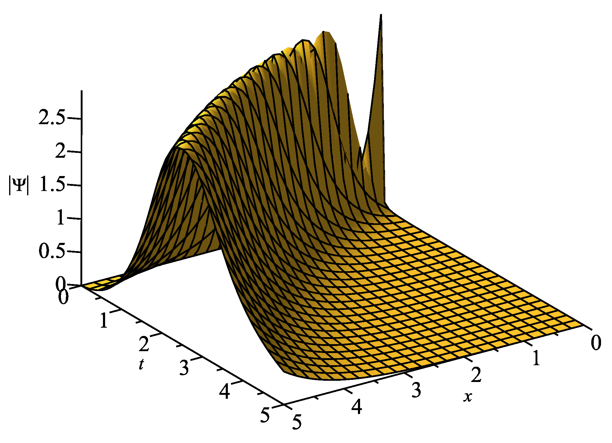
7. Interpreting Graphical Representations

The dynamics of solitons in the model of the space–time fractional complex GL equation is described graphically. In order to understand the physical properties of the obtained results, some of the derived solutions are depicted by selecting different values of parameters. For example, the 3D plot of solutions (35) and (36) is represented with different values of fractional parameters in Figure 1, where $\alpha =0.3,\beta =0.6$ in Figure 1a and $\alpha =0.5,\beta =0.5$ in Figure 1b. Both soliton solutions (35) and (36) are singular-type solutions with Kerr law nonlinearity. It can be seen that the shape in Figure 1b is symmetric when $\alpha =\beta$. Figure 2 demonstrates the 3D plot of bright and singular soliton solutions (46) and (47) with power-law nonlinearity where the graphs are depicted with fractional parameters (a) $\alpha =0.8,\beta =0.4$ and (b) $\alpha =0.5,\beta =0.5$. In Figure 3, the 3D plot of the first type of bright soliton solution (68) with dual-power law nonlinearity is displayed for $\alpha =0.3,\beta =0.6$. The second type of bright and singular soliton solutions given by (81) and (82) with dual-power law nonlinearity are shown in Figure 4 for the values (a) $\alpha =0.1,\beta =0.1$ and (b) $\alpha =0.8,\beta =0.4$. It is clear that the symmetry of the bright soliton in Figure 4a is due to $\alpha =\beta$.

As we can see, the changes in the parameters cause a clear effect on the dynamics of solitons. In particular, the fractional derivative parameters $\alpha$ and $\beta$ lead to a remarkable variation in the behaviour of the soliton profile.

By comparing the results obtained here with those of previous studies, it is found that the bright and singular optical soliton solutions are different from those obtained in the previous studies. For example, the bright soliton solution (31) with Kerr law effect has a different expression compared to solutions (43) and (47) in [27]. The change in the behaviours of solution (31) in this work and solution (47) in [27] is displayed in Figure 5.

8. Discussion and Conclusions

The present study concentrated on the conformable space–time fractional complex GL equation under the dominance of three different laws of nonlinearity. The types of nonlinear effects are given in the form of the Kerr law, power law, and dual-power law. The model of fractional complex GL equation is reduced to a first-order nonlinear ordinary differential equation (ODE) which is different from the ones derived in all previous studies. Then, a special transformation is used to convert this ODE to a simple equation having a solution expressed in terms of the Weierstrass elliptic function. Applying the relation between the Weierstrass elliptic function and hyperbolic functions, the optical soliton solutions of the conformable space–time fractional complex GL equation are retrieved. The structure of extracted bright and singular optical soliton solutions are different from their corresponding solutions in the previous studies. The type of dark optical soliton is not derived in this study but it can be obtained by applying other integration schemes. The limitations for the validity of solitons are presented. Moreover, the 3D plots of some obtained solitons are illustrated by selecting different values of parameters to show the influence of changing parameter values, especially the fractional derivative parameters, on the soliton behaviour.

References

1. Porsezian, K.; Nakkeeran, K. Optical solitons in presence of Kerr dispersion and self-frequency shift. Phys. Rev. Lett. 1996, 76, 3955. [Google Scholar] [CrossRef]
2. Gedalin, M.; Scott, T.; Band, Y. Optical solitary waves in the higher order nonlinear Schrödinger equation. Phys. Rev. Lett. 1997, 78, 448. [Google Scholar] [CrossRef] [Green Version]
3. Radhakrishnan, R.; Kundu, A.; Lakshmanan, M. Coupled nonlinear Schrödinger equations with cubic-quintic nonlinearity: Integrability and soliton interaction in non-Kerr media. Phys. Rev. E 1999, 60, 3314. [Google Scholar] [CrossRef] [PubMed] [Green Version]
4. Hong, W.P. Optical solitary wave solutions for the higher order nonlinear Schrödinger equation with cubic-quintic non-Kerr terms. Opt. Commun. 2001, 194, 217–223. [Google Scholar] [CrossRef]
5. Biswas, A.; Konar, S. Introduction to non-Kerr Law Optical Solitons; Chapman and Hall/CRC: London, UK, 2006. [Google Scholar]
6. Biswas, A.; Mirzazadeh, M.; Savescu, M.; Milovic, D.; Khan, K.R.; Mahmood, M.F.; Belic, M. Singular solitons in optical metamaterials by ansatz method and simplest equation approach. J. Mod. Opt. 2014, 61, 1550–1555. [Google Scholar] [CrossRef]
7. Zayed, E.; Alurrfi, K. New extended auxiliary equation method and its applications to nonlinear Schrödinger-type equations. Optik 2016, 127, 9131–9151. [Google Scholar] [CrossRef]
8. Arnous, A.H.; Ullah, M.Z.; Moshokoa, S.P.; Zhou, Q.; Triki, H.; Mirzazadeh, M.; Biswas, A. Optical solitons in birefringent fibers with modified simple equation method. Optik 2017, 130, 996–1003. [Google Scholar] [CrossRef]
9. Al-Ghafri, K. Soliton-type solutions for two models in mathematical physics. Waves Random Complex Media 2018, 28, 261–269. [Google Scholar] [CrossRef]
10. Biswas, A.; Ekici, M.; Sonmezoglu, A.; Zhou, Q.; Moshokoa, S.P.; Belic, M. Chirped solitons in optical metamaterials with parabolic law nonlinearity by extended trial function method. Optik 2018, 160, 92–99. [Google Scholar] [CrossRef]
11. Foroutan, M.; Manafian, J.; Ranjbaran, A. Solitons in optical metamaterials with anti-cubic law of nonlinearity by generalized G/G-expansion method. Optik 2018, 162, 86–94. [Google Scholar] [CrossRef]
12. Biswas, A.; Rezazadeh, H.; Mirzazadeh, M.; Eslami, M.; Ekici, M.; Zhou, Q.; Moshokoa, S.P.; Belic, M. Optical soliton perturbation with Fokas–Lenells equation using three exotic and efficient integration schemes. Optik 2018, 165, 288–294. [Google Scholar] [CrossRef]
13. Al-Ghafri, K.S. Solitary wave solutions of two KdV-type equations. Open Phys. 2018, 16, 311–318. [Google Scholar] [CrossRef]
14. Al-Ghafri, K.; Krishnan, E.; Biswas, A.; Ekici, M. Optical solitons having anti-cubic nonlinearity with a couple of exotic integration schemes. Optik 2018, 172, 794–800. [Google Scholar] [CrossRef]
15. Biswas, A.; Arshed, S. Application of semi-inverse variational principle to cubic-quartic optical solitons with kerr and power law nonlinearity. Optik 2018, 172, 847–850. [Google Scholar] [CrossRef]
16. Kader, A.A.; Latif, M.A.; Zhou, Q. Exact optical solitons in metamaterials with anti-cubic law of nonlinearity by Lie group method. Opt. Quantum Electron. 2019, 51, 30. [Google Scholar] [CrossRef]
17. Krishnan, E.; Biswas, A.; Zhou, Q.; Alfiras, M. Optical soliton perturbation with Fokas–Lenells equation by mapping methods. Optik 2019, 178, 104–110. [Google Scholar] [CrossRef]
18. Zayed, E.M.; Alngar, M.E.; Al-Nowehy, A.G. On solving the nonlinear Schrödinger equation with an anti-cubic nonlinearity in presence of Hamiltonian perturbation terms. Optik 2019, 178, 488–508. [Google Scholar] [CrossRef]
19. Al-Ghafri, K. Different Physical Structures of Solutions for a Generalized Resonant Dispersive Nonlinear Schrödinger Equation with Power Law Nonlinearity. J. Appl. Math. 2019, 2019. [Google Scholar] [CrossRef]
20. Al-Ghafri, K.; Rezazadeh, H. Solitons and other solutions of (3 + 1)-dimensional space–time fractional modified KdV–Zakharov–Kuznetsov equation. Appl. Math. Nonlinear Sci. 2019, 4, 289–304. [Google Scholar] [CrossRef] [Green Version]
21. Oliveira, D.S.; de Oliveira, E.C. On a Caputo-type fractional derivative. Adv. Pure Appl. Math. 2019, 10, 81–91. [Google Scholar] [CrossRef]
22. Atanacković, T.M.; Pilipović, S.; Zorica, D. Properties of the Caputo-Fabrizio fractional derivative and its distributional settings. Fract. Calc. Appl. Anal. 2018, 21, 29–44. [Google Scholar] [CrossRef] [Green Version]
23. Ortigueira, M.D. Fractional Calculus for Scientists and Engineers; Springer Science & Business Media: Berlin, Germany, 2011; Volume 84. [Google Scholar]
24. Jacobs, B.A. A new Grünwald-Letnikov derivative derived from a second-order scheme. Abstr. Appl. Anal. 2015, 2015, 952057. [Google Scholar] [CrossRef] [Green Version]
25. Khalil, R.; Al Horani, M.; Yousef, A.; Sababheh, M. A new definition of fractional derivative. J. Comput. Appl. Math. 2014, 264, 65–70. [Google Scholar] [CrossRef]
26. Tasbozan, O.; Kurt, A.; Tozar, A. New optical solutions of complex Ginzburg–Landau equation arising in semiconductor lasers. Appl. Phys. B 2019, 125, 104. [Google Scholar] [CrossRef]
27. Sulaiman, T.A.; Baskonus, H.M.; Bulut, H. Optical solitons and other solutions to the conformable space–time fractional complex Ginzburg–Landau equation under Kerr law nonlinearity. Pramana 2018, 91, 58. [Google Scholar] [CrossRef]
28. Mirzazadeh, M.; Ekici, M.; Sonmezoglu, A.; Eslami, M.; Zhou, Q.; Kara, A.H.; Milovic, D.; Majid, F.B.; Biswas, A.; Belić, M. Optical solitons with complex Ginzburg–Landau equation. Nonlinear Dyn. 2016, 85, 1979–2016. [Google Scholar] [CrossRef]
29. Arnous, A.H.; Seadawy, A.R.; Alqahtani, R.T.; Biswas, A. Optical solitons with complex Ginzburg–Landau equation by modified simple equation method. Optik 2017, 144, 475–480. [Google Scholar] [CrossRef]
30. Inc, M.; Aliyu, A.I.; Yusuf, A.; Baleanu, D. Optical solitons for complex Ginzburg–Landau model in nonlinear optics. Optik 2018, 158, 368–375. [Google Scholar] [CrossRef]
31. Arshed, S. Soliton solutions of fractional complex Ginzburg–Landau equation with Kerr law and non-Kerr law media. Optik 2018, 160, 322–332. [Google Scholar] [CrossRef]
32. Biswas, A.; Yildirim, Y.; Yasar, E.; Triki, H.; Alshomrani, A.S.; Ullah, M.Z.; Zhou, Q.; Moshokoa, S.P.; Belic, M. Optical soliton perturbation with complex Ginzburg–Landau equation using trial solution approach. Optik 2018, 160, 44–60. [Google Scholar] [CrossRef]
33. Rezazadeh, H. New solitons solutions of the complex Ginzburg-Landau equation with Kerr law nonlinearity. Optik 2018, 167, 218–227. [Google Scholar] [CrossRef]
34. Raza, N. Exact periodic and explicit solutions of the conformable time fractional Ginzburg Landau equation. Opt. Quantum Electron. 2018, 50, 154. [Google Scholar] [CrossRef]
35. Biswas, A. Chirp-free bright optical solitons and conservation laws for complex Ginzburg-Landau equation with three nonlinear forms. Optik 2018, 174, 207–215. [Google Scholar] [CrossRef]
36. Liu, Y.; Chen, S.; Wei, L.; Guan, B. Exact solutions to complex Ginzburg–Landau equation. Pramana 2018, 91, 29. [Google Scholar] [CrossRef]
37. Ahmed, I.; Seadawy, A.R.; Lu, D. Combined multi-waves rational solutions for complex Ginzburg–Landau equation with Kerr law of nonlinearity. Mod. Phys. Lett. A 2019, 34, 1950019. [Google Scholar] [CrossRef]
38. Arshed, S.; Biswas, A.; Mallawi, F.; Belic, M.R. Optical solitons with complex Ginzburg–Landau equation having three nonlinear forms. Phys. Lett. A 2019, 383, 126026. [Google Scholar] [CrossRef]
39. Lawden, D.F. Elliptic Functions and Applications; Springer-Verlag: New York, NY, USA, 1989; Volume 80. [Google Scholar]
40. Chen, Y.; Yan, Z. The Weierstrass elliptic function expansion method and its applications in nonlinear wave equations. Chaos Solitons Fractals 2006, 29, 948–964. [Google Scholar] [CrossRef] [Green Version]
Figure 1. The singular soliton solution (35) with α = 0.3 , β = 0.6 (a) and the singular soliton solution (36) with α = 0.5 , β = 0.5 (b). In both graphs a = ν = γ = 2 , b = c = k = 1 , ω = 4 .
Symmetry 12 00219 g001
Figure 2. The bright soliton solution (46) b = 1 , n = 2 , α = 0.8 , β = 0.4 (a) and the singular soliton solution (47) with b = 1 , n = 1 , α = 0.5 , β = 0.5 (b). In both graphs a = ω = 4 , c = ν = 1 , k = γ = 2 .
Symmetry 12 00219 g002
Figure 3. The bright soliton solution (68) with a = ω = 4 , b 1 = c = ν = 1 , k = n = γ = 2 , α = 0.3 , β = 0.6 .
Symmetry 12 00219 g003
Figure 4. The bright soliton solution (81) with b 2 = 2 , α = 0.1 , β = 0.1 (a) and the singular soliton solution (82) with b 2 = 2 , α = 0.8 , β = 0.4 (b). In both graphs a = ω = 4 , b 1 = c = ν = 1 , k = n = γ = 2 .
Symmetry 12 00219 g004
Figure 5. The bright soliton solutions with a = ω = 4 , b = c = ν = 1 , k = 1 8 , γ = 2 , α = 0.8 , β = 0.5 . (a) Solution (31) in this work and (b) solution (47) in [27].
Symmetry 12 00219 g005