Extraction of Frictional Vibration Features with Multifractal Detrended Fluctuation Analysis and Friction State Recognition

Abstract

For the purpose of extracting the frictional vibration characteristics of the friction pair during friction and wear in different friction states, the friction and wear tests of friction pair in different friction states were conducted on a testing machine. Higher-dimensional fractal and multifractal characteristics hidden in time series can be examined by multifractal detrended fluctuation analysis (MFDFA) method. The frictional vibration time-domain signals, the friction coefficient signals and the frictional vibration frequency-domain signals were analyzed and multifractal spectra were acquired by using the MFDFA algorithm. According to the spectra, the multifractal spectrum parameters of these signals were calculated to realize the quantitative characterization of frictional vibration characteristics in different friction states. The analysis shows that it is symmetric in the variation trends of the multifractal spectrum parameters of the frictional vibration signals and the friction coefficient data. Based on the multifractal spectrum parameters of frictional vibration, the principal component analysis (PCA) algorithm was applied to establish the friction state recognition method. The results show that the multifractal spectra and their parameters can characterize the frictional vibrations, and the friction state recognition can be realized based on the multifractal spectrum parameters of frictional vibrations.

1. Introduction

Frictional vibration is a phenomenon caused by the friction and wear procedure of the friction pair during the operations of mechanical equipment, which contain information reflecting the characters and behaviors of the tribological system. The vibration caused by friction is one of the important tribological information of the friction pairs. The information of tribological system also include the friction coefficient [1,2], the friction torque [3], the surface morphology of the friction pair [4], the condition of the lubricating medium and the wear particles [5]. These are inconvenient methods to extract the tribological characteristics by friction coefficient or friction torque, which is difficult to measure under the condition of equipment operation. In addition, the wear surface topography and wear particle are time-consuming methods, and the accuracy of the analysis results is closely related to the analyst’s experience. [6]. By contrast, the frictional vibration signals can be collected in real time during normal operation of the devices using acceleration sensors. Therefore, some scholars indicated that frictional vibration signals could be applied to recognition of the friction and wear states of the friction pair [7]. Therefore, the analysis of frictional vibrations is a better means to monitor the friction and wear states of the friction pair in real time during the operation of equipment.

The study of the frictional vibration has attracted many scholars’ interest. Jaeyong et al. studied the nonlinear behaviors of the frictional vibration by using spring-mass model based on the smooth friction velocity curve. The results show that the nonlinearity and instability of friction may bring forth chaotic frictional vibrations according to the friction curve [8]. Liu et al. showed that the cross correlation coefficient of frictional vibration is opposite to the variations of friction coefficient [9]. Sun D. et al. pointed out that the change law of the defined frictional vibration parameter k is consistent with the change trends of the friction coefficient during the tests [10]. Rouzic et al. studied the squeal noises of a wiper/windscreen contacts. Based on Stebeck’s law of friction coefficient, they proved that noises are caused by self-excited frictional vibration [11]. Wernitz and Hoffmann’s analysis indicated that irregular frictional vibration states of friction brakes are mainly dominated by intermittency phenomena [12]. Nadim et al. pointed out that the frictional vibration of dry friction has nonlinear characteristics, and the surface morphology of the friction pair change due to abrasive wear and adhesive wear at the interface of the friction pair results in the change of friction coefficient, which is the source of the nonlinear frictional vibration [13]. Recently, scholars have applied some nonlinear physical methods [14], such as the chaos and fractal methods [15,16], to the features extraction of frictional vibrations. Some scholars investigated the attractors of frictional vibration by applying the chaos theory, and they discovered that the chaotic attractors of frictional vibration gradually converge and present some regular changes in the running-in process [17]. Zhu et al. analyzed the fractal dimensions of frictional vibration [18], and they indicated that it is feasible to identify the running-in states by using the fractal dimensions of frictional vibrations.

The multifractal detrended fluctuation analysis (MFDFA) algorithm has been proven to be an effective tool for revealing the multifractality properties of non-stationary time series in various complex systems. At present, MFDFA has been successfully applied to analyzing diverse time-series data, such as three-dimensional surface topography data [19], temperature reanalysis data [20], wind speed records [21], financial data [22], traffic data [23], feature extraction [24], geophysical time series [25], ECG patterns [26], vibration data [27], etc. In this paper, the nonlinear characteristics of frictional vibrations were analyzed by using the MFDFA algorithm to derive the multifractal spectra as well as their parameters. The analysis shows that it is symmetric in the variation trends of the multifractal spectrum parameters of frictional vibrations and friction coefficients. Based on these multifractal spectrum parameters, three friction states—mixed lubrication, boundary lubrication and dry friction of tribological pair—in this experiment were distinguished with principal component analysis (PCA) algorithm. The results show that the frictional vibration signals could be characterized by the MFDFA spectra and their parameters. The research results can provide the theoretical basis and method for the real-time monitoring and fault diagnosis of mechanical equipment.

2. Experiments

2.1. Tribological Pair

A pin-block specimen was used as tribological pair in this experiment. The pin specimen was 6 mm diameter with hardness of 256 HV and surface roughness Sa = 1.031 μm. The material of the pin specimen was gray cast iron and its main ingredients were iron, carbon, silicon, manganese, sulfur, phosphorus, etc. The block specimen was obtained by cutting the cylinder jacket of the marine diesel engine. The block specimen was of cuboid size 43.2 mm × 30.5 mm × 3.2 mm with hardness of 339 HV and surface roughness Sa = 4.749 μm, and its main ingredients were iron, carbon, silicon, manganese, phosphorus, etc.

2.2. Apparatus

The experiments of friction and wear of the pin-block specimen were conducted on a multi-specimen testing machine of UMT-TriboLab type as shown in Figure 1. The major components of the testing machine consist of a driving motor, an acceleration sensor, a force sensor, a signal collecting device as well as a computer system. The pin specimen was contacted vertically against the block specimen with a special jig. A bench, which is driven by an eccentric mechanism, was designed for fixing the block specimen. The electric motor drives the eccentric mechanism which converts the rotation motions into the reciprocating motions. The testing load was 50 N, the horizontal sliding distance of the friction pair was 8 mm and the reciprocating slip frequency was 0.5 Hz. In the test, frictional vibration was measured by means of an acceleration sensor (model PCB-356A16) of PCB PIEZOTRONICS company whose measuring range is ±50 g and sensitivity is 100 mV/g. The frictional vibration data was collected using Vibpilot data acquisition system of m + p international company with the sampling points of 4096 and sampling frequency of 15,360 Hz. The frictional vibration data was subjected to denoising using spectral subtraction [28] and ensemble empirical mode decomposition algorithm [29] for subsequent analysis. The friction coefficient data calculated and stored by the computer of the testing machine are 100 data points per second. These data were saved into the workstation computer system. The surface topography of the friction pair was scanned by using ContourGT optical microscope of the Bruker company, and the surface topography parameters were calculated by the supporting computer.

2.3. Methods

All tests were carried out in an ambient condition with relative humidity from 45 to 60% and temperature from 23 to 27 °C. Friction states of friction pair during tests were: mixed lubrication, boundary lubrication and dry friction. Considering the effects of lubricating oil on the tests, the test times of the three lubrication states tests are different. The Castrol 5W-40 synthetic lubricating oil was used in the tests with density of 0.8588 g/cm³ and viscosity of 80.247 mm²/s at 40 °C. The UMT-TriboLab friction and wear testing machine displayed and recorded the friction coefficient data, and the friction states of the friction pair were determined by controlling the amounts of lubricant and the friction coefficient. Reference [30] gives the typical friction coefficient values of different friction states, e.g., the friction coefficient of mixed lubrication is about 0.01~0.12, the friction coefficient of boundary lubrication is about 0.12~0.3 and the friction coefficient of dry friction is more than 0.3. During the mixed lubrication test, the block sample was fixed in the oil tank and immersed in the lubricating oil completely. The mixed lubrication test was carried out for 60 min. After the completion of the mixed lubrication test, the lubricating oil was completely removed, and the friction surface of the block sample and the pin sample were cleaned by non-woven paper with very thin oil film left. The friction state of the boundary lubrication was determined by the friction coefficient and the boundary lubrication test was carried out for 4 min. After completing boundary lubrication test, the surface of the friction pair was thoroughly cleaned by gasoline and the subsequent dry friction test was carried out for 20 min. The friction coefficient data of the three friction state tests of the mixed lubrication, boundary lubrication and dry friction tested in this paper are shown in Figure 2.

3. MFDFA Algorithm

Detrended fluctuation analysis (DFA) was first introduced by Peng et al. in 1995, is a reliable method for examining the long-range correlations of DNA sequences [31]. Afterwards, an extension of DFA called multifractal detrended fluctuation analysis (MFDFA) was introduced by Kantelhardt et al. in 2002, for detecting the multifractality of non-stationary time series [32]. It has proven to be an effective tool for uncovering the multifractality of such signals. Suppose that the time series x_k of length N is the signal to be analyzed. The MFDFA algorithm includes the following six steps [33]:

Step 1: Determine the “profile”:

$$Y(i)={\displaystyle \sum _{k=1}^i(x_k-\overline{x})}, (i=1,2,\dots ,N)$$

(1)

Step 2: Divide the profile Y(i) into N_s = int(N/s) nonoverlapping segments of equal length s.

Step 3: The local trend for each of the 2N_s segments is calculated by a least-square fit of the series. Then determine the variance:

$$F^2(s,v)=\frac{1}{s}{\displaystyle \sum _{i=1}^s{\{Y[v-1]s+i-y_v(i)\}}^2}$$

(2)

For each segment v, v = 1, 2, …, N_s and

$$F^2(s,v)=\frac{1}{s}{\displaystyle \sum _{i=1}^s{\{Y[N-(v-N_s)s+i]-y_v(i)\}}^2}$$

(3)

For v = N_s + 1, N_s + 2, …, 2N_s. In this expression, y_v(i) is the fitting polynomial in segment v.

Step 4: In order to obtain the qth order fluctuation function, Average all segments:

$$F(q,s)={\left\{\frac{1}{2N_s}{\displaystyle \sum _{v=1}^{2N_s}{[F^2(s,v)]}^{q/2}}\right\}}^{1/q}$$

(4)

Step 5: Determine the scaling behavior of the fluctuation functions by analyzing log-log plots F_q(s) versus s for each value of q:

$$F(q,s)~s^{h(q)}$$

(5)

In general, the exponent h(q) may depend on q. When q = 2, The h(2) is identical to the well-known Hurst exponent [34].

Step 6: Determine the singularity spectrum to characterize a multifractal time series, that is related to τ(q) via a Legendre transform [35], τ(q) is the multifractal scaling exponent:

$$\tau (q)=qh(q)-1$$

(6)

$$\mathrm{and} \alpha ={\tau }^{\prime }(q)$$

(7)

then obtain:

$$f(\alpha )=q\alpha -\tau (q)$$

(8)

Here, α is the singularity strength, while f(α) illustrates the dimension of the subset of the time series that is characterized by α. The multifractal spectrum gives numerous information about the variation in the fractal structure of the time series.

4. Applying MFDFA to Signals

The MFDFA algorithm was applied to the feature extraction of the frictional vibration signals and friction coefficient data. For the frictional vibration data of the mixed lubrication friction test, the frictional vibration signals of one complete reciprocating stroke were selected at the times of 1st min, 5th min, 10th min, 20th min, 30th min, 40th min, 50th min, and 60th min, respectively, as the sampling times marked from a to h. The time-domain waveforms and frequency spectra of the frictional vibrations with mixed lubrication are shown in Figure 3. For the frictional vibration data of the boundary lubrication friction test, the frictional vibration signals of one complete reciprocating stroke were selected at the times of 30th sec, 60th sec, 90th sec, 120th sec, 150th sec, 180th sec, 210th sec, and 240th sec, respectively, as the sampling times marked from a to h. Due to space limitations, Figure 4 only shows a typical time-domain waveform and frequency spectrum of the frictional vibrations with boundary lubrication. For the frictional vibration data of the dry friction test, the frictional vibration signals of one complete reciprocating stroke were selected at the times of 1st min, 3rd min, 5th min, 7th min, 10th min, 13th min, 17th min, and 20th min, respectively, as the sampling times marked from a to h. Figure 5 shows a typical time-domain waveform and frequency spectrum of frictional vibrations with dry friction.

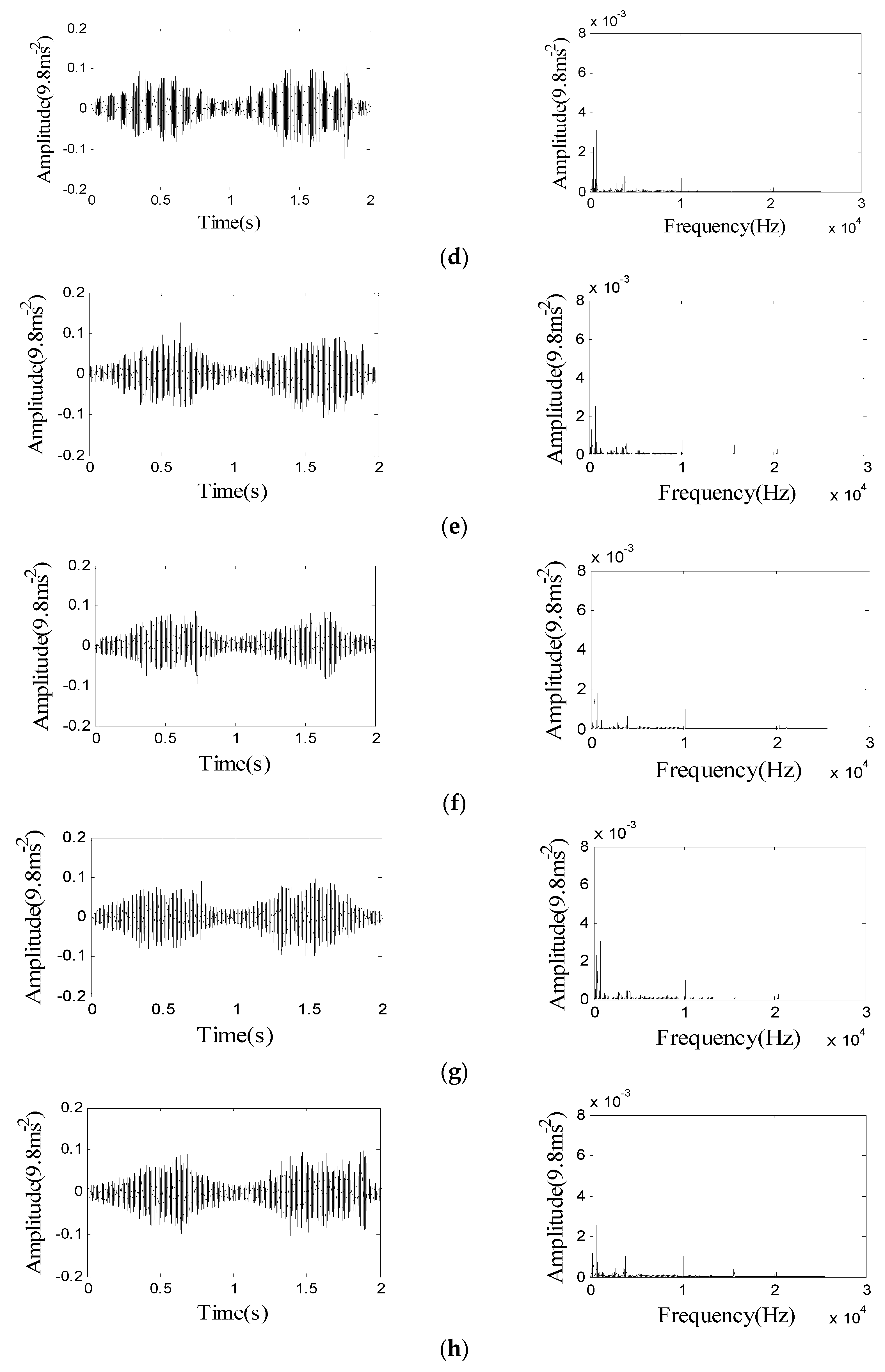
4.1. Applying MFDFA to Frictional Vibration Time-Domain Signals

For the purpose of extracting and quantitatively characterizing the characteristics of the frictional vibrations, the MFDFA was used to the analysis of the frictional vibration signals. Taking the time-domain signal of the frictional vibration shown in Figure 3a as an example, the input parameter q is set as 101 points between −5 and 5, and the segment sample size is set 19 values between 16 and 1024. The qth order weights the influence of segments with large and small fluctuations, as illustrated in Figure 6a, the qth order fluctuation function for negative q’s (i.e., q = −1, −3) are influenced by segments with small root mean squares (RMS). In contrast, the qth order fluctuation function for positive q’s (i.e., q = 1, 3) are influenced by segments with large RMS. The magnitude of the negative or positive qth order grade the local fluctuations with large and small magnitudes, respectively. The qth order fluctuation function for q = −3 and q = 3 is more affected by the segments with the smallest and largest, respectively, compared with qth order fluctuation functions for q = −1 and q =1. The overall q-order measurement units are able to describe the structures of small and large fluctuation of the frictional vibration time series.

The slope of the regression lines in Figure 6a is called the q-order Hurst exponent. The q-order Hurst exponent is a scaling exponent used to parameterize the multifractal structure of times series. As shown in Figure 6b, the q-order Hurst exponents of the frictional vibration signal are greater than 0.5, indicating that the frictional vibration signal has a time-independent structure. The q-order Hurst exponent represents the average fractal structure of the times series, is closely related to the tendency of a multifractal spectrum. The q-order Hurst exponent is transformed to the q-order mass exponent in Equation (6). As shown in Figure 6c, thereafter convert the q-order mass exponent to the q-order singularity exponent in Equation (7) and the q-order singularity dimension in Equation (8). As shown in Figure 6d, the multifractal spectrum is obtained by taking the q-order singularity exponent as the abscissa and the q-order singularity dimension as the ordinate, and the large arc is the resulting multifractal spectrum of the frictional vibration signal. The different scale invariant structures of the frictional vibration signal are classified by the width and shape of the multifractal spectrum. The difference between the maximum and minimum of the multifractal spectrum is called the multifractal spectrum width Δα, and the deviation from average fractal structure for segments with large and small fluctuations is represented by the multifractal spectrum width [33]. The multifractal spectrum dimension difference Δf = f(α_min) − f(α_max), describes how much the number of subset elements formed by a fractal object changes as the segmentation length decreasing. The maximum f_max represents the dominant value in quantity of the signal distributions. The multifractal spectrum critical value α_fmax shows the signal distributions dominant in quantity. The spectrum parameter α_max indicates the minimum value of the signal distributions. The spectrum parameter I_α = α_fmax − α_min represents the numerical difference between the signal distribution dominant in quantity and maximum value, manifesting the uniformity of the signal.

The multifractal spectra of the time-domain signals with the frictional vibrations in different friction states are shown in Figure 7. The curves of the multifractal spectra determined by the frictional vibration signals are constantly changing in shapes with the progress of the test time. The shapes of the curves in different friction states are similar with different parameter ranges. It is shown that the frictional vibration signals obtained by the friction and wear tests of the friction pair have multifractal characteristics, and these multifractal spectra reflect certain regularities. As shown in Figure 8, the spectrum parameters Δα, Δf, f_max, α_fmax, α_max, and I_α were calculated based on the multifractal spectra of the time-domain signals of the frictional vibrations.

As shown in Figure 8, during the mixed lubrication test, the multifractal spectrum parameters of the frictional vibration time-domain signals show certain trends. The multifractal spectrum width Δα exhibits tendency of decreasing with ranges between 1.28 and 0.95. The difference in the number of large and small amplitudes of frictional vibrations present decreasing trend, and the parameter Δf shows decreasing trends with ranges between 0.60 and 0.30. The dominant value in the number of amplitudes decreases, and the f_max also shows decreasing trends with ranges between 1.01 and 0.93. The multifractal spectrum critical value of frictional vibrations decreases, and the α_fmax illustrates decreasing trends with ranges between 0.85 and 0.53. The multifractal spectrum parameter α_max indicates decreasing trends with ranges between 1.92 and 1.31. Frictional vibrations tend to be uniform, and I_α demonstrates decreasing trends with ranges between 0.20 and 0.17.

During the boundary lubrication test, the multifractal spectrum width Δα exhibits tendency of increasing with ranges between 1.23 and 1.52. The multifractal spectrum parameter Δf shows increasing trends with ranges between 0.34 and 0.59. The f_max also shows increasing trends with ranges between 0.93 and 0.95. The α_fmax illustrates increasing trends with ranges between 0.68 and 0.70. The α_max indicates increasing trends with ranges between 1.61 and 1.94. The multifractal spectrum parameter I_α demonstrates increasing trends with ranges between 0.23 and 0.28.

During the dry friction test, the multifractal spectrum width Δα exhibits tendency of increasing with ranges between 1.26 and 1.54. The multifractal spectrum parameter Δf shows increasing trends with ranges between 0.20 and 0.43. The f_max also shows increasing trends with ranges between 0.94 and 0.98. The α_fmax illustrates increasing trends with ranges between 0.59 and 0.73. The α_max indicates increasing trends with ranges between 1.56 and 1.84. The multifractal spectrum parameter I_α demonstrates increasing trends with ranges between 0.29 and 0.43.

4.2. Applying MFDFA to Friction Coefficient Data

The frictional coefficient data of different friction state tests shown in Figure 2 was analyzed by using MFDFA algorithm. For the frictional coefficient data of the mixed lubrication friction test, the frictional coefficient data with 30 s was selected at the times of 1st min, 5th min, 10th min, 20th min, 30th min, 40th min, 50th min, and 60th min, respectively, as the sampling times marked from a to h. For the frictional coefficient data of the boundary lubrication friction test, the frictional coefficient data were selected at the times of 0~30 s, 30~60 s, 60~90 s, 90~120 s, 120~150 s, 150~180 s, 180~210 s, and 210~240 s, respectively, as the sampling times marked from a to h. For the frictional coefficient data of the dry friction test, the frictional coefficient data with 30 s were selected at the times of 1st min, 3rd min, 5th min, 7th min, 10th min, 13th min, 17th min, and 20th min, respectively, as the sampling times marked from a to h. The friction coefficient data calculated and stored by the computer of the testing machine are 100 data points per second, and each of the above stages contains 3000 data points. The multifractal spectra obtained by the analysis of the friction coefficient data are shown in Figure 9 and Figure 10 is the spectrum parameters Δα, Δf, f_max, α_fmax, α_max, and I_α calculated based on the multifractal spectra.

As shown in Figure 10, during the mixed lubrication test, the multifractal spectrum parameters of the friction coefficient data show certain trends. The multifractal spectrum width Δα exhibits tendency of decreasing with ranges between 0.211 and 0.160. The difference in the number of large and small amplitudes of the friction coefficient data present decreasing trend, and the parameter Δf shows decreasing trends with ranges between 0.352 and 0.296. The dominant value in the number of the friction coefficient data reduce, and the f_max also shows decreasing trends with ranges between 1.0231 and 1.0228. The multifractal spectrum critical value of the friction coefficient data decrease, and the α_fmax illustrates decreasing trends with ranges between 1.027 and 1.023. The multifractal spectrum parameter α_max indicates decreasing trends with ranges between 1.186 and 1.154. The multifractal spectrum parameter I_α demonstrates decreasing trends with ranges between 0.053 and 0.028.

During the boundary lubrication test, the multifractal spectrum width Δα exhibits tendency of increasing with ranges between 0.158 and 0.175. The multifractal spectrum parameter Δf shows increasing trends with ranges between 0.289 and 0.452. The f_max also shows increasing trends with ranges between 1.0229 and 1.0231. The α_fmax illustrates increasing trends with ranges between 1.0257 and 1.0264. The α_max indicates increasing trends with ranges between 1.152 and 1.177. The multifractal spectrum parameter I_α demonstrates increasing trends with ranges between 0.025 and 0.027.

During the dry friction test, the multifractal spectrum width Δα exhibits tendency of increasing with ranges between 0.197 and 1.208. The multifractal spectrum parameter Δf shows increasing trends with ranges between 0.361 and 0.462. The f_max also shows increasing trends with ranges between 1.0230 and 1.0232. The α_fmax illustrates increasing trends with ranges between 1.0265 and 1.0269. The α_max indicates increasing trends with ranges between 1.205 and 1.216. The multifractal spectrum parameter I_α demonstrates increasing trends with ranges between 0.018 and 0.022.

4.3. Applying MFDFA to Frictional Vibration Frequency-Domain Signals

The frequency-domain signals of the frictional vibrations, obtained by Fourier transform of the frictional vibration time-domain signals in Figure 3, also contain important information. The frequency-domain signals of the frictional vibrations are analyzed by the MFDFA algorithm, and the multifractal spectra obtained are shown in Figure 11 and Figure 12 is the spectrum parameters Δα, Δf, f_max, α_fmax, α_max, and I_α calculated based on the multifractal spectra.

As shown in Figure 12, during the mixed lubrication test, the multifractal spectrum parameters of the frictional vibration frequency-domain signals show certain trends. The multifractal spectrum width Δα exhibits tendency of decreasing with ranges between 1.21 and 0.98. The parameter Δf shows decreasing trends with ranges between −0.02 and −0.47. The dominant value in the number of the frictional vibration frequency-domain signals reduce, and the f_max also shows decreasing trends with ranges between 1.0172 and 1.0168. The multifractal spectrum critical value α_fmax illustrates decreasing trends with ranges between 1.084 and 1.072. The multifractal parameter α_max indicates decreasing trends with ranges between 1.82 and 1.51. Frictional vibrations tend to be uniform, and I_α demonstrates decreasing trends with ranges between 0.47 and 0.53.

During the boundary lubrication test, the multifractal spectrum width Δα exhibits tendency of increasing with ranges between 0.99 and 1.11. The multifractal spectrum parameter Δf shows increasing trends with ranges between −0.50 and −0.35. The f_max also shows increasing trends with ranges between 1.0170 and 1.0174. The α_fmax illustrates increasing trends with ranges between 1.07 and 1.11. The α_max indicates increasing trends with ranges between 1.50 and 1.62. The multifractal spectrum parameter I_α demonstrates increasing trends with ranges between 0.56 and 0.61.

During the dry friction test, the multifractal spectrum width Δα exhibits tendency of increasing with ranges between 0.94 and 1.24. The multifractal spectrum parameter Δf shows increasing trends with ranges between −0.43 and −0.24. The f_max also shows increasing trends with ranges between 1.0171 and 1.0174. The α_fmax illustrates increasing trends with ranges between 1.08 and 1.11. The α_max indicates increasing trends with ranges between 1.54 and 1.68. The I_α demonstrates increasing trends with ranges between 0.48 and 0.67.

As shown in Figure 8, Figure 10 and Figure 12, some multifractal spectrum parameters are fluctuated with non-monotonical variation tendency because the microscopic path of each reciprocating motion of friction pair is not repeated in the test processes, but the increasing or decreasing trends of the multifractal spectrum parameters can be used as the basis for analysis.

4.4. Analysis and Discussions

Figure 13 is the surface topographies of the block specimen at different test moments.

Table 1. The surface topography parameters of the block specimen.

Parameters	Block Specimen Initial	End of Mixed Lubrication	End of Boundary Lubrication	End of Dry Friction
Sa (μm)	4.749	3.185	2.524	2.787
Ssk	−0.693	−0.51	−1.376	−1.833
Sz (μm)	63.785	54.635	36.367	37.756

is the surface topography parameters of the block specimen. The S_a is the mean roughness, and S_a can be used to indicate significant deviations in the texture. The S_sk is the skewness of the surface texture representing the degree of symmetry of the surface heights about the mean plane, the S_sk shows the preponderance of peaks (that is, S_sk > 0) or valley structures (S_sk < 0) comprising the surface. The S_z is the ten points height over the surface, and the S_z characterizes the maximum peak to valley magnitude for the entire surface [36].

As shown in Figure 13a and Table 1, prior to the test, the initial roughness of the block specimen surface is large with many micro-convex peaks on the surface topography. The surface heights of the block specimen fluctuate in a large range. At the beginning of the mixing lubrication test, the amplitudes of the frictional vibrations are uneven, and the fluctuation amplitude range is large. Thus, the spectrum parameters Δα, Δf, f_max, α_fmax, α_max, and I_α of the frictional vibrations are large. As the mixed lubrication test proceeds, many micro-convex peaks of different shapes on the surface of the friction pair are continuously flattened. Figure 13b shows the surface topography of the block specimen at the end of mixed lubrication test, and the surface roughness reduces obviously. Besides, the parameter S_sk is negative with shrinking value, indicating the preponderance of valley structures decreases. The S_z value decreases, indicating the maximum peak to valley magnitude decreases. Thus, the frictional vibrations excited tend to be stabilized with the roughness reduced and the relative contact area increased. The spectrum parameters Δα, Δf, f_max, α_fmax, α_max, and I_α of the frictional vibrations show decreasing trends. During the boundary lubrication test, there is very thin oil film existing in the surface of the friction pair, and there are more micro-convex peaks contact. As shown in Figure 13c, the surface roughness reduces and the surface topography consists of a number of small contact plateaus. The frictional vibration is violent and its amplitude is high. Thus, the spectrum parameters Δα, Δf, f_max, α_fmax, α_max, and I_α of the frictional vibrations show increasing trends. During the dry fraction test, the lubrication condition is so bad that the micro-convex peaks are contact directly. Besides, the surface roughness of friction pair increases, the S_sk is negative with growing value, indicating the preponderance of valley structures increases. The S_z value increases, indicating the maximum peak to valley magnitude increases. Figure 13d shows the surface topography of the block specimen at the end of dry friction test. The surface is severely damaged due to the generation of many deep furrows, and the surface heights fluctuate violently in a large range. The frictional vibrations excited are severe. Thus, the spectrum parameters Δα, Δf, f_max, α_fmax, α_max, and I_α of the frictional vibrations show increasing trends.

For friction coefficient data of the tests, during the mixed lubrication test, the high peaks on the block specimen are worn off gradually with the surface roughness decreasing, and the friction forces decrease with good lubrication condition. The friction coefficients show downward trends with the friction forces decreasing. Thus, the spectrum parameters Δα, Δf, f_max, α_fmax, α_max, and I_α of the friction coefficient show decreasing trends. During the boundary lubrication test, there is very thin oil film existing in the surface of the friction pair, and the friction forces increase with more micro-convex peaks contact. The friction coefficients display upward trends. Thus, the spectrum parameters Δα, Δf, f_max, α_fmax, α_max, and I_α of the friction coefficient data show increasing trends. During the dry fraction test, the lubrication condition is so bad that the micro-convex peaks are contact directly. The friction coefficients show upward trends with the friction forces increasing. Thus, the spectrum parameters Δα, Δf, f_max, α_fmax, α_max, and I_α of the friction coefficient data show increasing trends.

It can be seen from Figure 8 and Figure 10 that the variation trends of the multifractal spectrum parameters of the frictional vibration time-domain signals consist with the variation trends of the multifractal spectrum parameters of the friction coefficient data within the same lubrications, indicating the symmetry of the fractal structures of the two signals. The friction coefficients can directly reflect the friction states of the friction pair. So the frictional vibrations can be used for the recognitions of the friction states based on the multifractal spectrum parameters.

5. Friction State Recognition

5.1. Principal Component Analysis Algorithm

PCA algorithm transforms an original data with correlated variables into a smaller set of new variables, and the new variables are uncorrelated and retains most information of the original data [37]. Supposed that the original data matrix with n samples and m variables can be given by:

$$X_0={[x_1,x_2,\dots ,x_n]}^T=\left[\begin{array}{ccc}{x}_{1,1}& \dots & x_{1,m}\\ .& \dots & .\\ x_{n,1}& \dots & x_{n,m}\end{array}\right]$$

(9)

X₀ is normalized first by the following equation to eliminate the influences of variable dimension and sample quantity in the original data:

$$x_{i,j,0}=\frac{x_{i,j}-{\overline{x}}_j}{\sigma }=\frac{x_{i,j}-\frac{1}{n}{\displaystyle {\sum }_{i=1}^n{x}_{i,j}}}{\sqrt{\frac{1}{n}{\displaystyle {\sum }_{i=1}^n{(x_{i,j}-\frac{1}{n}{\displaystyle {\sum }_{i=1}^n{x}_{i,j}})}^2}}}$$

(10)

X can be given by:

$$X=\left[\begin{array}{ccc}{x}_{1,1,0}& \dots & x_{1,m,0}\\ .& \dots & .\\ x_{n,1,0}& \dots & x_{n,m,0}\end{array}\right]$$

(11)

And then X is projected onto a new space ordinate system by the following linear transformation:

$$T=[t_1,t_1,\dots ,t_m]=XP=X[p_1,p_2,\dots ,p_m]$$

(12)

where T is the score matrix, and the vectors t_i in T are orthonormal. These orthonormal vectors are the linear combination of X that show how samples are related to each other. P is the loading matrix which is derived from the covariance matrix of X. Vectors p_i in P are orthonormal, and they are the dimensions in the new orthonormal coordinate system. P can be derived from the following eigenvalue problem:

$$C=P\Lambda P^T$$

(13)

where C is the covariance matrix of X, and $\Lambda =diag({\lambda }_1,{\lambda }_2,\dots ,{\lambda }_m)$. Additionally, ${\mathsf{\lambda }}_i$ exhibit the variation contained on the dimension of p_i in the new space.

Then the principal components (PCs) in the new space can be determined according to the distribution of variation in the new coordinate system. There are different criteria to determine the number of PCs in a PCA model [38]. In this paper, the cumulative percent variance (CPV) criterion is adopted, since the eigenvalues describe how much information each PC contains. The CPV represents the variation of the selected k PCs account for all the variation in X:

$$CPV=\frac{{\displaystyle {\sum }_{i=1}^{i=k}{\lambda }_i}}{{\displaystyle {\sum }_{i=1}^{i=m}{\lambda }_i}}\times 100\%$$

(14)

The greater the cumulative percent variance, the stronger the information that the principal component contains the original variables. The number of principal components k is selected according to the cumulative percent variance of the principal components. Generally, the cumulative percent variance is required to be greater than 85% to ensure that the comprehensive variables can include most of the information of the original variables [39,40].

5.2. Analysis and Discussions

In order to identify the friction states of the friction pair through the frictional vibration signals, principal component analysis algorithm is applied to analyzing the multifractal spectrum parameters of the frictional vibration time-domain signals and the frequency-domain signals in friction and wear tests of three friction states: mixed lubrication, boundary lubrication and dry friction. The multifractal spectrum parameters ∆α, ∆f, f_max, ${\alpha }_{f_{\max }}$, α_max, I_α of the frictional vibration time-domain signals and the frequency-domain signals are shown in Figure 8 and Figure 12. The 12 variables consist of six time-domain multifractal spectrum parameters and six frequency-domain multifractal spectrum parameters. Each of the eight frictional vibration signals selected from the states of mixed lubrication, boundary lubrication and dry frication, respectively, constitute the data matrix of 24 samples and 12 variables. By analyzing results, the first three principal component eigenvalues and percent variance are shown in

Table 2. The first three principal component eigenvalues and percent variance.

Principal Component	Eigenvalues	Percent Variance%
The first	5.8786	48.9889
The second	3.4176	28.4801
The third	1.7415	14.5121

. The CPVs of the first three principal components are shown in

Table 3. The Cumulative Percent Variance (CPV) of the first three principal components.

Principal Component	Cumulative Percent Variance (CPV)%
The first	48.9889
The first + the second	77.4690
The first + the second + the third	91.9811

. The CPV of the first three principal components is 91.9811%, indicating that the first three principal components contain most of the characteristic information.

The first three principal components are obtained as shown in

Table 4. The first three principal components of frictional vibrations in different lubrication states.

Mixed Lubrication			Boundary Lubrication			Dry Friction
The First Principal Component	The Second Principal Component	The Third Principal Component	The First Principal Component	The Second Principal Component	The Third Principal Component	The First Principal Component	The Second Principal Component	The Third Principal Component
−0.7896	2.0636	1.9273	−0.9732	−0.3196	−3.6385	0.9897	−1.3864	1.9019
−1.4366	2.2550	0.3800	−0.7220	−0.0861	−3.1720	1.9564	−0.8116	0.1820
−2.1462	2.9779	1.6202	−0.9069	−1.5494	−1.6859	2.2432	0.8836	−0.3994
−2.0151	3.2316	−0.4073	−0.5071	−2.2932	−0.0743	1.5996	−0.3241	0.5384
−2.0641	0.9125	−0.2715	−0.0323	−1.4850	−0.6901	3.3515	0.7103	−0.0342
−2.7968	0.3663	0.5866	−0.1894	−3.2170	−1.1709	3.3065	2.3175	−1.8440
−2.8594	0.3683	0.7395	0.2357	−2.9844	−0.7245	3.3298	1.5562	0.5675
−2.7226	0.1705	0.0153	−0.5426	−3.2542	0.1757	2.8816	1.5018	0.7907

. The first three columns in Table 4 are the first three principal components corresponding to the mixed lubrication, the middle three columns are the first three principal components corresponding to the boundary lubrication, and the last three columns are the first three principal components corresponding to the dry friction. The first three principal components of Table 4 are mapped to a three-dimensional space, that is, the first principal component, the second principal component, and the third principal component of each signal correspond to one coordinate in the three-dimensional space. Each of the friction states of mixed lubrication, boundary lubrication, and dry friction corresponds to eight coordinates, a total of 24 coordinates. The distribution of these principal components in the three-dimensional space is shown in Figure 14. It can be seen that the characteristic information of the frictional vibration signals in different friction states are distributed in the three-dimensional space.

As shown in Figure 14, the black circles are the first three principal component distribution of the multifractal spectrum parameters of the mixed lubrication frictional vibration signals in three-dimensional space, the red trilaterals the boundary lubrication, and the blue five-pointed stars the dry friction. It can be seen from Figure 14 that the first three components of the frictional vibration multifractal spectrum parameters of the mixed lubrication, boundary lubrication and dry friction have their respective positions in a three-dimensional space. The first three principal components of the same friction states are close to each other with different states in different spatial zones. Three 2-D projection views of Figure 14a are shown in Figure 14b,c,d. The three friction states can be distinguished in Figure 14b,c, but they cannot be distinguished in Figure 14d. It is shown that the principal component analysis based on the multifractal spectrum parameters of frictional vibration can realize the friction state recognition. Meanwhile, the effectiveness of the MFDFA algorithm to extract the frictional vibration characteristics of different friction states is also verified.

For comparison, if the PCA algorithm is used to analyze the frictional vibration time-domain signals directly. The CPV of the first three principal components is 44.5104%, well below 85%. If the first three principal components are still mapped to a three-dimensional space. The spatial distribution of the first three principal components of frictional vibration time-domain signals in different lubrication states is shown in Figure 15. The three friction states cannot be distinguished in Figure 15. Therefore, it is necessary that the frictional vibration signals are analyzed to obtain a small number of parameters as variables of the matrix by using MFDFA algorithm.

6. Conclusions

In this paper, friction and wear experiments of a pin-block were conducted on an UMT-TriboLab testing machine. The MFDFA algorithm was applied to the feature extractions of the frictional vibration signals and friction coefficient data. The multifractal spectrum parameters of the frictional vibrations were analyzed with PCA algorithm. The results of these studies can be used for the real-time monitoring and fault diagnosis of mechanical equipment. The major conclusions are as follows:

(1)

The multifractal detrended fluctuation analysis algorithm can extract the fractal characteristics of the frictional vibration signals effectively. In different friction states, the multifractal spectrum parameters of the frictional vibrations have different parameter ranges and present different trends. The analysis shows that it is symmetric in the variation trends of the multifractal spectrum parameters of the frictional vibrations and the friction coefficients within the same lubrications. The multifractal spectra and their parameters can characterize the nonlinear characteristics of the frictional vibrations.

(2)

The principal component analysis based on the multifractal spectrum parameters of the frictional vibrations can realize the friction state recognition. The first three components of the frictional vibration multifractal spectrum parameters of the mixed lubrication, boundary lubrication and dry friction have their respective positions in a three-dimensional space and close to each other with different states in different spatial zones. The multifractal spectrum parameters of the frictional vibrations can be used to identify the friction states of the friction pair.

References

1. Miler, D.; Hoic, M.; Domitran, Z.; Zezelj, D. Prediction of friction coefficient in dry-lubricated polyoxymethylene spur gear pairs. Mech. Mach. Theory 2019, 138, 205–222. [Google Scholar] [CrossRef]
2. Zhou, C.J.; Hu, B.; Qian, X.L.; Han, X. A novel prediction method for gear friction coefficients based on a computational inverse technique. Tribol. Int. 2018, 127, 200–208. [Google Scholar] [CrossRef]
3. Goncalves, D.; Cousseau, T.; Gama, A.; Gampos, A.V.; Seabra, J.H.O. Friction torque in thrust roller bearings lubricated with greases, their base oils and bleed-oils. Tribol. Int. 2017, 107, 306–319. [Google Scholar] [CrossRef]
4. Zhu, H.; Ge, S.R.; Huang, X. Experimental study on the characterization of worn surface topography with characteristic roughness parameter. Wear 2003, 255, 309–314. [Google Scholar] [CrossRef]
5. Ge, S.R.; Chen, G.X.; Zhang, X.Y. Fractal characterization of wear particle accumulation in the wear process. Wear 2001, 251, 1227–1233. [Google Scholar]
6. Li, J.M.; Wei, H.J.; Mei, L.Q.; Xu, D.Z. Frictional vibration signal analysis using empirical mode decomposition and rescaled range analysis. J. Shanghai Mari. Univ. 2016, 2, 89–93. [Google Scholar]
7. Ge, S.R.; Zhu, H. Complicate Tribological Systems and Quantitative Study Methods of Their Problems. Tribology 2002, 22, 405–408. [Google Scholar]
8. Jaeyoung, K. Lyapunov exponent of friction-induced vibration under smooth friction curve. J. Mech. Sci. Technol. 2018, 32, 3563–3567. [Google Scholar]
9. Liu, T.; Li, G.B.; Wei, H.J.; Sun, D. Experimental observation of cross correlation between tangential friction vibration and normal friction vibration in a running-in process. Tribol. Int. 2016, 97, 77–88. [Google Scholar] [CrossRef]
10. Sun, D.; Li, G.B.; Wei, H.J.; Liao, H.F.; Liu, T. Investigation on frictional vibration behavior of friction pair under different wear state. J. Tribol. Trans. ASME 2015, 137, 021606. [Google Scholar] [CrossRef]
11. Rouzic, J.; Bot, A.; Perret-Liaudet, J. Friction-Induced Vibration by Stribeck’s Law: Application to Wiper Blade Squeal Noise. Tribol. Lett. 2013, 49, 563–572. [Google Scholar] [CrossRef]
12. Wernitz, B.A.; Hoffmann, N.P. Recurrence analysis and phase space reconstruction of irregular vibration in friction brakes. Signatures of chaos in steady sliding. J. Sound Vibr. 2012, 331, 3887–3896. [Google Scholar] [CrossRef]
13. Nadim, A.E.; Hamzeh, T.M.; Montasser, S.T. Stick-slip detection through measurement of near field noise. J. Mech. Eng. Res. 2011, 3, 96–102. [Google Scholar]
14. Zhu, H.; Lu, B.B.; Li, J.Q.; Ji, C.C. Nonlinear theory and methods of researching tribological problems. J. Mech. Eng. 2010, 46, 82–88. [Google Scholar] [CrossRef]
15. Li, G.B.; Huang, Y.H.; Lin, Y.H.; Pan, X.X. Multifractal analysis of frictional vibration in the running-in process. Tribol. Trans. 2013, 56, 284–289. [Google Scholar] [CrossRef]
16. Zhu, H.; Ge, S.R. Chaotic characteristics of tribological systems. Chin. J. Mech. Eng. 2004, 40, 10–13. [Google Scholar] [CrossRef]
17. Sun, D.; Li, G.B.; Wei, H.J. Experimental study on the chaotic attractor evolvement of the friction vibration in a running-in process. Tribol. Int. 2015, 88, 290–297. [Google Scholar] [CrossRef]
18. Zhu, H.; Ge, S.R.; Cao, X.C. The changes of fractal dimensions of frictional signals in the running-in wear process. Wear 2007, 263, 1502–1507. [Google Scholar] [CrossRef]
19. Zuo, X.; Tan, Y.; Zhou, Y.K.; Zhu, H.; Fang, H.F. Multifractal analysis of three-dimensional surface topographies of GCr15 steel and H70 brass during wear process. Measurement 2018, 125, 196–218. [Google Scholar] [CrossRef]
20. Philippopoulos, K.; Kalamaras, N.; Tzanis, C.G.; Deligiorgi, D.; Koutsogiannis, I. Multifractal detrended fluctuation analysis of temperature reanalysis data over Greece. Atmosphere 2019, 10, 336. [Google Scholar] [CrossRef] [Green Version]
21. Laib, M.; Telesca, L.; Kanevski, M. Long-range fluctuations and multifractality in connectivity density time series of a wind speed monitoring network. Chaos 2018, 28, 033108. [Google Scholar] [CrossRef] [PubMed] [Green Version]
22. Gunay, S. Performance of the multifractal model of asset returns (MMAR): Evidence from emerging stock markets. Int. J. Financial Stud. 2016, 4, 11. [Google Scholar] [CrossRef] [Green Version]
23. Shang, P.J.; Lu, Y.B.; Kamae, S. Detecting long-range correlations of traffic time series with multifractal detrended fluctuation analysis. Chaos Solitons Fractals 2008, 36, 82–90. [Google Scholar] [CrossRef]
24. Li, J.M.; Wei, H.J.; Wei, L.D.; Fan, L. Multifractal Detrended Fluctuation Analysis of Frictional Vibration Signals in the Running-in Wear Process. Tribol. Lett. 2017, 65, 50. [Google Scholar] [CrossRef]
25. Subhakar, D.; Chamdrasekhar, E. Reservoir characterization using multifractal detrended fluctuation analysis of geophysical well-log data. Physica A 2016, 445, 57–65. [Google Scholar] [CrossRef]
26. Dutta, S. Multifractal properties of ECG patterns of patients suffering from congestive heart failure. J. Stat. Mech. 2010, 12, 1–14. [Google Scholar] [CrossRef]
27. Vitanov, N.K.; Hoffmann, N.P.; Wernitz, B. Nonlinear time series analysis of vibration data from a friction brake: SSA, PCA, and MFDFA. Chaos Solitons Fractals 2014, 69, 90–99. [Google Scholar] [CrossRef] [Green Version]
28. McMahan, W.; Kuchenbecker, K.J. Spectral subtraction of robot motion noise for improved event detection in tactile acceleration signals. EuroHaptics 2012, 7282, 326–337. [Google Scholar]
29. Chen, R.X.; Tang, B.P.; Ma, J.H. Adaptive de-noising method based on ensemble empirical mode decomposition for vibration signal. J. Vibr. Shock 2012, 31, 82–86. [Google Scholar]
30. Wen, S.Z.; Huang, P.; Tian, Y. Principles of Tribology; Tsinghua University Press: Beijing, China, 2018. [Google Scholar]
31. Peng, C.K.; Buldyrev, S.V.; Havlin, S.; Simons, M.; Goldberger, A.L. Mosaic organization of dna nucleotides. Phys. Rev. E Stat. Phys. Plasmas Fluids Relat. Interdiscip. Top. 1994, 49, 1685–1689. [Google Scholar] [CrossRef] [Green Version]
32. Kantelhardt, J.W.; Zschiegner, S.A.; Koscielny, E. Multifractal detrended fluctuation analysis of nonstationary time series. Physica A 2002, 316, 87–114. [Google Scholar] [CrossRef] [Green Version]
33. Ihlen, E.A.F. Introduction to multifractal detrended fluctuation analysis in Matlab. Front. Physiol. 2012, 141, 1–18. [Google Scholar] [CrossRef] [PubMed] [Green Version]
34. Feder, J. Fractals; Plenum Press: New York, NY, USA, 1988. [Google Scholar]
35. Zia, R.K.P.; Redish, E.F.; McKay, S.R. Making sense of the Legendre transform. Am. J. Phys. 2009, 7, 614–622. [Google Scholar] [CrossRef] [Green Version]
36. Bai, X.Q.; Xie, G.T.; Fan, H.; Peng, Z.X.; Yuan, C.Q.; Yan, X.P. Study on biomimetic preparation of shell surface microstructure for ship antifouling. Wear 2013, 306, 285–295. [Google Scholar] [CrossRef]
37. Li, W.; Peng, M.J.; Wang, Q.Z. False alarm reducing in PCA method for sensor fault detection in a nuclear power plant. Ann. Nucl. Energy 2018, 118, 131–139. [Google Scholar] [CrossRef]
38. Valle, S.; Li, W.H.; Qin, S.J. Selection of the number of principal components: The variance of the reconstruction error criterion with a comparison to other methods. Ind. Eng. Chem. Res. 1999, 38, 4389–4401. [Google Scholar] [CrossRef]
39. Li, G.; Hu, Y. An enhanced PCA-based chiller sensor fault detection method using ensemble empirical mode decomposition based denoising. Energy Build. 2019, 183, 311–324. [Google Scholar] [CrossRef]
40. Zhang, S.; Tang, Q.; Lin, Y.; Tang, Y. Fault detection of feed water treatment process using PCA-WD with parameter optimization. ISA Trans. 2017, 68, 313–326. [Google Scholar] [CrossRef]
Figure 1. UMT-TriboLab friction and wear testing machine. (a) schematic; (b) main components.
Symmetry 12 00272 g001
Figure 2. The friction coefficient data of the three friction state tests. (a) mixed lubrication; (b) boundary lubrication; (c) dry friction.
Symmetry 12 00272 g002
Figure 3. The time-domain waveforms and frequency spectra of frictional vibrations with mixed lubrication. (a) 1st min; (b) 5th min; (c) 10th min; (d) 20th min; (e) 30th min; (f) 40th min; (g) 50th min; (h) 60th min.
Symmetry 12 00272 g003aSymmetry 12 00272 g003b
Figure 4. Typical time-domain waveform and frequency spectrum of frictional vibrations with boundary lubrication.
Symmetry 12 00272 g004
Figure 5. Typical time-domain waveform and frequency spectrum of frictional vibrations with dry friction.
Symmetry 12 00272 g005
Figure 6. Multifractal detrended fluctuation analysis of frictional vibration signal. (a) the qth order fluctuation function; (b) the q-order Hurst exponent; (c) the q-order singularity exponent and singularity dimension; (d) multifractal spectrum.
Symmetry 12 00272 g006aSymmetry 12 00272 g006b
Figure 7. Multifractal spectra of time-domain signals with frictional vibrations in different friction states. (a) mixed lubrication; (b) boundary lubrication; (c) dry friction.
Symmetry 12 00272 g007
Figure 8. Variation law of multifractal spectrum parameters of frictional vibration time-domain signals.
Symmetry 12 00272 g008aSymmetry 12 00272 g008b
Figure 9. Multifractal spectra of friction coefficient data in different friction states. (a) mixed lubrication; (b) boundary lubrication; (c) dry friction
Symmetry 12 00272 g009
Figure 10. Variation law of multifractal spectrum parameters of friction coefficient data.
Symmetry 12 00272 g010
Figure 11. Multifractal spectra of frequency-domain signals with frictional vibrations in different friction states. (a) mixed lubrication; (b) boundary lubrication; (c) dry friction.
Symmetry 12 00272 g011
Figure 12. Variation law of multifractal spectrum parameters of frictional vibration frequency-domain signals.
Symmetry 12 00272 g012
Figure 13. The surface topographies of the block specimen. (a) Block specimen initial; (b) End of mixed lubrication; (c) End of boundary lubrication; (d) End of dry friction
Symmetry 12 00272 g013
Figure 14. Spatial distribution of the first three principal components of frictional vibrations in different lubrication states. (a) Spatial distribution of the first three principal components; (b) 1st to 2nd axis plane; (c) 1st to 3rd axis plane; (d) 2nd to 3rd axis plane.
Symmetry 12 00272 g014
Figure 15. Spatial distribution of the first three principal components of frictional vibration time-domain signals in different lubrication states.
Symmetry 12 00272 g015