Abstract
In this current study, we explore the modified homogeneous cosmological model in the background of LRS Bianchi type-I space–time. For this purpose, we employ the Homotopy Perturbation Method (HPM). HPM is an analytical-based method. Further, we calculated the main field equations of the cosmological model LRS Bianchi type-I space–time. Furthermore, we discuss the necessary calculations of HPM. Therefore, we investigate the analytical solution of our problem by adopting HPM. In this response, we discuss five different values of parameter n. We also give a brief discussion about solutions. The main purpose of this study is to apply the application of HPM in the cosmological field.
1. Introduction
It is fact that the analytical treatment of cosmological models is a challenging task. Finding the exact solutions is seldom problematic and it is not considered easy. This is identified with the major non-linearity of the fundamental conditions in cosmology. This issue turns out to be exceptionally troublesome. In this response, different approximate and analytically schemes are employed to find exact and approximate solutions of different cosmological problems, for example, weak-field scheme in General Relativity (GR) [1,2,3,4], the slow-roll calculation in inflationary cosmology, etc. Significantly, over the span of such approximations, one needs to overlook a few terms in the equations, while osing the universality of the calculated solutions. The fundamental equation used is known as the Friedmann equation. Meanwhile, this equation is important to numerous cosmological models [5,6,7,8].
The HPM was introduced by the Chinese mathematician named He [9] in 1999 to solve differential and integral equations. The essential idea of this method was to introduce a homotopy parameter p, where . When the system of differential or integral equations reduces to a simplified form. As p increases to 1, the system goes to a sequence of deformation, the solution of each of which is close to that at the previous stage of the deformation, the system takes the original form of the equation at and final stage of deformation gives the desired solutions. Therefore, this method has been broadly considered over several years and effectively employed by various researchers [10,11,12,13,14,15,16,17]. It is recognized that HPM is a combination of homotopy in topology and classic perturbation techniques. The HPM has a huge preferred position in that it gives an analytical approximate solution for a wide scope of nonlinear problems in applied sciences. The HPM is used to solve fractional differential equations (FDE), nonlinear differential equations, nonlinear integral equations, and differences differential equations. It has been shown that HPM permits to solve the nonlinear problems very easily, most effectively, and accurately. The HPM provides a solution generally with one or two iterations with high accuracy. The HPM has a very rapid convergence of the solution series in most cases considered so far in literature. In this current study, we discuss this method in cosmology in the scope of the locally rotational symmetric Bianchi type-I model [18] to find the solutions.
By considering the HPM approach we shall explore the approximate solutions of modified cosmological problems in the background of LRS Bianchi type-I space–time. The plan of our this current study is as follows: In Section 2 we shall calculate the cosmological problem for LRS Bianchi type-I space–time with the help of Einstein fields equations for LRS Bianchi type-I model. In Section 3, we shall present the basic calculations of HPM with all its necessary conditions. In Section 4, we shall explore some approximate solutions for five different values of parameter n. At the end, we shall summarise our main results and achievements.
2. Cosmological Model
The Basic setup for Einstein’s field equations [19,20] with a extra term , is defined as
where , defines the Ricci tensor, R denotes a Ricci scalar, reveals a metric of a space–time, and , is energy–momentum tensor. The geometry of a LRS Bianchi type-I space–time can be given as
In the response of matter profile the energy-momentum tensor is presented as
where is the four-velocity in co-moving coordinates. Using the Equations (2) and (3) in Equation (1), we get the following fields equations for LRS Bianchi type-I space–time.
By plugging the in Equation (8) we get the following equation
Here, we fix for simplicity purpose. The above Equation (9), can be expressed as
where , is equation of state parameter. When , it is known as dust case. On the integration, we get the below relation
where , is assumed a constant of integration. It can be written as.
Using above equation in Equation (1) we have the following calculation
On simplifying the above Equation (13), we have the following final expression
3. Basic Formulation of HPM
For the briefly discussion of the HPM. We assume the following non-linear differential equation:
with boundary conditions
where denotes the differential operator, represents the boundary condition, reveals the analytical function, and is the boundary of the domain . The operator A can be written into two parts which are mention as L and N, where L is used for linear part and N is utilizing for nonlinear part. Finally, the above equation can be written as
according to the HP scheme, we construct a following Homotopy , which reveals as
where is an embedding parameter and is an initial approximation of Equation (20). The above equation implies as
The process of taking the values of p from zero to 1, implies that the homotopy changing from to . This is called deformation, and also and are called Homotopic relations in topology. According to the HPM, we can first used the embedding parameter p as a small parameter and assume that the solution of the Equation (20) can be written as a power series in p
With setting the approximate solution can be obtained as
4. Application of HPM
In this section, we will discuss the applications of HPM on a cosmological model which is presented in Equation (17), with equation of state parameter . Many researchers have put a lot of efforts to deal the universe in the background of different kinds of matters. According to the different sources of matter, which can be discussed by employing the equation of state parameter, i.e., , where p and mention the pressure and density function, respectively. The different values of equation of state parameter, i.e., describe the dust, stiff, and radiation nature of matter source, respectively. On the other hand represents the vacuum case, provides the quintessence era, and demonstrates the phantom region. For simplicity, we shall take dust case i.e., , the Equation (17), gets the following form
In the above Equation (25), the parameter n, has some important role. In this study, we shall explore the HPM base solution of Equation (25), by plugging the five different values of parameter n, i.e., and . The main objective of this study to explore solutions of cosmological model. The exact solution of this current cosmological models is difficult in a proper way, so that is why we shall employ the HPM method. The HPM provided the analytical solutions.
4.1. Solution for
From above Equation (25) we have the following non-linear differential equation after putting the values of parameter as
Now, by employing the HPM scheme, we have the following Homotopy
we have
Here, we assumed the initial condition and where . The Equation (26) becomes after equating the powers of p.
This is a approximate solution for . In this calculated approximate solutions the parameter , has some crucial role. The different can be seen from the left penal of the Figure 1, under the different values of parameter . The increases and positive trend shows that our HPM solutions are physically acceptable.
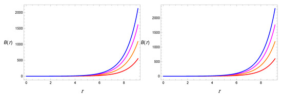
Figure 1.
Illustrates the variation behavior of , for , and under (★), (★), (★), (★), and .
4.2. Solution for
From Equation (25) we get the non-linear differential equation by taking as
By HPM scheme
consider
We considered the initial condition and where . The Equation (34) becomes with equating the powers of p.
This is a approximate solution for . The different developments can be seen from the right penal of the Figure 1, under the different values of parameter . The positively increasing behavior shows that our HPM solutions are physically considerable.
4.3. Solution for
By Equation (25) we have the following non-linear differential equation for as
By employing HPM scheme
we have
The initial condition can be freely picked. Here we set and where . The Equation (42), has following HPM setup
The approximate solution for . In this approximate solutions the parameter , has some important role. The different developments can be seen from the left penal of the Figure 2, under the different values of parameter . The increasing attribute shows that our HPM solutions are physically acceptable.
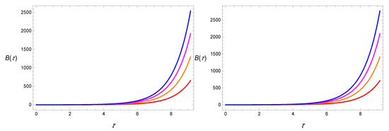
Figure 2.
Illustrates the variation behavior of , for , and under (★), (★), (★), (★), and .
4.4. Solution for
From above equation Equation (25) we have the following non-linear differential equation after putting the values of parameter as
Now, by using HPM scheme
This is a approximate solutions for , its graphically representation can be seen from the right side of the Figure 2.
4.5. Solution for
By Equation (25) with parameter we have the following non-linear equation
By employing HPM technique.
The approximate solution for . In this approximate solution, parameter has some important role. The different developments can be seen from the Figure 3, under the different values of parameter .
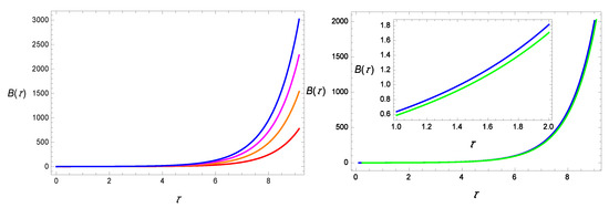
Figure 3.
Illustrates the variation behavior of , for under (★), (★), (★), (★), (★), , and .
4.6. Special Case
In this special case, we discuss the comparative study in the background of an exact solution of Equation (26) and HPM solution by Equation (33) with . The exact solution of Equation (26) is calculated as
where is a constant of integration. The comparison analysis of exact solution and HPM based solution can be seen from the right penal of from the Figure 3. We have also estimated the quantitative values of the exact solution for , which was possible to calculate and have shown these values in Table 1.

Table 1.
Estimated values for HPM and exact solutions.
5. Conclusions
In this article, we have studied the LRS Bianchi type-I space–time and calculated the fields equations. We have also calculated a cosmological model, which was presented in Equation (17). Further, we have developed an HPM scheme for a nonlinear differential equation. Furthermore, we have tried to find the solutions for the spatially modified cosmological model for LRS Bianchi type-I space–time, when the exact solution could not be found due to nonlinearity. In this response, we have examined the five different values of parameter n, i., and . We have also explored our solution for the four different values of parameter , i.e., and . Our obtained solutions can be seen from the Figure 1, Figure 2 and Figure 3 for five different cases. The variational development revealed that parameter n, has some special and important role in this study. Further, it is also noticed from Figure 1, Figure 2 and Figure 3 that parameter also has a crucial role in this modified cosmological problem. The increased values of parameter described the increased nature of our obtaining solutions. In our view, the results of the current study revealed that the HPM is very effective and simple for obtaining approximate solutions of the modified Friedmann equation in cosmology. Our purpose of this study is showing the applications of HMP in the cosmology field. In this study, we have obtained physically acceptable solutions with a positive nature, which support the study of HPM.
Author Contributions
Y.F.: Writing-original draft. L.H.: Writing-original draft. All authors have read and agreed to the published version of the manuscript.
Funding
This research was funded by the National Natural Science Foundation of China grant number 11271247; the Key Project of Support Program for Excellent Youth Talent in Colleges and Universities of Anhui Province grant number gxyqZD2016520; the Key Project for Natural Science Research of universities in Anhui Province grant numbers (KJ2015A347, KJ2017A702, KJ2019A1300); the Key Project for Teaching Research in Anhui Province grant numbers (2018jyxm0594, 2016jyxm0677, 2017jyxm0591); the Key Project of Teaching Research of Bozhou University grant number 2017zdjy02; and the Key Project of the Natural Science Research of Bozhou University grant numbers(BYZ2017B02,BYZ2017B03).
Conflicts of Interest
The authors declare that they have no known competing financial interests or personal relationships that could have appeared to influence the work reported in this paper.
References
- Morris, M.S.; Thorne, K.S. Wormholes in spacetime and their use for interstellar travel: A tool for teaching general relativity. Am. J. Phys. 1988, 56, 395–412. [Google Scholar] [CrossRef]
- Sharif, M.; Jawad, A. Phantom-like generalized cosmic chaplygin gas and traversable wormhole solutions. Eur. Phys. J. Plus 2014, 129, 15. [Google Scholar] [CrossRef]
- Lobo, F.S.N.; Parsaei, F.; Riazi, N. New asymptotically flat phantom wormhole solutions. Phys. Rev. D 2013, 87, 084030. [Google Scholar] [CrossRef]
- Kim, S.-W.; Lee, H. Exact solutions of a charged wormhole. Phys. Rev. D 2001, 63, 064014. [Google Scholar] [CrossRef]
- Copeland, E.J.; Sami, M.; Tsujikawa, S. Dynamics of Dark Energy. Int. J. Mod. Phys. D 2006, 15, 1753–1936. [Google Scholar] [CrossRef]
- De Leon, J.P. Mass and charge in brane-world and noncompact Kaluza-KLEin theories in 5 dim. Gen. Relativ. Gravit. 2003, 35, 1365–1384. [Google Scholar] [CrossRef]
- Landau, L.D.; Lifshitz, E.M. The Classical Theory of Fields, 3rd ed.; Pergamon Press: Oxford, UK, 1971; Volume 2. [Google Scholar]
- Sushkov, S.V.; Kim, S.W. Wormholes supported by the kink-like configuration of a scalar field. Class Quant Graw 2002, 19, 4909–4922. [Google Scholar] [CrossRef]
- He, J.H. Homotopy perturbation technique. Comput. Meth. Appl. Mech. Eng. 1999, 178, 257262. [Google Scholar] [CrossRef]
- Cveticanin, L. Homotopy-perturbation method for pure nonlinear differential equation. Chaos Solitons Fractals 2006, 30, 12211230. [Google Scholar] [CrossRef]
- He, J.H. Application of homotopy perturbation method to nonlinear wave equations. Chaos Solitons Fractals 2005, 26, 695700. [Google Scholar] [CrossRef]
- He, J.H. Limit cycle and bifurcation of nonlinear problems. Chaos Solitons Fractals 2005, 26, 827833. [Google Scholar] [CrossRef]
- He, J.H. Homotopy perturbation method for solving boundary value problems. Phys. Lett. A 2006, 350, 8788. [Google Scholar] [CrossRef]
- He, J.H. A coupling method of homotopy technique and perturbation technique for nonlinear problems. Int. J. Nonlinear Mech. 2000, 35, 3743. [Google Scholar] [CrossRef]
- He, J.H. Comparison of homotopy perturbation method and homotopy analysis method. Appl. Math. Comput. 2004, 156, 527539. [Google Scholar] [CrossRef]
- He, J.H. Homotopy perturbation method: A new nonlinear analytical technique. Appl. Math. Comput. 2003, 135, 7379. [Google Scholar] [CrossRef]
- He, J.H. Homotopy perturbation method with two expanding parameters. Indian J. Phys. 2014, 88, 193–196. [Google Scholar] [CrossRef]
- Farasat Shamir, M. Locally Rotationally Symmetric Bianchi Type I Cosmology in f(R,T) Gravity. Eur. Phys. J. C 2015, 75, 354. [Google Scholar] [CrossRef]
- Mustafa, G.; Abbas, G.; Shahzad, M.R.; Xia, T. Stable wormholes existence under non-commutative distributed background in Rastall theory. Can. J. Phys. 2019, 17, 0026. [Google Scholar] [CrossRef]
- Mustafa, G.; Shahzad, M.R.; Abbas, G.; Xia, T. Stable wormholes solutions in the background of Rastall theory. Mod. Phys. Lett. 2020, 33, 2050035. [Google Scholar] [CrossRef]


© 2020 by the authors. Licensee MDPI, Basel, Switzerland. This article is an open access article distributed under the terms and conditions of the Creative Commons Attribution (CC BY) license (http://creativecommons.org/licenses/by/4.0/).