Abstract
In several open and closed-loop systems, the trajectories converge to a region instead of an equilibrium point. Identifying the convergence region and proving the asymptotic convergence upon arbitrarily large initial values of the state variables are regarded as important issues. In this work, the convergence of the trajectories of a biological process is determined and proved via truncated functions and Barbalat’s Lemma, while a simple and systematic procedure is provided. The state variables of the process asymptotically converge to a compact set instead of an equilibrium point, with asymmetrical bounds of the compact sets. This convergence is rigorously proved by using asymmetric forms with vertex truncation for each state variable and the Barbalat’s lemma. This includes the definition of the truncated functions and the arrangement of its time derivative in terms of truncated functions. The proposed truncated function is different from the common one as it accounts for the model nonlinearities and the asymmetry of the vanishment region. The convergence analysis is valid for arbitrarily large initial values of the state variables, and arbitrarily large size of the convergence regions. The positive invariant nature of the convergence regions is proved. Simulations confirm the findings.
1. Introduction
In several open and closed loop systems, the trajectories converge to a region instead of an equilibrium point. Some examples are: (i) chaotic systems [1,2,3,4], (ii) systems that converge to limit cycles [5,6]; (iii) closed loop systems involving plant uncertainties [7,8,9,10,11]. The case of closed loop systems results majorly in adaptive control design for systems with model uncertainties and nonlinearities [8,9,10].
Identifying the convergence region of these systems and proving the asymptotic convergence upon arbitrarily large initial values of the state variables are regarded as important issues [1,5,12]. This stability analysis can be achieved via the following Lyapunov-function based approaches: the finite-time Lyapunov theory [8,9,10], the ultimate bound approach [13,14,15,16,17], and the Lyapunov-like function with vertex truncation approach [18,19]. For these approaches, the size of the target region is not constrained to be small, and cases with no equilibrium points can be considered. The Lyapunov function, its time derivative and the consequent convergence properties are important differences among them. An ideal stability analysis would be the direct extension of the stability analysis commonly used for systems converging to an equilibrium point, to the case of systems converging to a compact set. That is, a radially unbounded Lyapunov function is formulated so that its time derivative is upper bounded by a function that vanishes for the state variables being inside the convergence region, and it is negative otherwise. Then, the Barbalat’s Lemma is applied to prove the convergence of the state variables. The advantage of this analysis is its rigor, completeness and clarity. To the author’s knowledge, it is only developed in the Lyapunov-like function with vertex truncation approach, which is used for design of adaptive controllers, achieving the convergence of the tracking error to a compact set [11,18,19,20,21]. However, it is not well developed for open loop systems.
The finite-time Lyapunov theory is commonly applied for controller design, featuring the convergence of the tracking error of the closed loop system to a small target region within a well-defined time [8,9,10]. The fundamentals of the finite-time Lyapunov theory were originally given by Theorem 5.2 in [22]. The ultimate bound theory is commonly applied for chaotic systems. The system trajectories converge to attractive invariant sets that are properly identified [13,14,15,16,17]. The fundamentals of the used Lyapunov based theory were originally given by Leonov at the eighties, according to [3,15,16,17]. In these approaches, the Lyapunov function is formulated so that it appears in the right hand side of the expression of its time derivative. In this way, the Lyapunov function is monotonically decreasing and converges to a compact set, so that the state variables converge to some compact set. The required expression of the time derivative of the Lyapunov function can be obtained in some cases: (i) in open loop systems, e.g., chaotic attractors [13,14]; (ii) in controlled systems, by properly defining the control law [8,9,10,23]. Nevertheless, it is overly restrictive and overly difficult to obtain in other open loop systems.
Hence, a less restrictive approach is needed for proving the convergence of open loop systems to compact sets. To this end, in this work we prove the stability of a system comprising three differential equations, with a disturbance that induces the system to dwell around an equilibrium point, by proposing an extension of the Lyapunov-like function with vertex truncation approach. To the author’s knowledge, this is new to the current literature. This system arises from an open loop bioreaction model. The main contributions of this study are: (i) the asymptotic convergence of each state variable to a compact set of asymmetrical bounds is proved, using truncated forms and the Barbalat’s lemma; (ii) we propose a truncated form that is different to the common quadratic truncated form, as it involves the nonlinear reaction rate terms of the model and an asymmetrical vanishment region; (iii) the proof of asymptotic convergence holds for arbitrarily large initial values of the state variables, and arbitrarily large size of the convergence region; (iv) the invariance nature of the convergence sets is proved on the basis of the truncated forms.
The organization of the work is as follows. Section 2 presents the preliminary mathematical definitions (Section 2.1) an the model of the system (Section 2.2), expressing it in terms of its difference with respect to equilibrium conditions. Section 3 presents the main results of the stability analysis of a three dimension model with external disturbance. Section 4 presents the Lyapunov-based stability analysis of two simplified models. Section 4.1 considers a three dimension model with no external disturbances, whereas Section 4.2 considers a one-dimension model with external disturbance. Section 5 presents the detailed stability analysis of a three dimension model with external disturbance. In Section 6 a simulation example is presented. In Section 7 the conclusions are drawn.
2. Preliminary Definitions and Model Description
2.1. Preliminary Definitions
In this subsection, some mathematical expressions and terms used throughout this study are defined.
Compact set. A compact set is defined as , being , constant real numbers, and r the size of [8,24,25,26].
Boundedness. A scalar signal is bounded if there exists a constant such that for all [27].
Asymptotic convergence. The signal converges asymptotically to the region , if converges to as [28,29,30].
Remaining in a region. The signal remains in a region for , if for all [24,31,32].
The term ‘region’ corresponds to a set.
2.2. Model Description
We consider ammonification, nitrification, plant uptake and denitrification as the primary nitrogen removal and formation pathways. Ammonium is converted to nitrite in one step, whereas and are produced by nitrification and are consumed by denitrification [33,34]. Thus, the mass balance for nitrogen concentration across a single CSTR gives:
where is the concentration of organic nitrogen, and is its inflow concentration; is the concentration, and is its inflow concentration; is the concentration of nitrites plus nitrates, and is its inflow concentration. In addition, is the ammonification rate, is the nitrification rate, is the plant uptake rate, is the denitrification rate; is the inlet flowrate, is the outlet flow rate, V is the water volume. The effect of pH, temperature and dissolved oxygen are not considered, in order to facilitate the dynamic analysis. We use the following notation:
Thus, models (1) to (3) with functions (4) to (5) is rewritten as:
subject to the following features:
Characteristic 1.
, , , , , , are constant and positive.
Characteristic 2.
, are constant and positive.
Characteristic 3.
varies according to, whereis constant and positive, whereasis time varying and satisfies:; ; .
Characteristic 4.
, , remain in the region.
Now, we rewrite the model in terms of the equilibrium condition corresponding to . Subtracting the equilibrium condition from Equation (6), yields
Equation (11) follows from Characteristics 1 and 3. Subtracting the equilibrium condition from Equation (7), yields
The following properties hold:
Remark 1.
Characteristic 4 implies that , , remain in the region
3. Main Results
The stability analysis for a three dimension model with external disturbance includes: (i) definition of the truncated functions , what involves the choice of its gradient and the definition of the convergence regions ; (ii) determination of the time derivatives of the functions, what involves arranging the expressions in terms of functions; and (iii) determination of the boundedness, convergence and invariance properties of the state variables. The detailed procedure is presented in Section 5, whereas the main results are presented at what follows.
The gradient of the function is chosen to be:
where is defined as
The main properties of are:
Definition of the function:
whose main properties are
The time derivative of is:
By applying the Barbalat’s lemma, one obtains that converges asymptotically to .
The gradient of the function is chosen to be:
where is defined as
The main properties of are:
The function is defined as:
and its main properties are:
The linear combination of and gives:
By applying the Barbalat’s Lemma, one obtains that converges asymptotically to zero, and converges asymptotically to (23).
The gradient of the function is chosen to be:
where is defined as:
The main properties of are:
The definition of the function is:
and its main properties are:
The linear combination of , and gives:
By applying the Barbalat’s lemma, one obtains that convergences asymptotically to zero and to (25).
Proposition 1
Proposition 2
Proposition 3
(Invariance). Consider the system (6)–(8), subject to Characteristics 1 to 4, and signals (10), (20); (14), (13), (22); (18), (16), (24), and the sets (21), (23), (25). Let
The sets , , are positively invariant.
The proof of Proposition 1 is presented in Section 5.4, the proof of Proposition 2 is presented in Section 5.5, and the proof of Proposition 3 is presented in Section 5.6.
Remark 2.
The proposed , , functions allow to develop a rigorous and complete proof for the asymptotic convergence of , , to the compact sets , and , respectively, via the Barbalat’s lemma, taking into account the nonlinear terms of the model and the asymmetry of , and . To this end, the , and functions involve the nonlinear model terms and , and exhibit asymmetrical vanishment regions , and . Consequently, the linear combinations of the , and expressions involve the , , terms, which vanish for , and , respectively; then the Barbalat’s lemma can be applied in order to prove asymptotic convergence.
The main differences of the functions , , with respect to the common truncated quadratic form (e.g., [11,18]), are: (i) they involve the nonlinear asymmetrical functions ; (ii) the vanishment regions are asymmetrical, what renders asymmetrical.
Remark 3.
The proposed , and functions allow to develop a rigorous proof of positive invariance of the convergence sets , , . To this end, the characteristics of the , , expressions allow to obtain: for ; for and ; and for and .
4. Preliminary Results: Stability Analysis for Simplified Models
In this section, the asymptotic convergence of two simple systems is determined by using Lyapunov-like functions and functions with vertex truncation. The purpose is to provide the basic procedures of the stability analysis that will be developed later for a three dimension model with external disturbance. Section 4.1 considers a three-dimension system with no external disturbance, whereas Section 4.2 considers a one-dimensional system with an external disturbance. Truncated forms are only used in Section 4.2.
4.1. Three-Dimension Model with No External Disturbance
In this section, we determine the asymptotic convergence of the state variables of a three-dimension model with no external disturbances. Consider the model (9) to (18). In absence of disturbance, we have , so that and Equation (9) becomes:
The time derivative of the function satisfies:
Combining the above expressions, yields:
We impose the following condition on :
so that the definition of is:
whose main properties are:
Combining Equations (26) and (27), yields
This implies the asymptotic convergence of to zero, what is concluded by using the Barbalat’s Lemma on .
The time derivative of the function satisfies
Combining with Equation (12), yields
We impose the following condition on :
On the basis of this condition, the definition of the function is:
Its main properties are:
We consider the constant , that satisfies
Factorizing (31), arranging and multiplying by , yields
Adding this and Equation (28), yields
This implies the asymptotic convergence of to zero, what follows by using the Barbalat’s lemma on . Consequently, converges asymptotically to zero.
The time derivative of the function satisfies:
Combining with Equation (15), yields:
We impose the following condition on :
so that the definition of the function is:
and its main properties are:
We consider the constant , that satisfies:
Adding this and Equation (32), yields:
This implies the asymptotic convergence of to zero, what is concluded by using the Barbalat’s lemma on . Consequently, converges asymptotically to zero.
4.2. One-Dimension Model with External Disturbance
In this section, we determine and prove the asymptotic convergence of the state variable of a one-dimension system to a compact set of asymmetrical size. This stability analysis is based on the robust adaptive controller design that involves truncated forms (see [11,18]). In that approach, the Lyapunov function comprises a truncated quadratic form for the convergent state variable, and quadratic forms for other closed loop states. The truncated form exhibits a vanishment for values of the convergent state variable inside the convergence region. An early version of this type of functions is reported by [35], and later variants are reported by [11,18,19]. The time derivative of the Lyapunov function is an inequality in terms of the truncated quadratic form. The convergence of the convergent state variable is deduced by using the Barbalat’s Lemma, although the convergence time is not usually well-defined [11,21,36]. In this section, we apply the aforementioned approach to a one-dimension model with an external disturbance whose bounds are asymmetrical. To that end we propose a truncated form involving the nonlinear reaction rate terms and an asymmetrical vanishment region, instead of using the common truncated quadratic form.
Consider the system:
where k is constant and positive; is a time varying disturbance, satisfying , ; and is a function of that satisfies and . is defined in the region
Remark 4.
The bounds of are asymmetrical, that is , what implies that converges to a compact set of asymmetrical bounds.
The time derivative of the function V satisfies:
Combining this with Equation (37), yields
where d is a disturbance-like term satisfying , . We impose the following condition on the function V:
where is a truncated function that allows to prove the convergence of . To generate a proper expression of , we require to fulfill the following:
For the case , we have , therefore must be chosen such that for . This implies for . Thus, we choose
For the case we have . Therefore, must be chosen such that for . This implies for . Therefore, we choose:
The main properties of are:
On the basis of conditions (40) and (44), the definition of the function V is:
whose main properties are:
Remark 5.
The function V is not a Lyapunov function in the context of the definition used by [35] (p. 61), the main reason is that it is not positive definite, what is due to the truncation.
Remark 6.
The main differences of the function with respect to common truncated quadratic form (e.g., [11,18]) are: (i) it involves the nonlinear asymmetrical function which is a nonlinearity of the model; and (ii) the vanishment region Ω is asymmetrical, as , what renders asymmetrical. This structure allows us to develop a rigorous convergence proof, taking into account the nonlinear terms of the model and the asymmetry of the convergence set.
Integrating, yields
In view of properties (50), we have
This implies the asymptotic convergence of to zero, what can be proved by using the Barbalat’s Lemma [21,36] and properties (46) and (47). Consequently, converges asymptotically to (48).
Remark 7.
Due to the condition (40) and the definition of (44), V (49) exhibits vertex truncation, and the time derivative can be expressed in terms of the truncated quadratic form , see Equation (51). This allows to prove the asymptotic convergence of . V (49) and (44) have a common vanishment for (48), being the bounds of Ω asymmetrical.
Remark 8.
The validity of the proof of asymptotic convergence of is not disrupted by the following facts: (i) is defined in the region (38), so that its initial value can take arbitrarily large positive values; (ii) since δ can be arbitrarily large, then the size of the convergence region Ω (48) can be arbitrarily large.
5. Stability Analysis for the Case of Three Dimension Model with External Disturbance
In this section, the asymptotic convergence of a three dimension system with an external disturbance is determined by using functions with vertex truncation. The procedure is based on Section 4: (i) the dependence of the functions on the state variables and the addition of the expressions so as to obtain a non-positive nature is based on Section 4.1; (ii) the incorporation of truncation in the definition of the functions and the arrangement of ’s in terms of truncated forms is based on Section 4.2.
5.1. Stability Analysis for
Recall the differential equation for , that is, Equation (9). The time derivative of the function satisfies:
Substituting the expression (9) and arranging, yields
In view of characteristic 1 and Equation (10), is constant and positive. In view of (11), one further obtains , . Thus, in view of the term, we impose the following condition on :
where is a truncated function. On the basis of the procedure used in Section 4.2, we define it as
where , are defined as:
and the main properties of are:
On the basis of condition (53) and definition (54), the definition of the function is:
with properties
Using Property (57) yields:
This implies the asymptotic convergence of to zero, and to (61), as stated by Proposition 2. This is concluded by using the Barbalat’s Lemma [21,36].
Remark 9.
Remark 10.
The validity of the proof of asymptotic convergence of is not disrupted by the following facts: (i) is defined in the region , according to Remark 1, so that its initial value can take arbitrarily large positive values; (ii) since can be arbitrarily large, then (11) and the size of (61) can be arbitrarily large.
5.2. Stability Analysis for
Since Equation (12) involves the term , we need to express in terms of (54), which converges to zero as was already shown. Let
Therefore, can be expressed in terms of :
Substituting into Equation (12) and arranging, yields
where is defined in Equation (14). The time derivative of the function satisfies:
Combining with Equation (65) yields
Substituting (54) into (64) gives
since and are positive and constant, then , . In view of the term appearing in Equation (66), we impose the following condition on :
where is a truncated function, that we define as
where , are defined as:
The main properties of are:
On the basis of conditions (67) and (68), the definition of the function is:
where is defined in Equation (14). exhibits the properties
Using Property (71), yields
In view of the term , it is necessary to factorize and add the above expression with . We consider the constant , that satisfies
Factorizing the right hand side of (76), arranging and multiplying by , yields
Adding this and Equation (63), yields
This implies the asymptotic convergence of to zero, and to (74), as stated by Proposition 2.
Remark 11.
Remark 12.
The validity of the proof of asymptotic convergence ofis not disrupted by the following facts: (i)is defined in the region, according to Remark 1, so that its initial value can take arbitrarily large positive values; (ii) sincecan be arbitrarily large, then (11) and the size of (74) can be arbitrarily large.
5.3. Stability Analysis for
Recall that in Equation (15) the term is function of , being defined in Equation (17). Since converges to (74), then converges to a compact set satisfying
where
and , were defined in Equations (69) and (70). Thus, we express in terms of the truncated function , defined as:
The main properties of are:
In Equation (15), the term must be expressed in terms of . Let
Therefore, can be expressed in terms of and :
substituting this into Equation (15) and arranging, yields
where is defined in Equation (18). The time derivative of the function satisfies:
Combining with Equation (85), yields:
where is a disturbance-like term. Substituting (81) into (84) gives:
Therefore, , . In view of the term appearing in Equation (86), we impose the following condition on :
where is a truncated function, that we define as:
where satisfies properties (79) and (80), and , are defined as:
where
The main properties of are:
On the basis of conditions (87) and (88), the definition of the function is:
where is defined in Equation (18). exhibits the properties
Using property (91), yields
In view of the term , we need to factorize the term and to add the equations for , , . We consider the constant that satisfies
By using , the term can be rewritten as . In turn, the term can be factorized as
Using this property, Equation (96) can be expressed as:
Multiplying by and using property (83) on the term, yields
Adding this and Equation (78), yields
This implies the asymptotic convergence of to zero and to (94), as stated in Proposition 2.
Remark 13.
Remark 14.
The validity of the proof of asymptotic convergence of is not disrupted by the following facts: (i) is defined in the region , according to remark 1, so that its initial value can take arbitrarily large positive values; (ii) since can be arbitrarily large, then (11) and the size of (94) can be arbitrarily large.
5.4. Boundedness Analysis (Proof of Proposition 1)
To prove the boundedness of , we begin by arranging and integrating (63), what yields
To prove the boundedness of , we begin by arranging and integrating (78), what yields
To prove the boundedness of , we begin by arranging and integrating (97), what yields
5.5. Convergence Analysis (Proof of Proposition 2)
From (98) it follows that . It is necessary to prove that and to apply Barbalat’s Lemma. Recall that according to Proposition 1, hence . Differentiating with respect to time, using (54), yields:
where
Therefore
Thus, it follows from (101) that is well-defined and continuous with respect to . Recall that , according to Proposition 1. This and Equation (102) lead to .
Since , are bounded, it follows from (101) that is bounded. So far we have proved that , and . Thus, applying Barbalat’s lemma [27], yields . Hence, according to properties (59) and (60), converges asymptotically to .
From (99) it follows that . It is necessary to prove that and to apply Barbalat’s lemma. Recall that according to Proposition 1, hence . Differentiating with respect to time, using (68), yields:
where
Therefore,
Thus, is well-defined and continuous with respect to . Recall that , according to Proposition 1. This and Equations (104) and (105) lead to .
Since , are bounded, it follows from (103) that is bounded. So far we have proved that , and . Thus, applying Barbalat’s lemma [27], yields . Hence, according to properties (72) and (73), converges asymptotically to .
From (100) it follows that . It is necessary to prove that and to apply Barbalat’s lemma. Recall that according to proposition 1, hence . Differentiating with respect to time, using (88), yields:
Therefore,
5.6. Invariant Properties (Proof of Proposition 3)
The positive invariant nature of the convergence sets of , , is proved at what follows. A subset of the state space is positively invariant if the system trajectories starting inside it remain inside in the future. In addition, the positive invariant nature of a residual set is guaranteed if [37,38]. Consider the compact sets (61), (74) and (94). Let
According to Proposition 2,
Therefore, , , , , are attractive sets.
The set is positively invariant, what is concluded from:
what follows from Equation (63) and Property (59).
6. Example
We consider the model (1) to (3), with functions (4) to (5), subject to Characteristics 1–4, and with the following parameter values, based on [33]:
Therefore, day, day.
We consider mg/L, days. Therefore, max .
Using Equations (6)–(8), we obtain the following equilibrium points: mg/L, mg/L, mg/L. From Equations (55) and (56) it follows that , . From Equations (69) and (70) it follows that , . From Equations (89) and (90) it follows that , .
Figure 1 presents the time course of , , . The lower and upper bounds of the convergence regions, that is, , , , , , are shown as horizontal dashed-lines. It can be noticed that once the trajectories enter the compact set , they remain inside it.
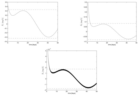
Figure 1.
Time course of (upper left), (upper right), (lower left). The lower and upper bounds of the convergence regions, that is, , , , , , are shown as horizontal dashed-lines.
7. Discussion
It was shown that the asymptotic stability of the bioreaction process considered can be proved by using functions with vertex truncation. The size of the convergence region of the state variables depend on the bounds of the external disturbance. This size can be large, and far from the equilibrium point. A simple and systematic procedure was provided to determine and prove asymptotic convergence of the state variables towards a compact set of asymmetrical bounds, what includes definition of the truncated functions and the truncated forms appearing in its time derivative. Both of these truncated functions exhibit a vanishment for values of the state variables in the convergence region. The analysis is valid for arbitrarily large positive initial values of the state variables, and arbitrarily large size of the convergence regions. The stability analysis was based on that of classical robust adaptive controller design, but the truncated function was different to the common truncated quadratic function, as it involves the model nonlinearities and an asymmetrical vanishment region.
Although the approach was developed for a specific biological process, it can be adapted to other systems, including systems converging to limit cycles.
Author Contributions
Conceptualization, methodology and writing of the original draft, A.R.; writing—review and editing, G.O. and G.Y.F. All authors have read and agree to the published version of the manuscript.
Funding
A. Rincón and GY. Florez were funded by Universidad Católica de Manizales.
Acknowledgments
G. Olivar thanks Colciencias for supporting the publication of this paper through the project “Modelado y simulación del Metabolismo Urbano de Bogotá D.C. Código 111974558276”.
Conflicts of Interest
The authors declare no conflict of interests regarding the publication of this paper. The funders had no role in the design of the study, analysis, interpretation of results or writing of the manuscript.
References
- Zhou, G.; Liao, X.; Xu, B.; Yu, P.; Chen, G. Simple algebraic necessary and sufficient conditions for Lyapunov stability of a Chen system and their applications. Trans. Inst. Meas. Control. 2018, 40, 2200–2210. [Google Scholar] [CrossRef]
- Liao, X.; Fu, Y.; Xie, S. On the new results of global attractive set and positive invariant set of the Lorenz chaotic system and the applications to chaos control and synchronization. Sci. China Ser. F Inf. Sci. 2005, 48, 304–321. [Google Scholar] [CrossRef]
- Yu, P.; Liao, X. Globally attractive and positive invariant set of the Lorenz system. Int. J. Bifurc. Chaos 2006, 16, 757–764. [Google Scholar] [CrossRef]
- Li, D.; Lu, J.; Wu, X.; Chen, G. Estimating the bounds for the Lorenz family of chaotic systems. Chaos Solitons Fractals 2005, 23, 529–534. [Google Scholar] [CrossRef]
- Ratschan, S.; She, Z. Providing a basin of attraction to a target region of polynomial systems by computation of Lypunov-like functions. SIAM J. Control Optim. 2010, 48, 4377–4394. [Google Scholar] [CrossRef]
- Papachristodoulou, A.; Prajna, S. On the construction of lyapunov functions using the sum of squares decomposition. In Proceedings of the 41st IEEE Conference on Decision and Control, Las Vegas, NV, USA, 10–13 December 2002; pp. 3482–3487. [Google Scholar]
- Liu, Z.; Wang, F.; Zhang, Y.; Philip Chen, C.L. Fuzzy adaptive quantized control for a class of stochastic nonlinear uncertain systems. IEEE Trans. Cybern. 2016, 46, 524–534. [Google Scholar] [CrossRef]
- Boulkroune, A.; Msaad, M.; Farza, M. Adaptive fuzzy system-based variable-structure controller for multivariable nonaffine nonlinear uncertain systems subject to actuator nonlinearities. Neural Comput. Appl. 2017, 28, 3371–3384. [Google Scholar] [CrossRef]
- Cai, M.; Xiang, Z. Adaptive practical finite-time stabilization for uncertain nonstrict feedback nonlinear systems with input nonlinearity. IEEE Trans. Syst. Man Cybern. Syst. 2017, 47, 1668–1678. [Google Scholar] [CrossRef]
- Zhu, Z.; Xia, Y.; Fu, M. Attitude stabilization of rigid spacecraft with finite-time convergence. Int. J. Robust Nonlinear Control 2011, 21, 686–702. [Google Scholar] [CrossRef]
- Rincon, A.; Piarpuzán, D.; Angulo, F. A new adaptive controller for bio-reactors with unknown kinetics and biomass concentration: Guarantees for the boundedness and convergence properties. Math. Comput. Simul. 2015, 112, 1–13. [Google Scholar] [CrossRef]
- Meadows, T.; Weedermann, M.; Wolkowicz, G.S.K. Global analysis of a simplified model of anaerobic digestion and a new result for the chemostat. SIAM J. Appl. Math. 2019, 79, 668–689. [Google Scholar] [CrossRef]
- Zhang, F.; Liao, X.; Zhang, G.; Mu, C. Dynamical analysis of the generalized Lorenz systems. J. Dyn. Control Syst. 2017, 23, 349–362. [Google Scholar] [CrossRef]
- Zhang, F.; Liao, X.; Zhang, G. On the global boundedness of the Lü system. Appl. Math. Comput. 2016, 284, 332–339. [Google Scholar] [CrossRef]
- Liao, X.; Zhou, G.; Yang, Q.; Fu, Y.; Chen, G. Constructive proof of Lagrange stability and sufficient—Necessary conditions of Lyapunov stability for Yang–Chen chaotic system. Appl. Math. Comput. 2017, 309, 205–221. [Google Scholar] [CrossRef]
- Zhang, F.; Mu, C.; Wang, L.; Zhang, G.; Ahmed, I. On the new results of global exponential attractive set. Appl. Math. Lett. 2014, 28, 30–37. [Google Scholar] [CrossRef]
- Mu, C.; Zhang, F.; Shu, Y. On the boundedness of solutions to the Lorenz-like family of chaotic systems. Nonlinear Dyn. 2012, 67, 987–996. [Google Scholar] [CrossRef]
- Su, C.; Feng, Y.; Hong, H.; Chen, X. Adaptive control of system involving complex hysteretic nonlinearities: A generalised Prandtl–Ishlinskii modelling approach. Int. J. Control 2009, 82, 1786–1793. [Google Scholar] [CrossRef]
- Zhou, J.; Zhang, C.; Wen, C. Robust adaptive output control of uncertain nonlinear plants with unknown backlash nonlinearity. IEEE Trans. Autom. Control 2007, 52, 503–509. [Google Scholar] [CrossRef]
- Zhou, J.; Wen, C.; Zhang, Y. Adaptive output control of nonlinear systems with uncertain dead-zone nonlinearity. IEEE Trans. Autom. Control 2006, 51, 504–511. [Google Scholar] [CrossRef]
- Koo, K. Stable adaptive fuzzy controller with time-varying dead-zone. Fuzzy Sets Syst. 2001, 121, 161–168. [Google Scholar] [CrossRef]
- Bhat, S.; Bernstein, D. Finite-time stability of continuous autonomous systems. SIAM J. Control Optim. 2000, 38, 751–766. [Google Scholar] [CrossRef]
- Jian, J.; Deng, X.; Tu, Z. New results of globally exponentially attractive set and synchronization controlling of the Qi chaotic system. In Advances in Neural Networks—ISNN 2010; Zhang, L., Kwok, J., Lu, B.L., Eds.; Springer: Berlin, Germany, 2010; pp. 643–650. [Google Scholar]
- Yao, B.; Tomizuka, M. Adaptive robust control of SISO nonlinear systems in a semi-strict feedback form. Automatica 1997, 33, 893–900. [Google Scholar] [CrossRef]
- Gao, S.; Ning, B.; Dong, H. Fuzzy dynamic surface control for uncertain nonlinear systems under input saturation via truncated adaptation approach. Fuzzy Sets Syst. 2016, 290, 100–117. [Google Scholar] [CrossRef]
- Cao, C.; Hovakimyan, N. Design and analysis of a novel L1 adaptive control architecture with guaranteed transient performance. IEEE Trans. Autom. Control 2008, 53, 586–591. [Google Scholar] [CrossRef]
- Ioannou, P.; Sun, J. Robust Adaptive Control; Prentice-Hall PTR: Upper Saddle River, NJ, USA, 1996. [Google Scholar]
- Wang, X.; Su, C.; Hong, H. Robust adaptive control of a class of nonlinear systems with unknown dead-zone. Automatica 2004, 40, 407–413. [Google Scholar] [CrossRef]
- Zhou, J.; Wen, C.; Zhang, Y. Adaptive backstepping control of a class of uncertain nonlinear systems with unknown backlash-like hysteresis. IEEE Trans. Autom. Control 2004, 49, 1751–1757. [Google Scholar] [CrossRef]
- Wang, Q.; Su, C. Robust adaptive control of a class of nonlinear systems including actuator hysteresis with Prandtl–Ishlinskii presentations. Automatica 2006, 42, 859–867. [Google Scholar] [CrossRef]
- Ge, S.S.; Hang, C.C.; Zhang, T. Adaptive neural network control of nonlinear systems by state and output feedback. IEEE Trans. Syst. Man Cybern. -Part B Cybern. 1999, 29, 818–828. [Google Scholar] [CrossRef]
- Ioannou, P.; Kokotovic, P. Robust redesign of adaptive control. IEEE Trans. Autom. Control 1984, AC-29, 202–211. [Google Scholar] [CrossRef]
- Xuan, Z.; Chang, N.; Daranpob, A.; Wanielista, M. Modeling subsurface upflow wetland systems for wastewater effluent treatment. Environ. Eng. Sci. 2010, 27, 879–888. [Google Scholar] [CrossRef]
- Ramírez-León, H.; Barrios-Piña, H.; Cuevas-Otero, A.; Torres-Bejarano, F.; Ponce-Palafox, J. Hydraulic and environmental design of a constructed wetland as a treatment for shrimp aquaculture effluents. In High Performance Computer Applications; Gitler, I., Klapp, J., Eds.; Springer: Berlin, Germany, 2015; pp. 508–522. [Google Scholar]
- Slotine, J.; Li, W. Applied Nonlinear Control; Prentice-Hall Inc.: Upper Saddle River, NJ, USA, 1991. [Google Scholar]
- Su, C.; Stepanenko, Y.; Svoboda, J.; Leung, T.P. Robust adaptive control of a class of nonlinear systems with unknown backlash-like hysteresis. IEEE Trans. Autom. Control 2000, 45, 2427–2432. [Google Scholar] [CrossRef]
- Blanchini, F. Set invariance in control. Automatica 1999, 35, 1747–1767. [Google Scholar] [CrossRef]
- Cao, Y.-Y.; Lin, Z.; Ward, D.G. Anti-windup design of output tracking systems subject to actuator saturation and constant disturbances. Automatica 2004, 40, 1221–1228. [Google Scholar] [CrossRef]

© 2020 by the authors. Licensee MDPI, Basel, Switzerland. This article is an open access article distributed under the terms and conditions of the Creative Commons Attribution (CC BY) license (http://creativecommons.org/licenses/by/4.0/).