The Impact of Nanoparticles Due to Applied Magnetic Dipole in Micropolar Fluid Flow Using the Finite Element Method

Abstract

The present work examines the effect of different magnetic nanoparticles and the heat transfer phenomena over the stretching sheet with thermal stratification and slips effect. The mixture of water (H${}_2$O) and ethylene glycol (C${}_2$H${}_6$O${}_2$) is used as base fluid whereas the paramagnetic, diamagnetic, and ferromagnetic ferrites are taken as nanoparticles. In the presence of ferrite nanoparticles, the magnetic dipole has a significant effect in controlling the rate of heat transfer and the thermal boundary layers. By using suitable similarity transformations, the system of partial differential equations is transformed into nonlinear ordinary differential equations. The numerical solution of resulting equations is found out by using the variational finite element method. The effect of numerous emerging parameters on velocity, temperature, and micro-rotation velocity are represented graphically and analyzed numerically. It has been noticed that comparatively the diamagnetic ferrites have gained maximum thermal conductivity relative to the other nanoparticles. It was also observed that the thermal conduction of nanoparticles increases with the variation of volume fraction. Moreover, with increasing values of thermal stratification the thermal boundary layer thickness decreases and the heat transfer rate increases at the surface. Furthermore, the validation of code and the accuracy of the numerical technique has been confirmed by the assessment of current results with earlier studies.

1. Introduction

The Heat transfer enrichment in the two-phase fluid flow has been inspected for several years. Due to the truncated thermal conductivity of fluids, the foremost heat transfer mechanism between them is deliberated as convection. Research on nano-fluid flow demonstrates that by adding ferrite nanoparticles into the fluid, the coefficient of heat transfer can be increased. The resulting intensification in the heat transfer, in addition to the probable escalation in thermal conductivity, was mainly because of the condensed thickness of the thermal boundary layer. The examples of significant usages of heat transfer liquids containing hydronic and cooling heating systems in buildings, the vehicular and avionic cooling system in industries, chemical, nutrients, and other processing plants [1,2,3,4]. The scholars have investigated to apprize the potentiality for the ferrofluid applications in the fast-developing fields of micro-electromechanical systems (MEMS) and nano-electromechanical systems (NEMS), because of small spherical diameter (10 nm) of the perpetually magnetized nanoparticles. The basic idea of nanofluid is to increase the thermal conductivity of the base fluid by the diffusion of nanometer-scaled dense particles into fluids, these dense particles are of various kinds of material like metal oxides, metals, etc. Moreover, there are numerous applications in engineering and industries related to the boundary layer flow over a stretching sheet-like as crystal growing and paper production; more applications of stretching sheet may be seen in the articles [5,6]. Crane [7] has inspected the fluid flow over the stretching sheet after that on condensed to non-newtonian fluids. Sarafraz et al. [8] were investigated experimentally about the flow sweltering heat transference of zirconia water nanofluid inside a heat exchanger. Magnetic nanoparticles are characteristically organized in various sizes and morphologies from metallic materials such as sapphire, nickel, iron, and their oxides as an example, magnetite (Fe${}_3$O${}_4$) and spinel-type ferrites [9].

The properties of magnetic and thermal filed gradients on drenched ferrofluid flow was scrutinized by Neuringer et al. [10]. The transportation of heat phenomena causes of stretching sheets via ambient fluids is stated and categorized widely analysis in contemporary literature. Ferro-fluids are fluids that are manufactured through a non-natural approach and composite of immensely abbreviated colloid deferments of well and thin magnetic-particles in the non-conducting transporter fluids. Sharma et al. [11] stated the effect of dust particles in the ferromagnetic fluid with thermal convection. Mee [12] dissected a technique with ferrofluids that can be used to detention the magnetic protectorate edifices on the surface of ferrofluids in the existence of a magnetic dipole. Furthermore, the ferrofluids are liquids that are reproduced artificially and exposed to extremely condensed colloid suspension of fine and reedy magnetic particles in a non-conducting carter fluid. Nadeem et al. [13] exemplified the effect of the magnetic dipole over a permeable medium in the flow of ferrofluid. Sheikholeslami et al. [14] inspected that the free convection of a magnetic nanofluid in a porous curved hollow under the consequence of an exterior magnetic source. Madhu and Kishan [15] examined the heat and mass transfer rate by magnetohydrodynamic mixed convection stagnation point flow of a non-Newtonian power-law nanofluid through the stretching surface with the existence of radiation by using the finite element method. Presently, Bognar et al. [16] scrutinized the magneto thermo-mechanical implications regarding the heated dense incompressible ferrofluid and the cold wall in the existence of a variable magnetic field. Ali et al. [17] have explored the steady magnetohydrodynamic of the axisymmetric flow of incompressible, viscid, electrically-conducted nanofluid with convective boundary conditions and thermo-diffusion through a radially stretched sheet.

Ferrofluids are the mixture of nanoparticles and liquids, prepared for ferromagnetic ferrites dialect in an electrically nonconducting transporter fluid. Recently, the philosophy of microfluidics has been found remarkable consideration, as the Newtonian-fluids cannot classify the characteristics of fluids with suspended elements. Li et al. [18] explored the impacts of element volume fraction, surfactant and the magnetic field that proceeding the transference properties of water-based Fe magnetic nano-fluid. Liaqat et al. [19] examined the effect of viscous dissipation and the various sorts of magnetic nano-particles, ferromagnetic and ferrimagnetic, on micropolar fluid flow and heat transfer through the stretching sheet. Yirga and Tesfay [20] deliberated about the heat, and mass transference study of nano-fluid over the porous stretching sheet. The authors revealed that Ag water nano-fluid has larger skin friction as associated with Cu water nano-fluid. Some further applications that appropriates the flow of liquors possibly found in [21,22]. Liaqat et al. [23] explore the influences of multi-slip and solutal boundary conditions on magnetohydrodynamic unsteady bioconvective micropolar nano-fluid restrictive gyrotactic micro-organism, mass and heat transfer impact through a sheet. Multiple slip impacts on magnetohydrodynamic unsteady viscoelastic nanofluid flow with radiation through a penetrable stretching sheet using the finite element method was discussed by Khan et al. [24]. Turkyilmazoglu [25] has analyzed about the heat transfer and also about the micropolar fluid flow passed through the stretching sheet. M.S. Shadloo et al. [26] studied a two-dimensional steady convective micropolar fluid flow through a stretching sheet in the existence of radiation and constant temperature. Pradhan et al. [27] analysis is carried out for the free convective fluid flow via an electrically directed micropolar fluid through a permeable stretching sheet in the appearance of the absorbent medium. Mehdi Bahiraei et al. [28] was examined about the thermo-hydraulic features of the green graphene nanoplatelets nanofluid through the tube prepared with the rotating twisted tape. Eringen [29] described a philosophy of micropolar fluid that cannot be explained by classical Navier stokes equations cause of micro inertia and gyration or microgyration impacts. Ahmadi [30] describes the self-similar consequences of the incompressible micropolar boundary layer flow through the semi-infinite plate. Gorla [31] signified a study on micropolar boundary layer flow at the stagnation point on the moving wall. Ibrahim and Shankar [32] reveal that the heat transfer and the magnetohydrodynamic boundary layer flow of nanofluids via inflatable stretching sheet with velocity, thermal, and solutal-slip boundary conditions. Das [33] explored a very imperious numerical study on the convective heat transfer narration of nano-fluids over an infiltrate-able stretching sheet in the presence of partial slip, thermal buoyancy, and internal heat development. Abbas et al. [34] premeditated the impacts of radiation in the existence of a similar magnetic field for nano-fluids on a frizzed stretching sheet by assimilating the consequences of slip. Sohaib Abdal et al. [35] inspected the multislip effects on the magnetohydrodynamics mixed convection unsteady flow of micropolar nanofluid over a stretching/shrinking sheet in the presence of heat source and radiation.

In spite of all the above literature, it is described that the former investigators have focused on ferrofluid flows over a stretching sheet without thermal stratification and slips effect in the presence of a magnetic dipole. This research is to scrutinize the behavior of various ferrite nanoparticles and their thermal conductivity on boundary layer slip flow and the heat transfer phenomena. The nanoparticles Ta (Paramagnetic), Cu (Diamagnetic), Fe (Ferromagnetic) as ferrites of nanoparticles and the mixture of water H${}_2$O and ethylene glycol (C${}_2$H${}_6$O${}_2$) are used as base fluids. The phenomena of thermal stratification and slips effect in the presence of a magnetic dipole have been taken into consideration. Moreover, we inspect the behavior of different sorts of magnetic nanoparticles, emerging physical parameters and thermal conductivity graphically by a detailed discussion. Furthermore, the numerical estimations of current results are shown in tables with diagrams.

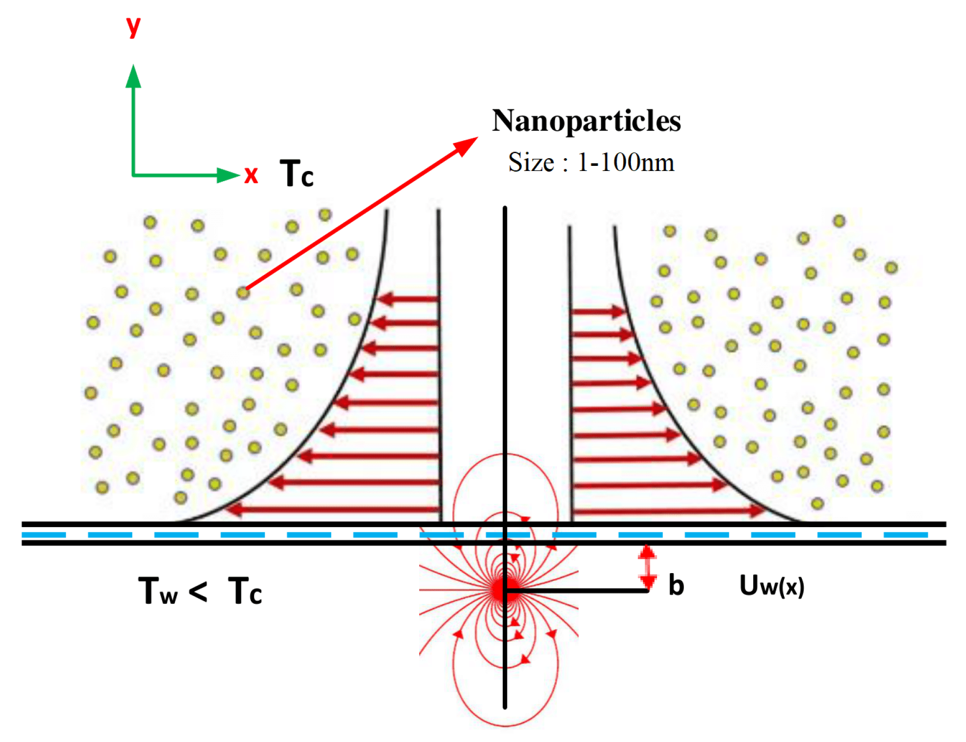
2. Problem Description

Consider a two-dimensional magnetohydrodynamic, incompressible, boundary layer, micropolar magnetic nanofluid flow over an electrically non-conducted stretching surface. The magnetic nanofluid contains paramagnetic, diamagnetic and ferromagnetic as nanoparticles suspended with water H${}_2$O and ethylene glycol C${}_2$H${}_6$O${}_2$ as a conventional fluid through a stretching sheet. The dimensions of the surface have been chosen along the x-axis and y-axis. $u_w=cx$ is the velocity of the sheet as exposed in Figure 1. Moreover, the magnetic dipole is situated in such a way that its midpoint is accurately located on the y-axis at a distance of b from the x-axis. The field points of the magnetic dipole are applied in the positive x-axis. The temperature $T_w$ at the stretching sheet is lesser than the cure temperature and is supposed to be $T_c$, the temperature $T=T_{\infty }$ is considered as the temperature of fluid away from the surface, where $T_c>T_{\infty }>T_w$ and the fluid that is away from $T_c$ is unable of being magnetized. The variable temperature $T_w=T_0+b_{1}x$ is considered at the surface and is $T_{\infty }=T_0+b_{2}x$, away from the surface. The leading equations for flow can be stated as [36].

$$\frac{\partial u}{\partial x}+\frac{\partial v}{\partial y}=0,$$

(1)

$$u\frac{\partial u}{\partial x}+v\frac{\partial u}{\partial y}=\frac{{\mu }_0}{\rho }M\frac{\partial H}{\partial x}+\left(\frac{{\mu }_{nf}+\kappa }{{\rho }_{nf}}\right)\frac{{\partial }^{2}u}{\partial y^2}+\frac{\kappa }{{\rho }_{nf}}\frac{\partial w}{\partial y},$$

(2)

$$u\frac{\partial w}{\partial x}+v\frac{\partial w}{\partial y}=\frac{{\gamma }_{nf}}{({\rho }_{nf})j}\frac{{\partial }^{2}w}{\partial y^2}-\frac{\kappa }{({\rho }_{nf})j}\left(2w+\frac{\partial u}{\partial y}\right),$$

(3)

$$u\frac{\partial T}{\partial x}+v\frac{\partial T}{\partial y}+\left(u\frac{\partial H}{\partial x}+v\frac{\partial H}{\partial y}\right)\frac{{\mu }_0}{{({\rho }_{cp})}_{nf}}T\frac{\partial M}{\partial T}={\alpha }_{nf}\frac{{\partial }^{2}T}{\partial y^2}-\frac{\partial q_r}{\partial y}+\frac{{\mu }_{nf}}{{({\rho }_{cp})}_{nf}}[{(\frac{\partial u}{\partial y})}^2+2(\frac{\partial v}{\partial y}{)}^2]$$

(4)

where $(u,v)$ are the components of velocity along the x-axis and y-axis, respectively. ${\alpha }_{nf}$ is the normal anxiety moduli, ${\rho }_{nf}$ is the fluid density, and ${\mu }_{nf}$ describes the dynamic viscosity of the fluid, respectively. Further, M shows the magnetization, H is magnetic penetrability, ${\mu }_0$ denotes the magnetic field, and ${({\rho }_{cp})}_{nf}$ are the thermal capability of nano-fluid, separately. In Equation (3), the spin gradient viscosity is ${\gamma }_{nf}$, and is expressed as $\gamma =\sqrt{S\rho b^2}/\sqrt{\mu }$ where b is constant, and in Equation (4) $q_r$ is the heat flux, that is explained as $q_r=-\frac{4{\sigma }^{*}}{3{\kappa }^{*}}\frac{\partial T^4}{\partial y}$ where Stefan-Boltzmann number is ${\sigma }^{*}$ and the mean assimilation coefficient is ${\kappa }^{*}$. The thermo-physical factors are explained as [37].

$$\begin{array}{ccc}\hfill {\alpha }_1& =& {\rho }_{nf}={(1-\varphi )}_{\rho f}+\varphi {\rho }_s,{\alpha }_2={\mu }_{nf}=\frac{{\mu }_f}{{(1-\varphi )}^{2.5}},\hfill \\ \hfill {\alpha }_3& =& {(\rho C_p)}_{nf}=(1-\varphi ){(\rho C_p)}_f+\varphi {(\rho C_p)}_s,{\alpha }_4=\frac{{\kappa }_{nf}}{{\kappa }_f}=\frac{({\kappa }_s+2{\kappa }_f)-2\varphi ({\kappa }_f-{\kappa }_s)}{({\kappa }_s+2{\kappa }_f)+\varphi ({\kappa }_f-{\kappa }_s)}.\hfill \end{array}$$

The boundary conditions for the stated mathematical model are detailed as

$$\begin{array}{c}u=u_w(x)+A_1\frac{\partial u}{\partial y},v=-v_w,T=T_w=T_0+b_{1}x,w=-\delta \frac{\partial u}{\partial y},asy=0.\\ u=0,w=0,T\to T_{\infty }=T_0+b_{2}x,asy\to \infty .\end{array}$$

(5)

where $T_0$, $b_1$, and $b_2$ are allude temperature and dimensionless quantities respectively, $\varphi$ is solid volume fraction, ${\kappa }_s$ and ${\kappa }_f$ are respective thermal conductivities of the nanoparticles and the base fluids, and ${\rho }_s$ and ${\rho }_f$ are respective densities of the nanoparticles and the base fluid. The temperature $T_w$ at the surface, $T_c$ is Curie temperature, $T_{\infty }$ temperature of fluid away from the surface and $A_1$ is the velocity slip parameter.

The magnetic nanofluid flow is affected through the dipole field utilizing magnetic scalar potential $\tau$ such as, ([38])

$$\tau =(\frac{\gamma }{2\pi })x/(x^2+{(y+b)}^2)$$

(6)

The strength of magnetic field at the source position is represented by $\gamma$ and b denotes the distance from x-axis to the centre of magnetic field, and the x, y components of magnetic field M are shown as

$$M_x=-\partial \tau /\partial x=(\frac{\gamma }{2\pi })(x^2-{(y+b)}^2)/{(x^2+{(y+b)}^2)}^2$$

(7)

$$M_y=-\partial \tau /\partial y=(\frac{\gamma }{2\pi })(2x(y+c))/{(x^2+{(y+c)}^2)}^2$$

(8)

as the force of body is proportionated to the gradient of magnitude M which is

$$M=\sqrt{{(\partial \tau /\partial x)}^2+{(\partial \tau /\partial y)}^2}$$

(9)

By using Equations (7) and (8) to solve Equation (9) by expanding power of x up to $x^2$, then we get

$$\partial M/\partial x=-\frac{\gamma }{2\pi }(2x/{(y+b)}^4)$$

(10)

$$\partial M/\partial y=\frac{\gamma }{2\pi }(-2/{(y+b)}^3+4x^2/{(y+b)}^5)$$

(11)

With temperature T, the impact of magnetization M is expressed as $M=K_1(T-T\infty )$, where $K_1$ shows pyromagnetic coefficient. To solve the system of equations, we are substituting the similarity transformations; [38]

$$\psi (\eta ,\zeta )=(\mu /\rho )\eta \tilde{f}(\zeta ),\theta (\eta ,\zeta )=(T_{\infty }-T)/(T_0-T_w)={\tilde{\theta }}_1(\zeta )+{\eta }^2{\tilde{\theta }}_2(\zeta )$$

(12)

where $\mu$ symbolize dynamic viscosity, ${\tilde{\theta }}_1(\zeta )$, ${\tilde{\theta }}_2(\zeta )$ symbolize the dimensionless temperature respectively, and the non dimensional co-ordinates are as;

$$\zeta =y\sqrt{(c{\rho }_f)/{\mu }_f},\eta =x\sqrt{(c{\rho }_f)/{\mu }_f},\omega =cx\sqrt{\frac{c\mu }{\rho }}\tilde{g}(\zeta )$$

(13)

The components of velocity for the stream function $\psi (\eta ,\zeta )$ and for temperature $\tilde{\theta }(\eta ,\zeta )$ are,

$$u=\frac{\partial \psi }{\partial y}=cx{\tilde{f}}^{\prime }(\zeta ),v=-\frac{\partial \psi }{\partial x}=-\sqrt{(c{v}_f)}\tilde{f}(\zeta ),$$

(14)

According to similarity transformations Equations (12)–(14), the system of equations from (1)–(4) are transformed into system of ordinary differential equations (ODEs):

$$({\alpha }_5+K)\frac{d^3\tilde{f}}{d{\zeta }^3}-{\alpha }_1{\left(\frac{d\tilde{f}}{d\zeta }\right)}^2+{\alpha }_1\tilde{f}\frac{d^2\tilde{f}}{d{\zeta }^2}+K\frac{d\tilde{g}}{d\zeta }-\frac{2\beta {\tilde{\theta }}_1}{{(\zeta +\gamma )}^4}=0,$$

(15)

$$({\alpha }_5+K/2)\frac{d^2\tilde{g}}{d{\zeta }^2}-{\alpha }_1\tilde{f}\frac{d\tilde{g}}{d\zeta }+{\alpha }_1\tilde{g}\frac{d\tilde{f}}{d\zeta }-K\left(2\tilde{g}+\frac{d^2\tilde{f}}{d{\zeta }^2}\right)=0,$$

(16)

$${\alpha }_4(1+Rd)\frac{d^2{\tilde{\theta }}_1}{d{\zeta }^2}+{\alpha }_{3}Pr\left(f\frac{d{\tilde{\theta }}_1}{d\zeta }-2{\tilde{\theta }}_1\frac{d\tilde{f}}{d\zeta }\right)+\frac{2\lambda \beta \tilde{f}({\tilde{\theta }}_1-ϵ)}{{(\zeta +\gamma )}^3}-2\lambda {\alpha }_5{\left(\frac{d\tilde{f}}{d\zeta }\right)}^2=0,$$

(17)

$${\alpha }_4(1+Rd)\frac{d^2{\tilde{\theta }}_2}{d{\zeta }^2}+{\alpha }_{3}Pr\left(\tilde{f}\frac{d{\tilde{\theta }}_2}{d\zeta }-4{\tilde{\theta }}_2\frac{d\tilde{f}}{d\zeta }\right)+\frac{2\lambda \beta {\tilde{\theta }}_2}{{(\zeta +\gamma )}^3}$$

$$-\lambda \beta ({\tilde{\theta }}_1-ϵ)\left[\frac{2}{{(\zeta +\gamma )}^4}\frac{d\tilde{f}}{d\zeta }+\frac{4\tilde{f}}{{(\zeta +\gamma )}^5}\right]-\lambda {\alpha }_5{\left(\frac{d^2\tilde{f}}{d{\zeta }^2}\right)}^2=0,$$

(18)

for the above problem the transformed boundary conditions are:

$$\tilde{f}(0)=f_w,\frac{d\tilde{f}(0)}{d\zeta }=1+S_f\frac{d{\tilde{f}}^2(0)}{d{\zeta }^2},\tilde{g}(0)=-\delta \frac{d^2\tilde{f}(0)}{d{\zeta }^2},{\tilde{\theta }}_1=1-S_1,and{\tilde{\theta }}_2=0.$$

(19)

$$\frac{d\tilde{f}(\infty )}{d\zeta }\to 0,\tilde{g}\to 0,{\tilde{\theta }}_1(\infty )\to 0,and{\tilde{\theta }}_2(\infty )\to 0.$$

(20)

The primes show the derivatives with respect to the variable $\zeta$. The involving parameters in Equations (15)–(18) are explained as: $P_r=\nu /\alpha$, $S_1=b_2/b_1$ $ϵ=T_{\infty }/T_0-T_w$, $\beta =\frac{\gamma }{2\pi }\frac{K{\mu }_0(T_0-T_w)\rho }{{\mu }_0^2}$, $\delta =A{(\frac{c\mu }{\rho })}^{1/2}$ $\lambda =c{\mu }^2/\rho \kappa (T_0-T_w)$, $\gamma =\sqrt{c\rho b^2}/\sqrt{\mu }$ $S_f=\sqrt{(c{\rho }_f)/{\mu }_f}$.

Here $\beta$ is the ferromagnetic parameter, $Rd$ is thermal radiation parameter, K micro-rotation parameter, $\lambda$ is the viscous dissipation, b distance from the origin to the magnetic dipole, $T_c$ curie temperature, respectively. Moreover, $\delta$ boundary parameter, $S_1$ is thermal stratification parameter, and Prandtl number $Pr$. The thermo-physical characteristics of the base fluid ($60\%$ water + $40\%$ ethylene glycol) and various magnetic nano-particles are shown in

Table 1. Physical properties of base fluids (water $60\%$ + ethylene glycol $40\%$) and nanoparticles.

Property	Base Fluid [39]	Paramagnetic (Ta) [40]	Diamagnetic (Cu) [40]	Ferromagnetic (Fe) [40]
$C_p(J$·$(kg$·${K)}^{-1})$	3752	140	385	447
$\rho (kg$·$m^{-3})$	1054	16,600	8933	7870
$\kappa (W$·$(m$·${K)}^{-1})$	0.416	57.5	401	80.2

. The most important physical measurements are the skin friction coefficient, Nusselt number and the explanation of these dimensionless physical measurements are given as:

$$C_{fx}=-2{\tau }_w/{\rho }_{nf}{u}_w^2,{\tau }_w={{\mu }_{nf}(\partial u/\partial y)}_{y=0},N_{ux}=-\frac{K_{nf}}{K_f}(1+Rd)\frac{x}{(T_0-T_w)}{[\partial T/\partial y]}_{y=0}$$

(21)

when Equations (13) and (14) substituted into Equation (21) the resulting form is achieved as

$$C_f{(R{e}_x)}^{1/2}=-[{\alpha }_5+(1-\delta )K]\frac{d^2\tilde{f}(0)}{d{\zeta }^2}$$

(22)

$$N_{ux}=N_u/{(R{e}_x)}^{1/2}={\alpha }_4(1+Rd)\left[\frac{d{\tilde{\theta }}_1(0)}{d\zeta }+{\zeta }^2\frac{d{\tilde{\theta }}_2(0)}{d\zeta }\right]$$

(23)

where the local Reynolds number is $R{e}_x=\frac{x{u}_w(x)}{v_f}$.

3. Implementation of Method

The finite element method has been implemented on the system of Equations (15) –(18) to obtain the numerical solution under the boundary conditions that are given in Equations (19) and (20). The FEM has been instigated to the study of various problems in computational fluid dynamics and extremely efficient methods to solve assorted nonlinear problems [41,42,43,44]. This method is more efficient and consistent as compared to other numerical methods, such as the Adomian decomposition method (ADM), homotopy perturbation method (HPM), and finite difference method (FDM). Moreover, it is very proficient and has been instigated to study the various problems in fluid mechanics, and in computational fluid dynamics, solid mechanics, mass transfer, heat transfer, and in many other fields. Reddy [45] described a general aspects of variational finite element method. Swapna et al. and Gupta et al. [46,47] described that the variational finite element method resolves the boundary value problems very effectually, quickly and precisely. In order to apply the finite element method (FEM) to solve the system of differential Equations (15)–(18), first, we have to consider

$$\begin{array}{c}\frac{d\tilde{f}}{d\zeta }=\tilde{h}\end{array}$$

(24)

The Equations (15)–(18) takes the form

$$({\alpha }_5+K)\frac{d^2\tilde{h}}{d{\zeta }^2}+{\alpha }_{1}f\frac{d\tilde{h}}{d\zeta }-{\alpha }_1{\tilde{h}}^2+K\frac{d\tilde{g}}{d\zeta }-\frac{2\beta {\tilde{\theta }}_1}{{(\zeta +\gamma )}^4}=0,$$

(25)

$$({\alpha }_5+K/2)\frac{d^2\tilde{g}}{d{\zeta }^2}-{\alpha }_1\tilde{f}\frac{d\tilde{g}}{d\zeta }+{\alpha }_1\tilde{g}\tilde{h}-K(2\tilde{g}+\frac{d\tilde{h}}{d\zeta })=0,$$

(26)

$${\alpha }_4(1+Rd)\frac{d^2{\tilde{\theta }}_1}{d{\zeta }^2}+{\alpha }_{3}Pr(\tilde{f}\frac{d{\tilde{\theta }}_1}{d\zeta }-2{\tilde{\theta }}_1\tilde{h})+\frac{2\lambda \beta \tilde{f}({\tilde{\theta }}_1-ϵ)}{{(\zeta +\gamma )}^3}-2\lambda {\alpha }_5{\tilde{h}}^2=0,$$

(27)

$${\alpha }_4(1+Rd)\frac{d^2{\tilde{\theta }}_2}{d{\zeta }^2}+{\alpha }_{3}Pr(\tilde{f}\frac{d{\tilde{\theta }}_2}{d\zeta }-4{\tilde{\theta }}_2\tilde{h})+\frac{2\lambda \beta {\tilde{\theta }}_2}{{(\zeta +\gamma )}^3}$$

$$-\lambda \beta ({\tilde{\theta }}_1-ϵ)[2\tilde{h}/{(\zeta +\gamma )}^4+4\tilde{f}/{(\zeta +\gamma )}^5]-\lambda {\alpha }_5(\frac{d\tilde{h}}{d\zeta }{)}^2=0,$$

(28)

The correspondent boundary conditions are

$$\tilde{f}(0)=f_w,\tilde{h}(0)=1+S_f\frac{d{\tilde{f}}^2(0)}{d{\zeta }^2},\tilde{g}(0)=-\delta \frac{d^2\tilde{f}(0)}{d{\zeta }^2},{\tilde{\theta }}_1=1-S_1,and{\tilde{\theta }}_2=0.$$

(29)

$$\tilde{h}(\infty )\to 0,\tilde{g}\to 0,{\tilde{\theta }}_1(\infty )\to 0,and{\tilde{\theta }}_2(\infty )\to 0.$$

(30)

3.1. Variational Formulations

The variational formation associated with the Equations (24)–(28) over a three nodded quadratic element $({\zeta }_b,{\zeta }_{b+1})$ is given as

$${\int }_{{\zeta }_b}^{{\zeta }_{b+1}}{t}_1\{\frac{d\tilde{f}}{d\zeta }-\tilde{h}\}d\zeta =0,$$

(31)

$${\int }_{{\zeta }_b}^{{\zeta }_{b+1}}{t}_2\{({\alpha }_5+K)\frac{d^2\tilde{h}}{d{\zeta }^2}+{\alpha }_1\tilde{f}\frac{d\tilde{h}}{d\zeta }-{\alpha }_1{\tilde{h}}^2+K\frac{d\tilde{g}}{d\zeta }-\frac{2\beta {\tilde{\theta }}_1}{{(\zeta +\gamma )}^4}\}d\zeta =0,$$

(32)

$${\int }_{{\zeta }_b}^{{\zeta }_{b+1}}{t}_3\{({\alpha }_5+K/2)\frac{d^2\tilde{g}}{d{\zeta }^2}-{\alpha }_1\tilde{f}\frac{d\tilde{g}}{d\zeta }+{\alpha }_1\tilde{g}\tilde{h}-K(2\tilde{g}+\frac{d\tilde{h}}{d\zeta })\}d\zeta =0,$$

(33)

$${\int }_{{\zeta }_b}^{{\zeta }_{b+1}}{t}_4\{{\alpha }_4(1+Rd)\frac{d^2{\tilde{\theta }}_1}{d{\zeta }^2}+{\alpha }_{3}Pr(\tilde{f}\frac{d{\tilde{\theta }}_1}{d\zeta }-2{\tilde{\theta }}_1\tilde{h})+\frac{2\lambda \beta \tilde{f}({\tilde{\theta }}_1-ϵ)}{{(\zeta +\gamma )}^3}-2\lambda {\alpha }_5{\tilde{h}}^2\}d\zeta =0,$$

(34)

$${\int }_{{\zeta }_b}^{{\zeta }_{b+1}}{t}_5\{{\alpha }_4(1+Rd)\frac{d^2{\tilde{\theta }}_2}{d{\zeta }^2}+{\alpha }_{3}Pr(\tilde{f}\frac{d{\tilde{\theta }}_2}{d\zeta }-4{\tilde{\theta }}_2\tilde{h})+\frac{2\lambda \beta {\tilde{\theta }}_2}{{(\zeta +\gamma )}^3}$$

$$-\lambda \beta ({\tilde{\theta }}_1-ϵ)[2\tilde{h}/{(\zeta +\gamma )}^4+4\tilde{f}/{(\zeta +\gamma )}^5]-\lambda {\alpha }_5(\frac{d\tilde{h}}{d\zeta }{)}^2\}d\zeta =0,$$

(35)

where $t_1,t_2,t_3,t_4$, and $t_5$ are weight functions that are observed as the variation in $\tilde{f}$, $\tilde{h}$, $\tilde{g}$, ${\tilde{\theta }}_1$, ${\tilde{\theta }}_2$, respectively and domain $({\zeta }_b,{\zeta }_{b+1})$ shows the length of the boundary layer region.

3.2. Finite Element Formulation

The corresponding finite element approximation over the three noded quadratic element $({\zeta }_b,{\zeta }_{b+1})$ which is obtained from the Equations (31)–(35) is as follows

$$\overline{\tilde{f}}=\sum _{j=1}^3{\overline{\tilde{f}}}_j{\psi }_j,\overline{\tilde{g}}=\sum _{j=1}^3{\overline{\tilde{g}}}_j{\psi }_j,\overline{\tilde{\theta }}=\sum _{j=1}^3\overline{\tilde{\theta }}{\psi }_{j}and\overline{\tilde{\varphi }}=\sum _{j=1}^3\overline{\tilde{\varphi }}{\psi }_j$$

with $t_1=t_2=t_3=t_4=t_5={\psi }_{i}wherei=1,2,3$ and the shape function ${\psi }_i$ for the element ${\mathsf{\Omega }}_b=({\zeta }_b,{\zeta }_{b+1})$ given by

$${\psi }_1=\frac{({\zeta }_{b+1}-{\zeta }_b-2\zeta )({\zeta }_{b+1}-\zeta )}{{({\zeta }_{b+1}-{\zeta }_b)}^2},{\psi }_2=\frac{4(\zeta -{\zeta }_b)({\zeta }_{b+1}-\zeta )}{{({\zeta }_{b+1}-{\zeta }_b)}^2},$$

$${\psi }_3=-\frac{({\zeta }_{b+1}-{\zeta }_b-2\zeta ),(\zeta -{\zeta }_b)}{{({\zeta }_{b+1}-{\zeta }_b)}^2},{\zeta }_b\le \zeta \le {\zeta }_{b+1}.$$

(36)

The finite element model of these equations is declared as

$$\left[\begin{array}{ccccc}[T^{11}]& [T^{12}]& [T^{13}]& [T^{14}]& [T^{15}]\\ [T^{21}]& [T^{22}]& [T^{23}]& [T^{24}]& [T^{25}]\\ [T^{31}]& [T^{32}]& [T^{33}]& [T^{34}]& [T^{35}]\\ [T^{41}]& [T^{42}]& [T^{43}]& [T^{44}]& [T^{45}]\\ [T^{51}]& [T^{52}]& [T^{53}]& [T^{54}]& [T^{55}]\end{array}\right]\left[\begin{array}{c}\{f\}\\ \{h\}\\ \{g\}\\ \{{\theta }_1\}\\ \{{\theta }_2\}\end{array}\right]=\left[\begin{array}{c}\{r_1\}\\ \{r_2\}\\ \{r_3\}\\ \{r_4\}\\ \{r_5\}\end{array}\right]$$

(37)

where $T_{mn}$ and $r_m$ (m,n = 1,2,3,4,5) are defined as

$$\begin{array}{c}{T}_{ij}^{11}={\int }_{{\zeta }_b}^{{\zeta }_{b+1}}{\psi }_i\frac{d{\psi }_j}{d\zeta }d\zeta ,T_{ij}^{12}={\int }_{{\zeta }_b}^{{\zeta }_{b+1}}{\psi }_i{\psi }_{j}d\zeta ,T_{ij}^{13}=T_{ij}^{14}=0,T_{ij}^{15}=T_{ij}^{21}=0.\\ T_{ij}^{22}=-({\alpha }_5+K){\int }_{{\zeta }_b}^{{\zeta }_{b+1}}\frac{d{\psi }_i}{d\zeta }\frac{d{\psi }_j}{d\zeta }d\zeta +{\alpha }_1{\int }_{{\zeta }_b}^{{\zeta }_{b+1}}\overline{\tilde{f}}{\psi }_i\frac{d{\psi }_j}{d\zeta }d\zeta -{\alpha }_1{\int }_{{\zeta }_b}^{{\zeta }_{b+1}}\overline{\tilde{h}}{\psi }_i{\psi }_{j}d\zeta ,\\ T_{ij}^{23}=K{\int }_{{\zeta }_b}^{{\zeta }_{b+1}}{\psi }_i\frac{d{\psi }_j}{d\zeta }d\zeta ,T_{ij}^{24}=\frac{-2\beta }{{(\zeta +\gamma )}^4}{\int }_{{\zeta }_b}^{{\zeta }_{b+1}}{\psi }_i{\psi }_{j}d\zeta ,T_{ij}^{25}=0,T_{ij}^{31}=0,\\ T_{ij}^{32}=-K{\int }_{{\zeta }_b}^{{\zeta }_{b+1}}{\psi }_i\frac{d{\psi }_j}{d\zeta }d\zeta ,T_{ij}^{33}=-({\alpha }_5+\frac{K}{2}){\int }_{{\zeta }_b}^{{\zeta }_{b+1}}\frac{d{\psi }_i}{d\zeta }\frac{d{\psi }_j}{d\zeta }d\zeta -{\alpha }_1{\int }_{{\zeta }_b}^{{\zeta }_{b+1}}\overline{\tilde{f}}{\psi }_i\frac{d{\psi }_j}{d\zeta }d\zeta d\zeta \\ +{\alpha }_1{\int }_{{\zeta }_b}^{{\zeta }_{b+1}}\overline{\tilde{h}}{\psi }_i{\psi }_j-2K{\int }_{{\zeta }_b}^{{\zeta }_{b+1}}{\psi }_i{\psi }_{j}d\zeta ,T_{ij}^{34}=T_{ij}^{35}=0,T_{ij}^{41}=\frac{-2\beta \lambda ϵ}{{(\zeta +\gamma )}^3}{\int }_{{\zeta }_b}^{{\zeta }_{b+1}}{\psi }_i{\psi }_{j}d\zeta ,\\ T_{ij}^{42}=-2{\alpha }_5\lambda {\int }_{{\zeta }_b}^{{\zeta }_{b+1}}\overline{\tilde{h}}{\psi }_i{\psi }_{j}d\zeta ,T_{ij}^{43}=0,T_{ij}^{44}=-{\alpha }_4(1+Rd){\int }_{{\zeta }_b}^{{\zeta }_{b+1}}\frac{d{\psi }_i}{d\zeta }\frac{d{\psi }_j}{d\zeta }d\zeta +{\alpha }_{3}Pr{\int }_{{\zeta }_b}^{{\zeta }_{b+1}}\overline{\tilde{f}}{\psi }_i\frac{d{\psi }_j}{d\zeta }d\zeta \\ -2{\alpha }_{3}Pr{\int }_{{\zeta }_b}^{{\zeta }_{b+1}}\overline{\tilde{h}}{\psi }_i{\psi }_{j}d\zeta +\frac{-2\beta \lambda }{{(\zeta +\gamma )}^3}{\int }_{{\zeta }_b}^{{\zeta }_{b+1}}\overline{\tilde{f}}{\psi }_i{\psi }_{j}d\zeta ,T_{ij}^{45}=0,T_{ij}^{51}=-\frac{4\beta \lambda ϵ}{{(\zeta +\gamma )}^5}{\int }_{{\zeta }_b}^{{\zeta }_{b+1}}{\psi }_i{\psi }_{j}d\zeta ,\\ T_{ij}^{52}=\frac{2\beta \lambda ϵ}{{(\zeta +\gamma )}^4}{\int }_{{\zeta }_b}^{{\zeta }_{b+1}}{\psi }_i{\psi }_{j}d\zeta -{\alpha }_5\lambda {\int }_{{\zeta }_b}^{{\zeta }_{b+1}}{\overline{\tilde{h}}}^{\prime }{\psi }_i\frac{d{\psi }_j}{d\zeta }d\zeta ,T_{ij}^{53}=0,\\ H_{ij}^{54}=\frac{-2\beta \lambda }{{(\eta +\gamma )}^4}{\int }_{{\eta }_b}^{{\eta }_{b+1}}\overline{\tilde{h}}{\psi }_i{\psi }_{j}d\eta -\frac{4\beta \lambda }{{(\eta +\gamma )}^5}{\int }_{{\eta }_b}^{{\eta }_{b+1}}\overline{\tilde{f}}{\psi }_i{\psi }_{j}d\eta .\\ T_{ij}^{55}=-{\alpha }_4(1+Rd){\int }_{{\zeta }_b}^{{\zeta }_{b+1}}\frac{d{\psi }_i}{d\zeta }\frac{d{\psi }_j}{d\zeta }d\zeta +{\alpha }_{3}Pr{\int }_{{\zeta }_b}^{{\zeta }_{b+1}}\overline{\tilde{f}}{\psi }_i\frac{d{\psi }_j}{d\zeta }d\zeta -4{\alpha }_{3}Pr{\int }_{{\zeta }_b}^{{\zeta }_{b+1}}\overline{\tilde{h}}{\psi }_i{\psi }_j+\frac{2\beta \lambda }{{(\zeta +\gamma )}^3}{\int }_{{\zeta }_b}^{{\zeta }_{b+1}}{\psi }_i{\psi }_{j}d\zeta ,\end{array}$$

(38)

and

$$\begin{array}{ccc}\hfill r_i^1& =& 0,r_i^2=-({\alpha }_5+K){\left(\psi \frac{d\tilde{h}}{d\zeta }\right)}_{{\zeta }_b}^{{\zeta }_b+1},r_i^3=-({\alpha }_5+K/2){\left(\psi \frac{d\tilde{g}}{d\zeta }\right)}_{{\zeta }_b}^{{\zeta }_b+1},\hfill \\ \hfill r_i^4& =& -{\alpha }_4(1+Rd){\left(\psi \frac{d{\tilde{\theta }}_1}{d\zeta }\right)}_{{\zeta }_b}^{{\zeta }_b+1},r_i^5=-{\alpha }_4(1+Rd){\left(\psi \frac{d{\tilde{\theta }}_1}{d\zeta }\right)}_{{\zeta }_b}^{{\zeta }_b+1},\hfill \end{array}$$

where $\overline{\tilde{f}}={\sum }_{j=1}^3{\overline{\tilde{f}}}_j{\psi }_j,\overline{\tilde{h}}={\sum }_{j=1}^3{\overline{\tilde{h}}}_j{\psi }_j,\overline{\tilde{g}}={\sum }_{j=1}^3{\overline{\tilde{g}}}_j{\psi }_j,\overline{\widetilde{{\theta }_1}}={\sum }_{j=1}^3\overline{\widetilde{{\theta }_1}}{\psi }_{j}and\overline{\widetilde{{\theta }_2}}={\sum }_{j=1}^3\overline{\widetilde{{\theta }_2}}{\psi }_j$ are considered as to be unknown. We acquired a matrix after the accumulation of all element equations. Afterward, the assemblage of the system of element equations, a subsequent system of non-linear equations is achieved; after this, it executes an iterative method to calculate it for an effective solution. Mesh independence in the computations has been attained. The method is very durable and convergence is attained rapidly. At an inferior level of iterations, the functions $\overline{\tilde{f}}$, $\overline{\tilde{h}}$, $\overline{\tilde{g}}$, and $\overline{\tilde{\theta }}$ are assumed to be known to linearize the framework and this procedure is repeated until the required accuracy of 0.00005 is not obtained. To make sure of the mesh individuality, the mesh impact capability has been used.

Table 2. Finite Element Method (FEM) convergence results of $\tilde{h}(\eta )$, $\tilde{g}(\eta )$, ${\tilde{\theta }}_1(\eta )$, and ${\tilde{\theta }}_2(\eta )$ for various number of elements when $Pr=2$, $K=0.1$, $\lambda =0.01$, $S_f=0.2$, $\beta =0.5$, $E=2$, $\delta =0.5$, $f_w=0.2$, $N=0.5$.

Number of Elements	$\tilde{\mathit{h}}(3)$	$\tilde{\mathit{g}}(3)$	${\tilde{\mathit{\theta }}}_1(3)$	${\tilde{\mathit{\theta }}}_2(3)$
40	0.007067	0.006707	0.143487	0.000010
100	0.007279	0.006842	0.142996	0.000011
200	0.007309	0.006861	0.142925	0.000012
340	0.007315	0.006865	0.142909	0.000012
500	0.007317	0.006866	0.142905	0.000012
700	0.007318	0.006867	0.142903	0.000012

displays the convergence of the results, we intended for the quantity of elements to enlarge; n = 40, 100, 200, 340, 500, and 700. From the results that are shown in Table 2, It is clear that as the number of elements increases further than 500, there is no significant variation in the values of $\overline{\tilde{h}}$, $\overline{\tilde{g}}$, $\overline{\widetilde{{\theta }_1}}$, and $\overline{\widetilde{{\theta }_2}}$ is observed. Thus, the final results are stated for 500 elements.

4. Results and Discussion

In this section the effects of three different types of magnetic nanoparticles like paramagnetic (Ta), diamagnetic (Cu) and ferromagnetic (Fe) on velocity, temperature, and micro-rotation velocity are studied. To study the physical behavior of velocity, temperature, nanoparticle concentration, and thermal stratification functions, an inclusive numerical calculation was found out for various values of the different physical parameters that show the flow properties and the results are represented in the form of graphs and tables. Furthermore, all the other used parameters are preserved to be fixed throughout the problem as, ($Pr=2,k=0.1,\lambda =0.01,\beta =0.5,E=2,\delta =0.5,f_w=0.2,$$Nr=0.3,R=0.5,S_f=0.2,S_1=0.2$). These values are taken in accordance with the previous studies, as presented in the literature. The characteristics of the current results and the assessment of flow velocity have been done by the accurate results that consent the validity of the finite element technique.

Table 3. Comparison of $-{\tilde{\theta }}^{\prime }(0)$ for various values of Prandtl number $Pr$, when all others parameters are zero.

Pr	Sohaib et al. [35]	Liaqat et al. [48]	Bagh et al. [49]	Majeed et al. [50]	Bachok et al. [51]	FEM (Current Results)
0.72	0.808633	0.808634	0.808634	0.808640	0.8086	0.808633
1.00	1.000008	1.000001	1.000001	1.000000	1.0000	1.000009
3.00	1.923677	1.923678	1.923683	1.923609	1.9237	1.923680
10.0	3.720668	3.720668	3.720674	3.720580	3.7207	3.720669

describes the results of the heat transfer rate attained by FEM which is compared to the results of earlier studies and the exact solutions [35,48,49,50,51]. An excellent correlation was achieved and a grid invariance test was conducted to maintain four decimal points of accuracy. To see the consistency and validations of the results, the current results have been compared with [52,53,54] that are efficiently simulated as shown in

Table 4. Comparison of skin friction for various values of K and $\delta$ when all others parameters are zero.

K	$\mathit{\delta }$	Qasim et al. [52]	Abid Hussanan et al. [53]	Kumar [54]	FEM (Current Results)
0.0	0.5	−1.000000	−1.0000000	-	−1.0000089
1.0		−1.224741	−1.2247448	-	−1.2248199
2.0		−1.414218	−1.4142135	-	−1.4144797
4.0		−1.732052	−1.7320508	-	−1.7332924
0.0	0.0	−1.000000	-	−1.000008	−1.0000089
1.0		−1.367872	-	−1.367996	−1.3679971
2.0		−1.621225	-	−1.621575	−1.6215754
4.0		−2.004133	-	−2.005420	−2.0054211

. We determined that current results are in complete concurrence and the grid invariance test has accomplished tolerating the accuracy up to five decimal places.

Figure 2 shows the impacts of magnetic nanoparticles paramagnetic (Ta), diamagnetic (Cu), ferromagnetic (Fe), and suction/injection $f_w$ on the velocity profile ${\tilde{f}}^{\prime }(\zeta )$ for both the linear and nonlinear sheets. The velocity profile was decreasing with the increasing values of suction/injection parameter $f_w$ up to a certain distance $\zeta$, while the momentum boundary layer thickness increased. It is fascinating our attention that the flow velocity form increased in the order as paramagnetic, diamagnetic, and ferromagnetic. It is revealed that the boundary layer thickness for nanoparticles was progressive as paramagnetic, diamagnetic, and ferromagnetic, respectively. Figure 3 shows the micro-rotation velocity was decreasing the enhancing values of suction/injection parameter $f_w$, while the opposite effect was seen for the domain {0–0.25} along $\zeta$. Figure 4 demonstrates that the thermal boundary layer thickness of the temperature field was increasingly thinner with the increasing values of suction/injection parameter $f_w$. A frequent stretching in the sheet causes the fluid motion in the boundary layer region, the fluid fascinated the heat and as a result, the reduction in temperature occurred. Figure 5 describes that impact of ferromagnetic parameter $\beta$, the presence of ferrite nanoparticles in the fluid caused an increase in the thickness of fluid and, as a result, reduction in the velocity field took place while the values of $\beta$ increased.

Figure 6 describes that the increasing values of ferromagnetic parameter $\beta$ caused an increase in micro-rotation velocity and the momentum boundary layer turn to dense. Figure 7 shows that with the increasing values of ferromagnetic parameter $\beta$ the velocity profile increased and the thermal boundary layer thickness of the temperature field was increasingly thinner with the increasing values of $\beta$ [55]. Figure 8, Figure 9 and Figure 10 demonstrate that the impact of micro-rotation parameter K on the velocity profile, micro-rotation velocity, and temperature by keeping fixed values of all the other parameters. It can be seen that with the enhancing values of K, both the velocity profile and the thermal boundary layer thickness increased. From Figure 9 it is clear that as the value of parameter K increases, firstly the micro-rotation velocity goes to be decrease for the domain {0–0.5} along $\zeta$ after that the opposite effect is observed.

Figure 10 reveals that the boundary layer thickness in the temperature field was gradually thinner with the increasing values of K and displays that the rate of heat transfer turns faster. Figure 11 exposes that with the increasing values of slip parameter $S_f$ the velocity profile decreased while the boundary layer thickness increased. Subsequently, the nano-particles were coupled with temperature and the substantial feature was to analyze the heat diffusion, and the heat transfer rate of $Ta$, $Cu$, $Fe$ increased respectively. Figure 12 explains that the micro-rotation velocity reduced with the increasing values of slip parameter $S_f$. Figure 13 scrutinized that the impacts of slip parameter $S_f$ on temperature profile, it was exposed that due to the increment in values of the slip parameter $S_f$ the heat transfer coefficient increases that caused an increase in temperature of nanoparticles, also reduced the thermal boundary layer thickness and showed that the surface temperature was higher for greater values of $S_f$.

The discrepancy of heat transfer rate for different values of Prandtl number $Pr$ and for different nanoparticles is exposed in Figure 14, this shows that the thermal transmission being faster and the thermal boundary layer thickness was gradually thinner with increasing values of Prandtl number $(Pr)$. Figure 15 displays the impact of radiation parameter $Rd$ and the nanoparticles on temperature profile. It is declared that the thermal diffusivity decreases with the increasing values of radiation parameter $Rd$. The decrease in the thermal diffusivity causes the heat diffusing far as of the heated sheet and as the surface temperature increased and the thermal boundary layer thickness decreased while velocity was increasing. Figure 16 shows that the thermal boundary layer decreased with the increasing values of $\lambda$. Figure 17 presents the impact of the thermal stratification parameter $S_1$ on the temperature profile ${\tilde{\theta }}_1(\zeta )$.

It is clear from the Figure 17 that the thermal boundary layer thickness decreased gradually for the increasing values of the corresponding thermal stratification parameter [22]. Change in values of thermal stratification parameter causes of enhancing the density of fluid layers which leads the dense particles toward the surface that creates more magnetohydrodynamic interaction, due to which the decrement occurs in the heat transfer rate.

5. Concluding Remarks

In this article, a mathematical analysis has been performed to inspect the behavior of different magnetic nanoparticles like paramagnetic (Ta), diamagnetic (Cu), ferromagnetic (Fe) on heat transfer and boundary layer flow through a stretching sheet, water (H${}_2$O) and ethylene glycol (C${}_2$H${}_6$O${}_2$) are used as base fluid. The heat transporting phenomena is represented in the resulting of ferromagnetic nanofluids. Suitable similarity transformations have been used to transform the system of equations into ordinary differential equations and solved them by using the finite element method (FEM). A parametric study has been made to explore the effect of different parameters on the velocity, temperature, thermal stratification, and the properties of nanoparticles. The main expositions from the analysis are:

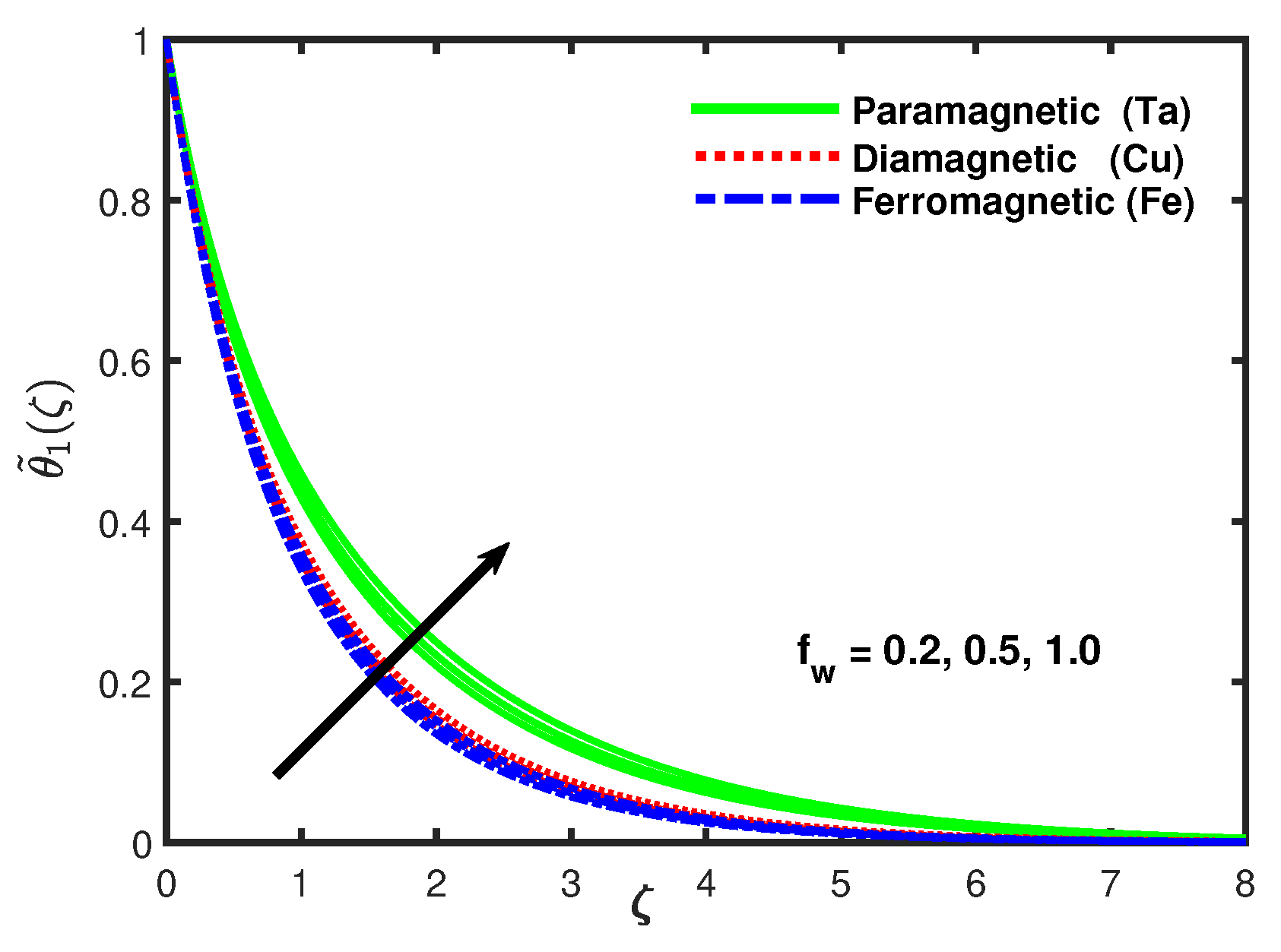
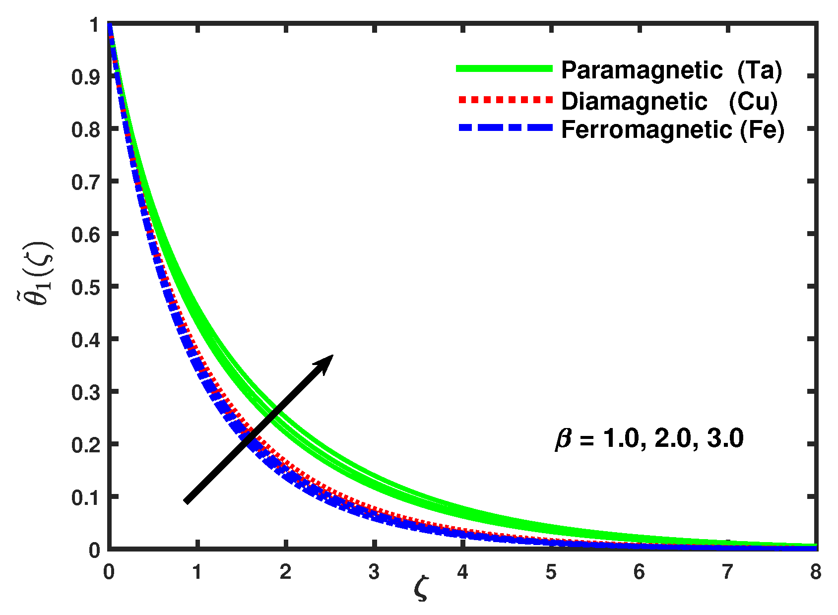
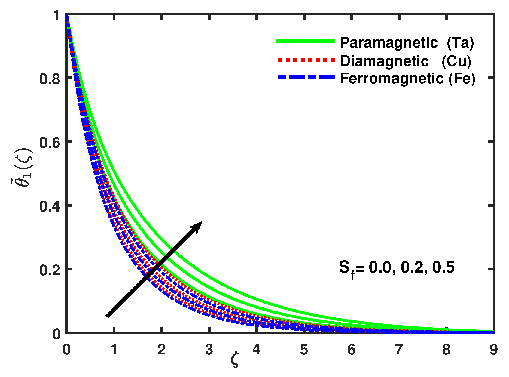
• With increasing values of thermal stratification $S_1$ corresponds in decreasing of velocity and temperature profiles, Further, the heat transfer rate increases by increasing values of parameter $S_1$.
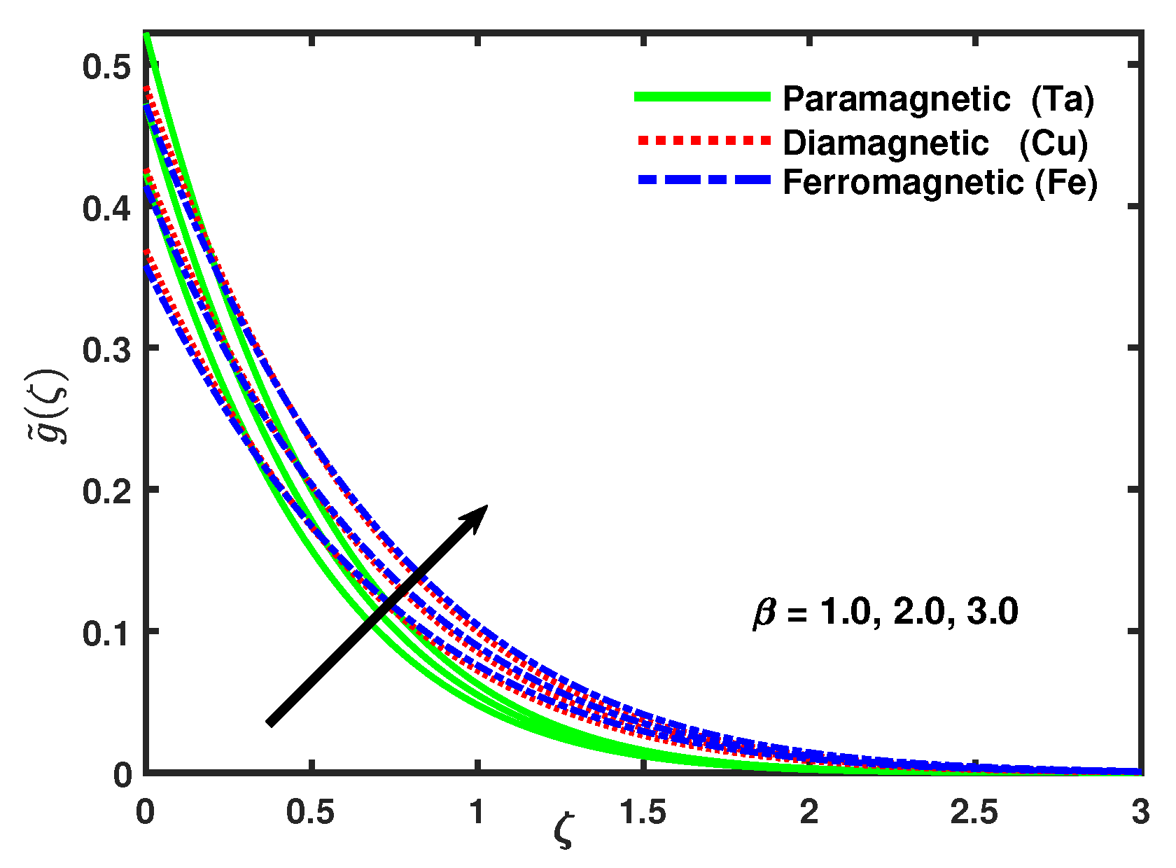
• The velocity, temperature, and micro-rotational velocity is higher in the micropolar ferromagnetic fluid as compare to the ferrimagnetic fluid.
• Thermal conduction of nanoparticles enhances with the inconsistency of volume fraction.
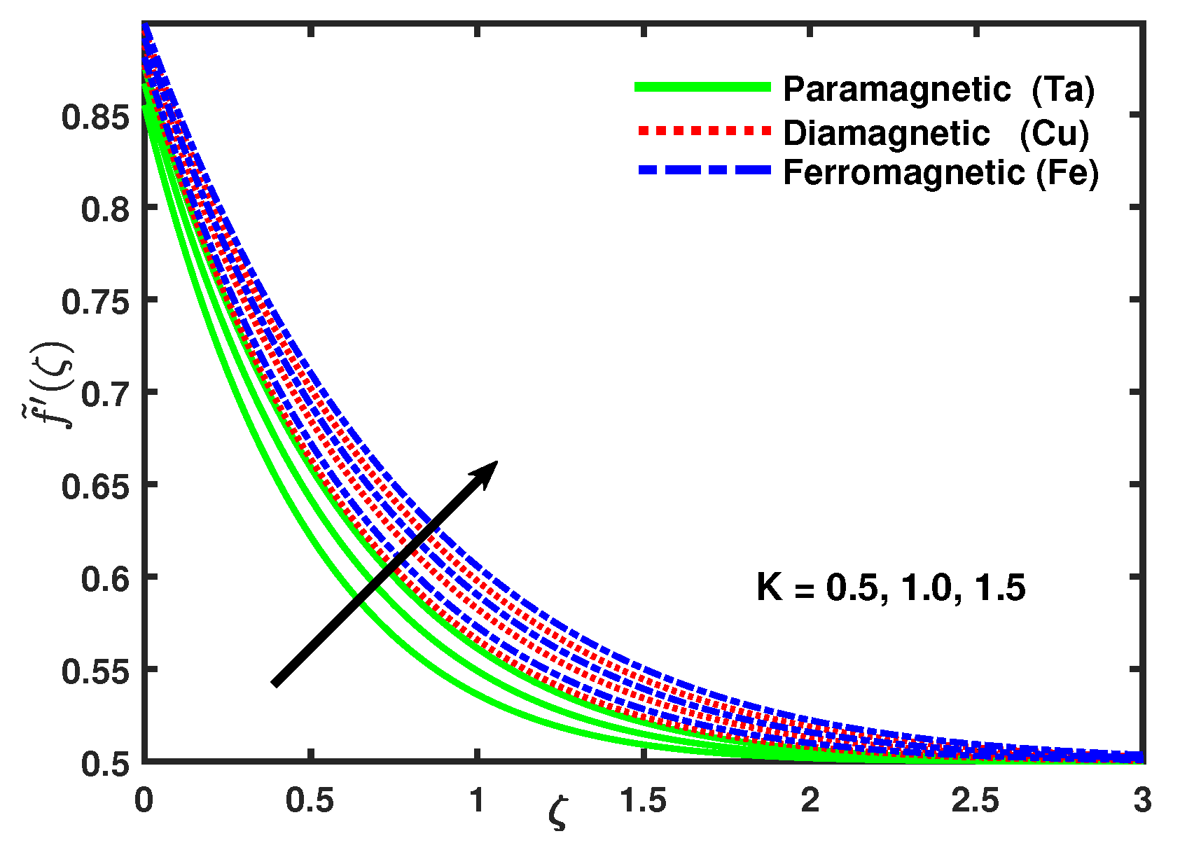
• The effect of K on the velocity profile and the micro-rotational velocity is increasing whereas it is declining in the thermal boundary layer.
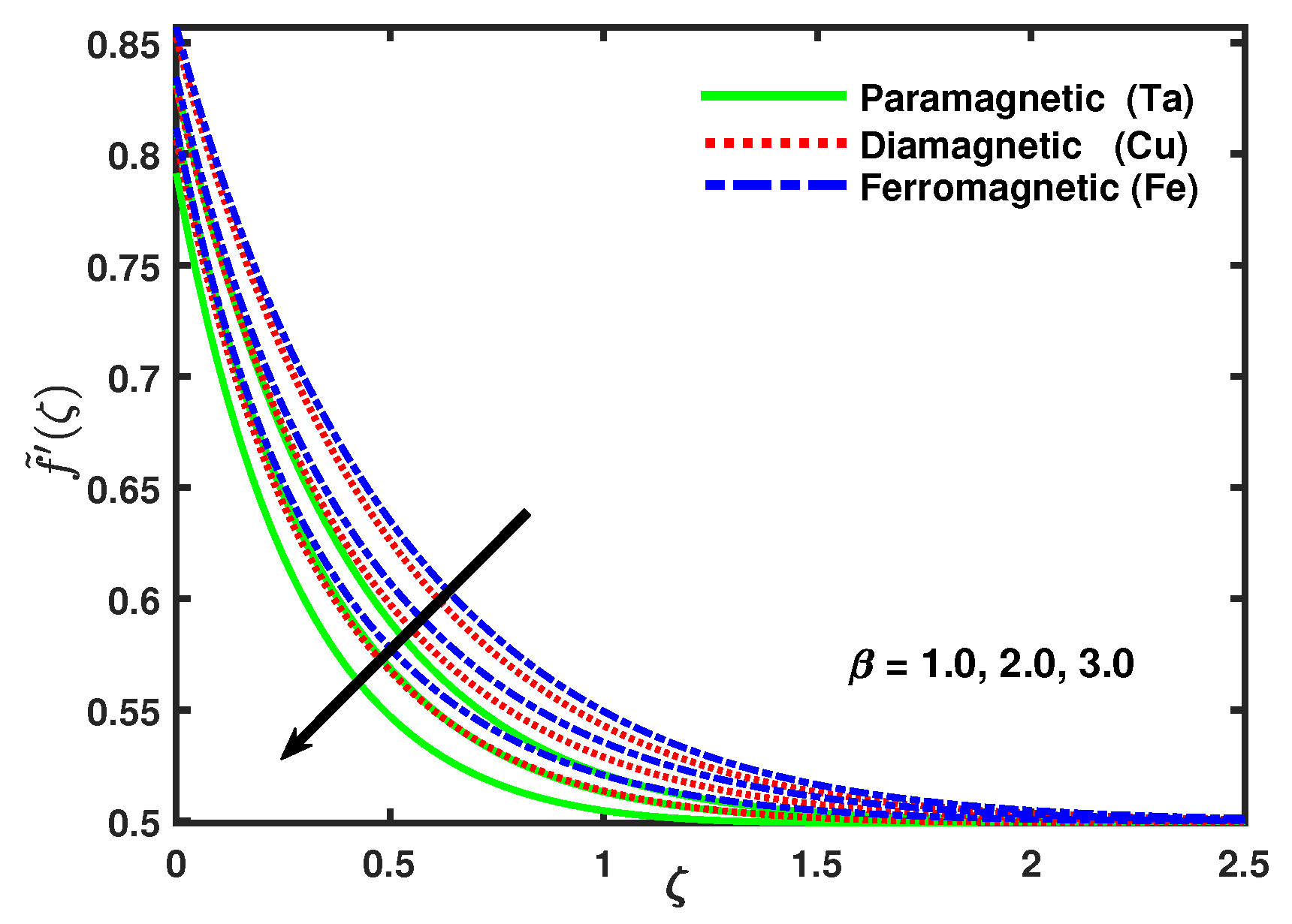
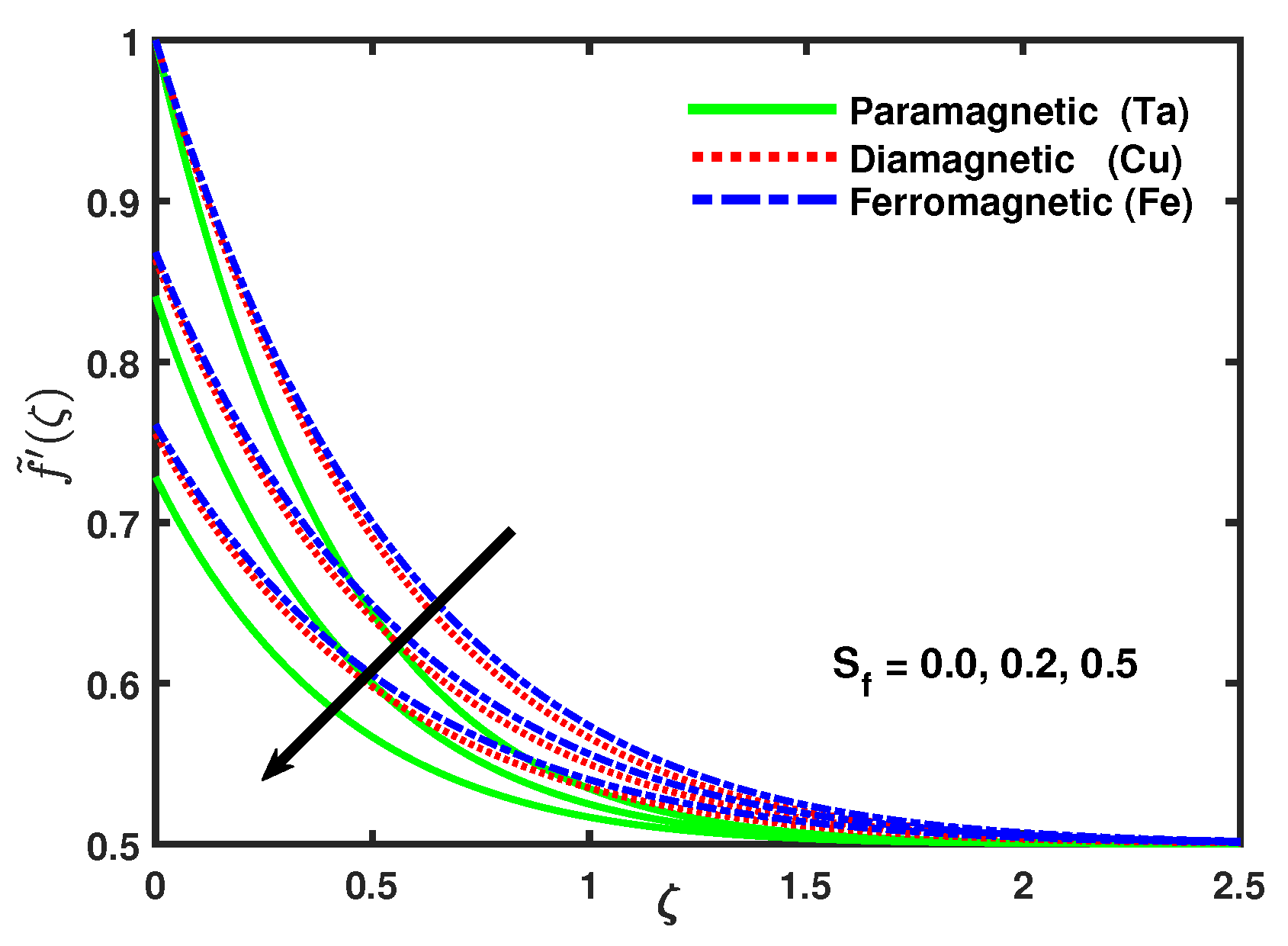
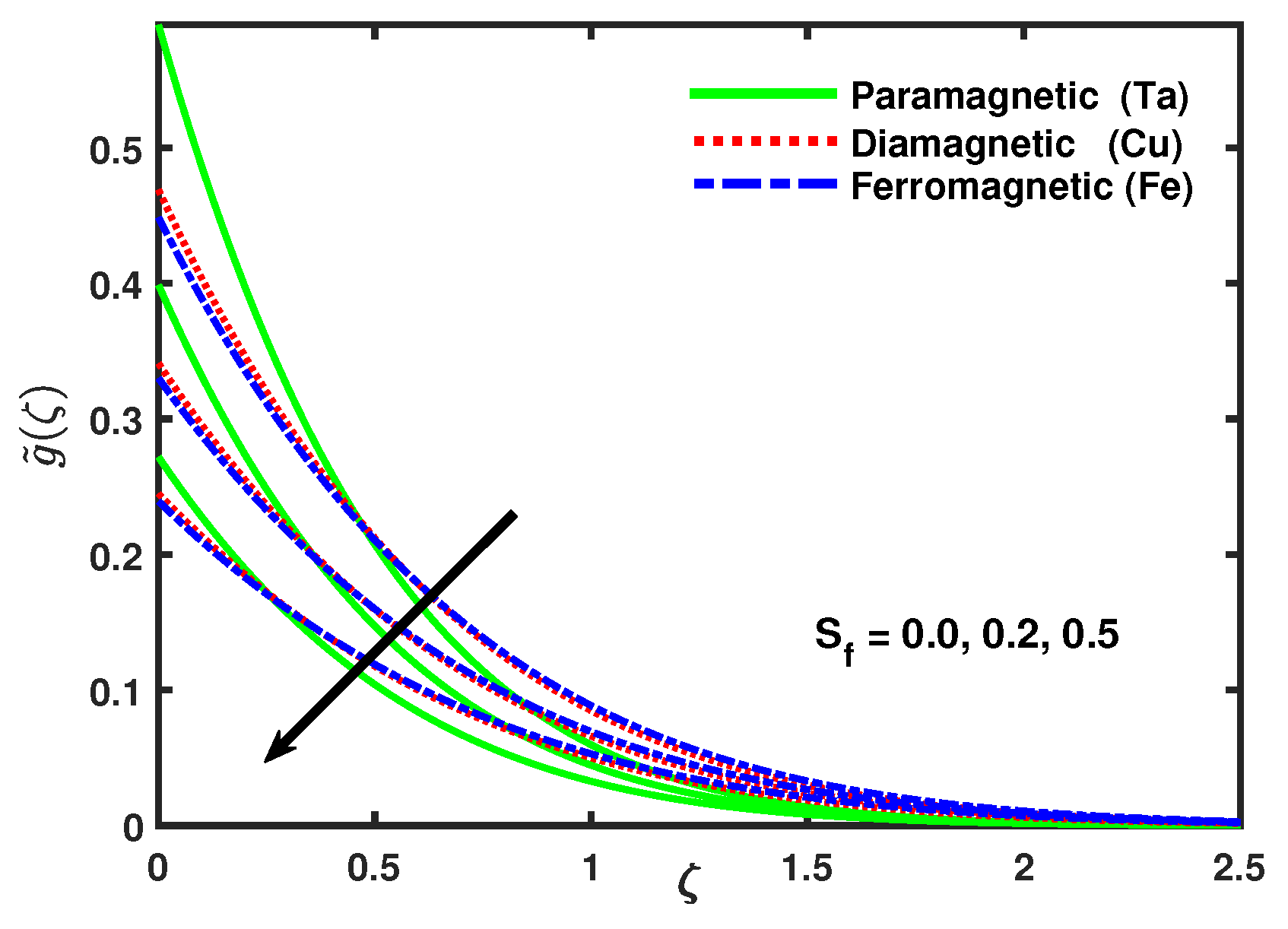
• The velocity profile reduces with increasing values of suction/injection parameter $f_w$ and ferromagnetic parameter $\beta$ in the presence of magnetic dipole while the temperature field increases.
• The velocity profile is a decreasing function of slip parameter $S_f$ while also an increasing function of temperature profile and relative boundary layer of nanofluids.
• In the presence of magnetic dipole reducing the rate of heat transfer has been perceived.

References

1. Esfe, M.H.; Saedodin, S.; Akbari, M.; Karimipour, A.; Afrand, M.; Wongwises, S.; Safaei, M.R.; Dahari, M. Experimental investigation and development of new correlations for thermal conductivity of CuO/EG–water nanofluid. Int. Commun. Heat Mass Transf. 2015, 65, 47–51. [Google Scholar] [CrossRef]
2. Keblinski, P.; Prasher, R.; Eapen, J. Thermal conductance of nanofluids: Is the controversy over? J. Nanoparticle Res. 2008, 10, 1089–1097. [Google Scholar] [CrossRef]
3. Godson, L.; Raja, B.; Lal, D.M.; Wongwises, S. Enhancement of heat transfer using nanofluids—An overview. Renew. Sustain. Energy Rev. 2010, 14, 629–641. [Google Scholar] [CrossRef]
4. Akbar, N.S. Ferromagnetic CNT suspended H2O+Cu nanofluid analysis through composite stenosed arteries with permeable wall. Phys. E Low-Dimens. Syst. Nanostruct. 2015, 72, 70–76. [Google Scholar] [CrossRef]
5. Frey, N.A.; Peng, S.; Cheng, K.; Sun, S. Magnetic nanoparticles: Synthesis, functionalization, and applications in bioimaging and magnetic energy storage. Chem. Soc. Rev. 2009, 38, 2532–2542. [Google Scholar] [CrossRef] [PubMed]
6. Kami, D.; Takeda, S.; Itakura, Y.; Gojo, S.; Watanabe, M.; Toyoda, M. Application of magnetic nanoparticles to gene delivery. Int. J. Mol. Sci. 2011, 12, 3705–3722. [Google Scholar] [CrossRef] [PubMed] [Green Version]
7. Crane, L.J. Flow past a stretching plate. Z. Angew. Math. Phys. ZAMP 1970, 21, 645–647. [Google Scholar] [CrossRef]
8. Sarafraz, M.; Tlili, I.; Tian, Z.; Khan, A.R.; Safaei, M.R. Thermal analysis and thermo-hydraulic characteristics of zirconia–water nanofluid under a convective boiling regime. J. Therm. Anal. Calorim. 2020, 139, 2413–2422. [Google Scholar] [CrossRef]
9. Odenbach, S. Ferrofluids: Magnetically Controllable Fluids and Their Applications; Springer: Berlin/Heidelberg, Germnay, 2008; Volume 594. [Google Scholar]
10. Neuringer, J.L. Some viscous flows of a saturated ferro-fluid under the combined influence of thermal and magnetic field gradients. Int. J. Non-Linear Mech. 1966, 1, 123–137. [Google Scholar] [CrossRef]
11. Sharma, A.; Sharma, D.; Sharma, R. Effect of dust particles on thermal convection in a ferromagnetic fluid. Z. Naturforschung A 2005, 60, 494–502. [Google Scholar]
12. Mee, C. The mechanism of colloid agglomeration in the formation of Bitter patterns. Proc. Phys. Soc. Sect. A 1950, 63, 922. [Google Scholar] [CrossRef]
13. Nadeem, S.; Raishad, I.; Muhammad, N.; Mustafa, M. Mathematical analysis of ferromagnetic fluid embedded in a porous medium. Results Phys. 2017, 7, 2361–2368. [Google Scholar] [CrossRef]
14. Sheikholeslami, M. Numerical simulation of magnetic nanofluid natural convection in porous media. Phys. Lett. A 2017, 381, 494–503. [Google Scholar] [CrossRef]
15. Madhu, M.; Kishan, N. Finite element analysis of heat and mass transfer by MHD mixed convection stagnation-point flow of a non-Newtonian power-law nanofluid towards a stretching surface with radiation. J. Egypt. Math. Soc. 2016, 24, 458–470. [Google Scholar] [CrossRef] [Green Version]
16. Bognár, G.; Hriczó, K. Ferrofluid Flow in the Presence of Magnetic Dipole. Tech. Mech. 2019, 39, 3–15. [Google Scholar]
17. Ali, B.; Yu, X.; Sadiq, M.T.; Rehman, A.U.; Ali, L. A Finite Element Simulation of the Active and Passive Controls of the MHD Effect on an Axisymmetric Nanofluid Flow with Thermo-Diffusion over a Radially Stretched Sheet. Processes 2020, 8, 207. [Google Scholar] [CrossRef] [Green Version]
18. Li, Q.; Xuan, Y.; Wang, J. Experimental investigations on transport properties of magnetic fluids. Exp. Therm. Fluid Sci. 2005, 30, 109–116. [Google Scholar] [CrossRef]
19. Ali, L.; Liu, X.; Ali, B.; Mujeed, S.; Abdal, S.; Khan, S.A. Analysis of Magnetic Properties of Nano-Particles Due to a Magnetic Dipole in Micropolar Fluid Flow over a Stretching Sheet. Coatings 2020, 10, 170. [Google Scholar] [CrossRef] [Green Version]
20. Yirga, Y.; Tesfay, D. Heat and mass transfer in MHD flow of nanofluids through a porous media due to a permeable stretching sheet with viscous dissipation and chemical reaction effects. Int. J. Mech. Aerospace Ind. Mech. Manuf. Eng. 2015, 9, 674–681. [Google Scholar]
21. Nadeem, S.; Muhammad, N. Impact of stratification and Cattaneo-Christov heat flux in the flow saturated with porous medium. J. Mol. Liquids 2016, 224, 423–430. [Google Scholar] [CrossRef]
22. Muhammad, N.; Nadeem, S.; Haq, R.U. Heat transport phenomenon in the ferromagnetic fluid over a stretching sheet with thermal stratification. Results Phys. 2017, 7, 854–861. [Google Scholar] [CrossRef]
23. Ali, L.; Liu, X.; Ali, B.; Mujeed, S.; Abdal, S. Finite Element Simulation of Multi-Slip Effects on Unsteady MHD Bioconvective Micropolar nanofluid Flow Over a Sheet with Solutal and Thermal Convective Boundary Conditions. Coatings 2019, 9, 842. [Google Scholar] [CrossRef]
24. Khan, S.A.; Nie, Y.; Ali, B. Multiple slip effects on MHD unsteady viscoelastic nano-fluid flow over a permeable stretching sheet with radiation using the finite element method. SN Appl. Sci. 2020, 2, 66. [Google Scholar] [CrossRef] [Green Version]
25. Turkyilmazoglu, M. Flow of a micropolar fluid due to a porous stretching sheet and heat transfer. Int. J. Non-Linear Mech. 2016, 83, 59–64. [Google Scholar] [CrossRef]
26. Shadloo, M.; Kimiaeifar, A.; Bagheri, D. Series solution for heat transfer of continuous stretching sheet immersed in a micropolar fluid in the existence of radiation. Int. J. Numer. Methods Heat Fluid Flow 2013, 23, 289–304. [Google Scholar] [CrossRef]
27. Pradhan, S.; Baag, S.; Mishra, S.; Acharya, M. Free convective MHD micropolar fluid flow with thermal radiation and radiation absorption: A numerical study. Heat Transf. Asian Res. 2019, 48, 2613–2628. [Google Scholar] [CrossRef]
28. Bahiraei, M.; Mazaheri, N.; Aliee, F.; Safaei, M.R. Thermo-hydraulic performance of a biological nanofluid containing graphene nanoplatelets within a tube enhanced with rotating twisted tape. Powder Technol. 2019, 355, 278–288. [Google Scholar] [CrossRef]
29. Eringen, A.C. Theory of micropolar fluids. J. Math. Mech. 1966, 16, 1–18. [Google Scholar] [CrossRef]
30. Ahmadi, G. Self-similar solution of imcompressible micropolar boundary layer flow over a semi-infinite plate. Int. J. Eng. Sci. 1976, 14, 639–646. [Google Scholar] [CrossRef]
31. Gorla, R.S.R. Micropolar boundary layer flow at a stagnation point on a moving wall. Int. J. Eng. Sci. 1983, 21, 25–33. [Google Scholar] [CrossRef]
32. Ibrahim, W.; Shankar, B. MHD boundary layer flow and heat transfer of a nanofluid past a permeable stretching sheet with velocity, thermal and solutal slip boundary conditions. Comput. Fluids 2013, 75, 1–10. [Google Scholar] [CrossRef]
33. Das, K. Slip flow and convective heat transfer of nanofluids over a permeable stretching surface. Comput. Fluids 2012, 64, 34–42. [Google Scholar] [CrossRef]
34. Abbas, Z.; Wang, Y.; Hayat, T.; Oberlack, M. Slip effects and heat transfer analysis in a viscous fluid over an oscillatory stretching surface. Int. J. Numer. Methods Fluids 2009, 59, 443–458. [Google Scholar] [CrossRef]
35. Abdal, S.; Ali, B.; Younas, S.; Ali, L.; Mariam, A. Thermo-Diffusion and Multislip Effects on MHD Mixed Convection Unsteady Flow of Micropolar Nanofluid over a Shrinking/Stretching Sheet with Radiation in the Presence of Heat Source. Symmetry 2020, 12, 49. [Google Scholar] [CrossRef] [Green Version]
36. Titus, L.; Abraham, A. Ferromagnetic Liquid Flow due to Gravity-Aligned Stretching of an Elastic Sheet. J. Appl. Fluid Mech. 2015, 8, 591–600. [Google Scholar] [CrossRef]
37. Tiwari, R.K.; Das, M.K. Heat transfer augmentation in a two-sided lid-driven differentially heated square cavity utilizing nanofluids. Int. J. Heat Mass Transf. 2007, 50, 2002–2018. [Google Scholar] [CrossRef]
38. Andersson, H.; Valnes, O. Flow of a heated ferrofluid over a stretching sheet in the presence of a magnetic dipole. Acta Mech. 1998, 128, 39–47. [Google Scholar] [CrossRef]
39. Palaniappan, B.; Ramasamy, V. Thermodynamic analysis of fly ash nanofluid for automobile (heavy vehicle) radiators. J. Therm. Anal. Calorim. 2019, 136, 223–233. [Google Scholar] [CrossRef]
40. Domkundwar, A.; Domkundwar, V. Heat and Mass Transfer Data Book; Dhanpat Rai: New Delhi, India, 2007. [Google Scholar]
41. Ali, B.; Naqvi, R.A.; Nie, Y.; Khan, S.A.; Sadiq, M.T.; Rehman, A.U.; Abdal, S. Variable Viscosity Effects on Unsteady MHD an Axisymmetric Nanofluid Flow over a Stretching Surface with Thermo-Diffusion: FEM Approach. Symmetry 2020, 12, 234. [Google Scholar] [CrossRef] [Green Version]
42. Gupta, D.; Kumar, L.; Bég, O.A.; Singh, B. Finite element analysis of MHD flow of micropolar fluid over a shrinking sheet with a convective surface boundary condition. J. Eng. Thermophys. 2018, 27, 202–220. [Google Scholar] [CrossRef]
43. Bhargava, R.; Rana, P. Finite element solution to mixed convection in MHD flow of micropolar fluid along a moving vertical cylinder with variable conductivity. Int. J. Appl. Math. Mech. 2011, 7, 29–51. [Google Scholar]
44. Khan, S.A.; Nie, Y.; Ali, B. Stratification and Buoyancy Effect of Heat Transportation in Magnetohydrodynamics Micropolar Fluid Flow Passing over a Porous Shrinking Sheet Using the Finite Element Method. J. Nanofluids 2019, 8, 1640–1647. [Google Scholar] [CrossRef]
45. Reddy, J.N. Solutions Manual for an Introduction to the Finite Element Method; McGraw-Hill: New York, NY, USA, 1993; Volume 27, p. 41. [Google Scholar]
46. Swapna, G.; Kumar, L.; Rana, P.; Singh, B. Finite element modeling of a double-diffusive mixed convection flow of a chemically-reacting magneto-micropolar fluid with convective boundary condition. J. Taiwan Inst. Chem. Eng. 2015, 47, 18–27. [Google Scholar] [CrossRef]
47. Gupta, D.; Kumar, L.; Beg, O.A.; Singh, B. Finite-element analysis of transient heat and mass transfer in microstructural boundary layer flow from a porous stretching sheet. Comput. Therm. Sci. Int. J. 2014, 6, 155–169. [Google Scholar] [CrossRef]
48. Ali, L.; Liu, X.; Ali, B.; Mujeed, S.; Abdal, S. Finite Element Analysis of Thermo-Diffusion and Multi-Slip Effects on MHD Unsteady Flow of Casson Nano-Fluid over a Shrinking/Stretching Sheet with Radiation and Heat Source. Appl. Sci. 2019, 9, 5217. [Google Scholar] [CrossRef] [Green Version]
49. Ali, B.; Nie, Y.; Khan, S.A.; Sadiq, M.T.; Tariq, M. Finite Element Simulation of Multiple Slip Effects on MHD Unsteady Maxwell Nanofluid Flow over a Permeable Stretching Sheet with Radiation and Thermo-Diffusion in the Presence of Chemical Reaction. Processes 2019, 7, 628. [Google Scholar] [CrossRef] [Green Version]
50. Majeed, A.; Zeeshan, A.; Ellahi, R. Unsteady ferromagnetic liquid flow and heat transfer analysis over a stretching sheet with the effect of dipole and prescribed heat flux. J. Mol. Liq. 2016, 223, 528–533. [Google Scholar] [CrossRef]
51. Bachok, N.; Ishak, A.; Nazar, R. Flow and heat transfer over an unsteady stretching sheet in a micropolar fluid. Meccanica 2011, 46, 935–942. [Google Scholar] [CrossRef]
52. Qasim, M.; Khan, I.; Shafie, S. Heat transfer in a micropolar fluid over a stretching sheet with Newtonian heating. PLoS ONE 2013, 8, e59393. [Google Scholar] [CrossRef] [Green Version]
53. Hussanan, A.; Salleh, M.Z.; Khan, I. Microstructure and inertial characteristics of a magnetite ferrofluid over a stretching/shrinking sheet using effective thermal conductivity model. J. Mol. Liq. 2018, 255, 64–75. [Google Scholar] [CrossRef]
54. Kumar, L. Finite element analysis of combined heat and mass transfer in hydromagnetic micropolar flow along a stretching sheet. Comput. Mater. Sci. 2009, 46, 841–848. [Google Scholar] [CrossRef]
55. Muhammad, N.; Nadeem, S.; Mustafa, M. Analysis of ferrite nanoparticles in the flow of ferromagnetic nanofluid. PLoS ONE 2018, 13, e0188460. [Google Scholar] [CrossRef] [PubMed] [Green Version]
Figure 1. Configuration of Flow model.
Symmetry 12 00520 g001
Figure 2. Impact of nano-particles and f w on f ˜ ( ζ ) .
Symmetry 12 00520 g002
Figure 3. Impact of nano-particles and f w on g ˜ ( ζ ) .
Symmetry 12 00520 g003
Figure 4. Impact of nano-particles and f w on θ ˜ 1 ( ζ ) .
Symmetry 12 00520 g004
Figure 5. Impact of nano-particles and β on f ˜ ( ζ ) .
Symmetry 12 00520 g005
Figure 6. Impact of nano-particles and β on g ˜ ( ζ ) .
Symmetry 12 00520 g006
Figure 7. Impact of nano-particles and β on θ ˜ 1 ( ζ ) .
Symmetry 12 00520 g007
Figure 8. Impact of nano-particles and K on f ˜ ( ζ ) .
Symmetry 12 00520 g008
Figure 9. Impact of nano-particles and K on g ˜ ( ζ ) .
Symmetry 12 00520 g009
Figure 10. Impact of nano-particles and K on θ ˜ 1 ( ζ ) .
Symmetry 12 00520 g010
Figure 11. Impact of nano-particles and S f on f ˜ ( ζ ) .
Symmetry 12 00520 g011
Figure 12. Impact of nano-particles and S f on g ˜ ( ζ ) .
Symmetry 12 00520 g012
Figure 13. Impact of nano-particles and S f on θ ˜ 1 ( ζ ) .
Symmetry 12 00520 g013
Figure 14. Impact of nano-particles and P r on θ ˜ 1 ( ζ ) .
Symmetry 12 00520 g014
Figure 15. Impact of nano-particles and R d on θ ˜ 1 ( ζ ) .
Symmetry 12 00520 g015
Figure 16. Impact of nano-particles and λ on θ ˜ 1 ( ζ ) .
Symmetry 12 00520 g016
Figure 17. Impact of nano-particles and S 1 on θ ˜ 1 ( ζ ) .
Symmetry 12 00520 g017