Abstract
In the field of engineering, automobile and aerospace components are manufactured based on the desired applications from the metal forming process. For producing better quality of both symmetry and asymmetry mechanical parts, understanding the material deformation and analytical representation of the material ductility behavior for the working material is necessary as the forming procedures carried out mostly in the warm processing conditions. In this work, the hot tensile test flow stress-strain data were utilized to construct the constitutive equation for describing AISI-1045 steel material hot deformation behavior, and the test conditions, such as deformation temperatures and strain rates were 750–950 C and 0.05–1.0 s, respectively. The surface morphology and elemental identification analysis were performed using the field emission scanning electron microscopy (FESEM) coupled with the energy-dispersive X-ray spectroscopy (EDS) mapping setup. In this work, the Arrhenius-type constitutive equation, including the strain compensation, was used to formulate the flow stress prediction model for capturing the material behavior. Besides, the Zener-Hollomon parameter was altered, employing incorporating the effect of strain rate and strain on the flow stress. The empirical model approach was employed to estimate the material model constants from the constitutive equation using the actual test measurements. The population metrics such as coefficient of determination (), sample standard deviation of the error (SSD), standard error of the regression (SER), coefficient of residual variation (CRV), and average absolute relative error (AARE) was employed to confirm the predictability of the proposed models. The computed results are discussed in detail, using numerical and graphical verification’s. From the graphical comparison, the flow stress-strain data achieved from the proposed constitutive model are in good agreement with the actual test measurements. The constitutive model prediction accuracy is found to be improved, like the prediction error range from 3.678% to 2.984%. This evidence proves to be feasible as the newly developed model displayed a significant improvement against the experimental observations.
1. Introduction
AISI-1045 steel is a medium carbon steel material that is extensively used for the automobile industry applications, owing to its mechanical properties. The material properties are such as toughness, wear-resistance, and higher strength for manufacturing camshafts and cams by the forging process. In industrial practice, the processing conditions like alloy content and cooling rate altered for achieving the desirable microstructures and excellent mechanical properties. However, during the metal forming process, metals and alloys undergo an inhomogeneous deformation by cause of hot operating conditions. For this reason, understanding the metals deformation behavior is necessary for determining the working parameters that affect the mechanical properties for providing the well-defined material processing data to the industry [1,2,3,4]. The constitutive equations are often utilized in a form that is suitable to use in finite element (FE) commercial tools. They used to represent the material flow behavior and helps to obtain a better prediction [5,6,7,8]. Moreover, the constitutive equations are categorized as follows: physical, phenomenological, and statistical models [9,10,11,12]. In our previous work [13,14], a detailed discussion on AISI 1045 steel material behavior in hot processing conditionswas carried out using Johnson–Cook (JC), modified JC, and modified Zerilli–Armstrong (ZA) models. The results showed that the modified ZA model was more significant in representing the material deformation behavior compared with the test data than that of others. However, the flow stress model predictability can be improvised by training other available conventional models. For this purpose, in this present investigation, the strain compensated Arrhenius-type constitutive model was adopted to represent the material’s ductility behavior in hot operating conditions.
In the past, there has been information published on constitutive equations to consistently describe the material’s behavior at various loading conditions [15,16,17,18]. Besides, many researchers have discussed the advantage of utilizing the constitutive equations by comparing the outcome of available flow stress models, and they reported that the proposed models could be able to precisely characterize the material behavior because the parameters are determined statistically from the experimental data [19,20,21,22]. Samantaray et al. [23] examined the modified 9Cr-1Mo steel material behavior using the phenomenological models. They stated that the Arrhenius-type constitutive model considering strain compensation can track the material behavior more accurately than the original JC and modified ZA models. The strain effects were incorporated into the constitutive equation to characterize the flow behavior in 42CrMo at elevated temperatures by Lin et al. [24]. They reported that including the strain compensation, the proposed model could predict the material behavior significantly under hot working conditions. Unlike conventional methods, an artificial neural network (ANN) model considering a back-propagation algorithm was adopted by Wu et al. [25] and Xiao et al. [26] to predict the material deformation behavior of two different steel materials. They stated that the trained ANN model found to be more precise in predicting the hot comprehensive behavior than the Arrhenius-type constitutive equations.
However, there are only limited reports on the improvement of the strain compensated Arrhenius-type constitutive model, including strain and strain rate effects, into the Zener-Hollomon (Z) parameter to describe the material behavior accurately. Mandal et al. [27] investigated the problem by incorporating a modified Z parameter into the basic equation for predicting a Ti-modified austenitic stainless steel material flow behavior at high-temperature conditions. A revised constitutive equation was in good correlation with the actual data to predict the flow stress throughout the tested range. Besides, Krishnan et al. [28] reported a valuable outcome for the use of strain-rate compensation in the Z parameter for 9Cr-1Mo ferritic steel. They found that the proposed methodology based on the modified Z parameter provided a better estimation of flow stress for most of the test combinations. Therefore, this present research work aims to establish and devise the suitable constitutive flow stress model over a wide range of testing conditions to describe the AISI-1045 steel material flow behavior. The test conditions, such as deformation temperatures and strain rates are 750–950 C and 0.05–1.0 s, respectively. For this purpose, the real test measurements were used to fit the model equations by both compensations of strain () and strain rate (). Furthermore, the predictability of proposed models was validated against the experimental observations and also discussed statistically by both numerical and graphical validation.
2. Experiments
Isothermal-tension test was carried out to examine the AISI-1045 steel material deformation behavior during hot processing conditions. The chemical compositions (in wt.%) of the work material is summarized in Table 1 [13]. The samples were prepared through a water-jet cutting process according to the ASTM-E8M-subsize standard with 25 gauge length and 3 thickness [13,14]. Experiments were conducted using a computer-controlled servo-hydraulic testing machine, as shown in Figure 1a, at deformation temperatures and strain rates in a range of (750–950 C) and (0.05–1.0 s), respectively [13,14]. To achieve an isothermal environment, the tensile specimen was covered with isolation part, Figure 1b, and in each test condition, three samples tested, Figure 1c, and recorded results were averaged for obtaining true stress-strain (SS) curves. Later, the elastic region was taken out from the SS curves to gain the true plastic region of SS data for the material model parameters estimation [13,14].

Table 1.
Chemical composition of AISI-1045 medium carbon steel (in wt.%) [13].
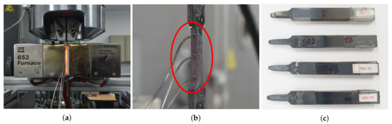
Figure 1.
Elevated temperature tensile testing set-up and procedures (a) Entire test set-up; (b) Test specimen coupled with thermocouples for temperature measurement; (c) Tested specimens.
The typical AISI-1045 medium carbon steel material stress-strain (SS) curves in hot processing conditions are depicted in Figure 2 [13,14,29]. From Figure 2a–c, it is evident that all curves at deformation temperatures 750 C and 950 C exhibit an increment in the flow stress in the initial stage followed by the steady state to strain. Moreover, in Figure 2a–c, deformation temperatures were fixed and flow stress was noticed to be escalated when the strain rate is higher. It happens because if there is an increment in the strain rate, the dislocations and inadequate dynamic recovery and re-crystallization in the material causes the increment in flow stress [13,14]. Similarly, with fixed strain rate (), SS data reduces with increments of the deformation temperature (T) due to the thermal activation energy and the average kinetic energy as it allows the crystals to achieve the dynamic recovery and recrystallization during deformation quickly. Simultaneously, from Figure 2b,c, at strain rates 0.05 s and 0.1 s, the flow stress identified to be decreased dramatically after the small peak stress. This behavior arises due to the plastic instability phenomenon that happened during the tensile test. In detail, when the tensile specimen deformed at a particular stage, there is an unsteadiness between the increase in strength and stress because of work hardening and thinning, respectively [13,14]. At this time, the unstable deformation, decrease in flow stress, appears due to necking and fracture at the test specimen. Thus, this phenomenon has to be considered during the development of empirical based flow stress models.
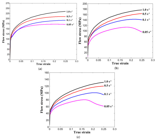
Figure 2.
True stress-strain curves acheived from hot tensile tests at various temperatures (a) 750 C; (b) 850 C; (c) 950 C under different strain rates [13,14,29].
3. Microstructure Evaluation of AISI-1045 Medium Carbon Steel
The field emission scanning electron microscopy (FESEM) and the energy dispersive X-ray spectroscopy (EDS) mapping setups employed to examine the temperature-dependent surface morphology (850 C, 950 C) and elemental identification analysis, respectively, for the tested material [29]. The obtained FESEM micrographs are illustrated in Figure 3. The specimen growth and nucleation is noticed to be uniform on the magnification scale of 50 as displayed in Figure 3a,d in tested temperature conditions. The enlarged portion of 850 C specimen FESEM micrograph, Figure 3b, proves the moderate nanoneedles growth and the micro-fibrils formation at 5 scale [29]. During temperature rise from 850 C to 950 C, the samples were observed to have an apparent growth, nucleation of nanoneedles in the vertical direction along with the micro-fibrils. As a result, it confirms the temperature effect on the tested sample surface, as depicted in Figure 3e. Besides, as shown in Figure 3a,d, the EDS mapping analysis confirms the existence of iron (Fe) and carbon (C) elements all over the examined sample surface ( 100 scale). For proving the thickness reduction in tested samples, at fracture location, the samples scanned at 500 scale as displayed in Figure 3c,f. Moreover, the inset micrographs (Figure 3c,f) illustrate the rough surface morphology of samples at the damaged location ( 5 scale).
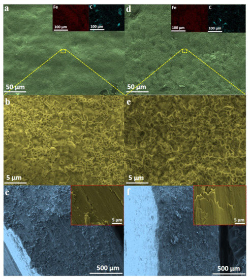
Figure 3.
Field emission scanning electron microscopy (FESEM) and energy dispersive X-ray spectroscopy (EDS) mapping images at strain rate 0.5 s (a–c) 850 C; (d–f) 950 C.
4. Strain Compensated Constitutive Equation for Flow Stress Prediction
4.1. Arrhenius-Type Constitutive Equation
The Arrhenius-type constitutive equations considering the relationship among the strain rate (), flow stress () and deformation temperature (T) has extensively utilized for characterizing the material flow behavior during hot processing conditions. Besides, the Zener-Holloman Z parameter can be used to express the influence of strain rate (), and deformation temperature (T), on the material plastic deformation as follows [5,30]
In Equation (1), the variables, R and Q, are the universal gas constant ( //) and the deformation activation energy, respectively.
At steady-state, the flow stress levels used to select the peak flow stress to estimate values to choose the proper Z equation. There are three levels of Z equation such as the power-law, the exponential, and the hyperbolic sine-law equations as follows [10,30]
where , , , , A, n and are the model constants. is the stress multiplier, . Firstly, by replacing the Z parameter in Equation (2) substituting Equation (1), and then performing the log transformations gives [11,15,30,31]
It is clear that Equations (3)–(5) tend to have a linear relationship form, and the data distributed in Figure 4, Figure 5 and Figure 6 depicts that the correlation exists between the independent variable (x), and the response variable (Y) noticed to be linear. So, the linear regression model is more than enough to capture the variation, and the mathematical form is
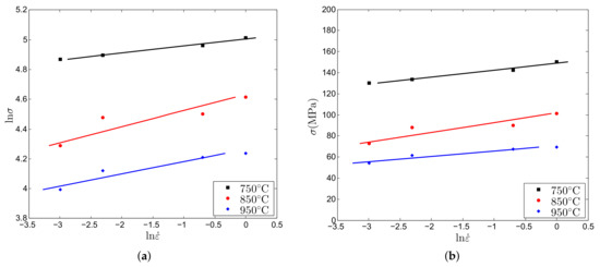
Figure 4.
Relationship plots of and at = 0.02 (a) ln and ln; (b) ln and ; for material constant estimation.
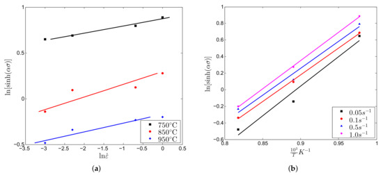
Figure 5.
Relationship plot of and at = 0.02 (a) ln and ln(sinh()); (b) and ln(sinh()); for material constants n and Q estimation.
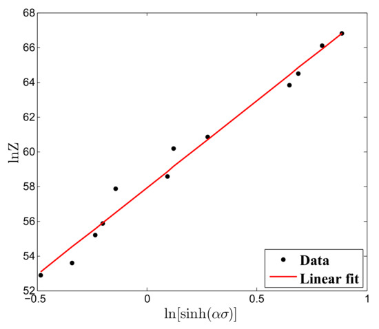
Figure 6.
Correlation plot of stress and strain rate at = 0.02 for material constant estimation.
In Equation (6), , and n are the model intercept, the slope and the number of samples used for the model construction, respectively. Subsequently, the model unknown coefficients are determined using the least squares method as given below
Considering constant deformation temperature, T, from Equations (3)–(5), by taking partial derivatives, the material model constants, , and n, can be estimated as follows [11,30]
In order to estimate the model constants, and n, for example, the stress values associated with the plastic strain value of 0.02, was chosen at tested conditions. By substituting the corresponding values to Equations (3) and (4) and performing the linear regression analysis using Equations (7) and (8), , , and n were determined from the correlation plots of ln and , ln and and ln and ln(sinh()), respectively, as illustrated in Figure 4a,b and Figure 5a. To give a proper understanding of the calculation procedures, the detailed estimation of the model parameter, , at each test conditions and their mean values are listed in Table 2.
Table 2.
Estimation of model parameter, , at strain, = 0.02.
Similarly, considering a specific strain-rate (), by performing a partial derivative of Equation (5), the model parameter, Q, Equation (9), can be estimated as follows [30]
As depicted in Figure 5b, at strain value 0.02, flow stress data at entire deformation temperatures and a specific strain rate were incorporated into Equation (5), and using Equation (7), the material constant, Q, was estimated by averaging four different strain rates outcome from the correlation plot ( and ln(sinh())) and the determined values are summarized in Table 3.
Table 3.
Estimation of model parameters, n and Q, at strain, = 0.02.
For the evaluation of material constant, , Equation (1) is substituted into Equation (2) and performing the log-transform in both sides gives [30,32]
Similarly, considering entire test conditions with their corresponding stress data at plastic strain 0.02 and replacing the model constants in Equations (8) and (10) by estimated values of , n and Q, the material constant, lnA, was determined as 67.4369, from the intercept of Figure 6. In general, the experimental data used to fit Equation (10) to find the material constant, lnA, are summarized in Table 4, and the overall material constants obtained at plastic strain 0.02 are tabulated in Table 5 and by repeating the same procedures, the material constants can be achieved at other selected strain samples.
Table 4.
Estimation of model parameter, lnA, at strain, = 0.02.
Table 5.
Estimated material constants at true plastic strain ( = 0.02).
4.2. Higher Order Polynomial Regression Model
In this section, the mathematical background of regression model is explained in detail to utilize this empirical model in the next section to incorporate the effect of strain on the model constants. A regression function form between the output response and the input variables in terms of any order for estimating the relationship can be expressed as given below [30,34]:
where the column matrix, , is the regression model coefficients. For n number of samples, observed at , Equation (12) can be expressed as follows [30,34]:
In other words, Equation (13) can be simplified and rewritten in matrix notation as
where y, X, and are the response observations, the independent variables, the regression coefficients, and the measurement noises [30,34] in vector and matrix forms. Therefore, the regression coefficients can be determined from the least squares method by performing error minimization between actual and predicted points. The least squares estimate of is [30,34]
Finally, using the estimated , the output response, , for unknown points can be evaluated as follows [30,34]:
4.3. Strain Compensation
From literature survey, many researchers have established the constitutive equations to represent the material flow behaviour of various materials during hot working conditions [6,12,17,28]. However, it is noticed that in Equations (1) and (11), the strain effects are not in consideration and only considered the effects of strain-rate () and deformation temperature (T). Somehow, Lin et al. [35] proved that the strain is having an accountable effect on the flow stress, so the influence of strain should be considered to construct the flow stress model accurately.
In this work, the material constants such as , n, Q, were assessed at selected plastic strains varying from 0.02 to 0.25. The material constants were fitted through order regression function, Equation (12), and the computed model coefficients are tabulated in Table 6; also the systematically estimated material constants curves are sketched as demonstrated in Figure 7 according to selected strain samples using Equations (3)–(5). Moreover, a proposed regression function, Equation (14), was identified to be consistent and adequate to describe the strain effects on the model constants. In addition, the statistical parameters, coefficient of determination () and root mean square error (RMSE), were determined to numerically prove the capability of modeled empirical functions, as illustrated in Figure 7a–d.
Table 6.
Estimated coefficients of fitted empirical models.
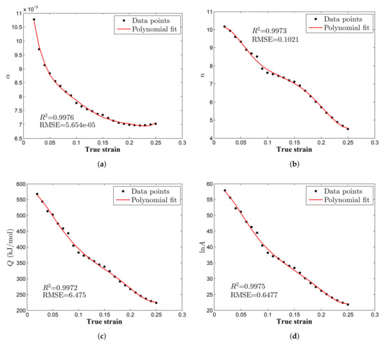
Figure 7.
Material constants correlation plots (a) ; (b) n; (c) Q; (d) ; with true strain.
Here, it is essential to mention that the order of polynomial function can be altered for obtaining a better relationship between the material constants and strains, because the empirical models are only based on the data distribution, not considering any physical performance of the material. Once the materials constants such as Q, , , and n are estimated by considering strain compensation, the flow-stress () at specific strain () can be evaluated as shown below:
Generally, it is significant to examine the proposed statistical model using adjusted and standard error of the regression (SER), Equation (16), rather than standard and sample standard deviation of the error (SSD), Equation (16), parameters. It is typically estimated by considering the number of samples and the number of variables used for constructing the empirical model. Moreover, it is essential to note down that adjusted is always lower than standard and also differs based on the total number of independent variables used for the model construction.
In Equation (16) n and K are the total number of samples and independent variables, respectively. Moreover, the residuals are plotted to discuss about the deviation of prediction data from the actual data in terms of the graphical representation to show the characteristic of prediction errors. As shown in Figure 8a, the residuals appear to be random, but Figure 8b–d, noticed to have a wave patterns, which conveys that the model is missing the interaction terms, however, the prediction error range is identified to be less. Besides, from the numerical verification’s, the range of metrics, SSD, SER and coefficient of residual variation (CRV), are computed as 9.9 × 10 to 104.697, 4.97 × 10 to 5.692 and 0.638% to 1.57%, respectively. These numbers prove that the fitted equations showed a better predictability and Equation (15) can be used further for the material constants computation at unknown plastic strain samples. Using Equation (15), to graphically verify the proposed constitutive equations, the stress-strain curves were developed and compared with experimental observations as depicted in Figure 9a–d. In experimental conditions, 850 C and 950 C for low strain rates, considerable deviations are found among the predicted and the test data as shown in Figure 9a,b. The model constants estimation from the high non-linearity stress data at test temperatures, 850 C and 950 C (low strain rates), due to the plastic instability phenomenon, may caused this moderate variation into flow stress modeling.
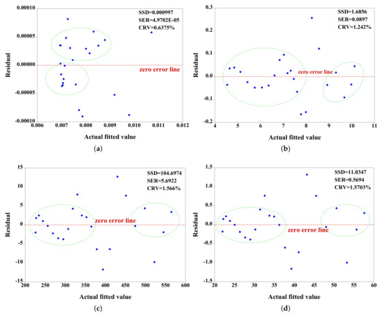
Figure 8.
Residual plot of material constants (a) ; (b) n; (c) Q; (d) .
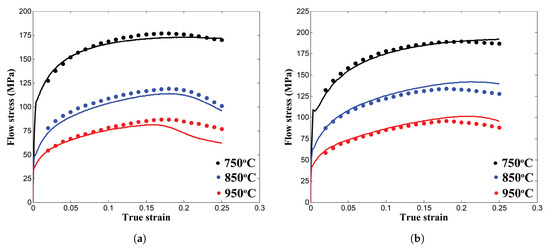
Figure 9.
Stress-strain curves comparison against the predicted curves from the modified constitutive equation (a) 0.05 s; (b) 0.1 s; (c) 0.5 s; (d) 1.0 s.
5. Constitutive Model Verification
Statistical measurements, such as , RMSE, and an average absolute relative error (AARE), are utilized to verify the developed constitutive equations prediction capability at individual strains for en entire test conditions. The first metric— describes how the dependent variables are related to the independent variables in terms of prediction strength; the higher value is better in terms of quality of fit. On the other hand, adjusted explains the model quality based on the number of independent variables used for the model construction. The second metric, RMSE explains the residual locations like how the measured data are diffused to the prediction line; e.g., if RMSE quantity is close to 0, it means the measured data are scattered alongside the regression line or vice versa. The last metric, AARE used to verify the proposed model against the experimental observations considering a term-by-term prediction error [34,36].
where , , are the experimental observations, the predicted stress, and the average stress, respectively. It is most common that adopted to explain the prediction quality of the construted empirical model. However, the higher value of does not necessarily mean that the model has a better fit, it may be due to the number of data points in the selected samples [34,36]. Thus, to confirm the model capability, the graphical validation with systematic comparison was also adopted in this investigation. In this research, to discuss in detail about the prediction strength, an each experimental conditions were examined individually by computing statistical parameters such as and AARE as summarized in Table 7.
Table 7.
Estimated statistical values of the conventional Arrhenius-type constitutive model.
As outlined in Table 7, the computed numerical numbers such as , 0.9817, and AARE, 3.6781%, proves that the proposed constitutive equation is significantly appropriate to represent the material behavior at elevated temperatures; also it is much more suitable for future flow stress prediction at unknown strains. However, from prediction error (AARE), it is identified that there are some difference among the actual test and estimated data in test conditions, 850 C and 950 C (0.05 s and 0.1 s). But somewhat, the disparities are considerably adequate as it shows the significant improvement in the overall metrics as summarized in Table 7. On the other hand, Krishnan et al. [28] and Lin et al. [35] demonstrated that with appropriate modification of the Z parameter considering strain rate compensation, the best prediction for an entire flow stress data can be achieved between flow curves. Thus, the modified parameter with the multiplication factor is [28]
where the material constants , n, Q and lnA can be estimated from the polynomial equations presented in Equation (14). In Equation (22), to find out the best modification parameter, by assuming lower (−) and upper (+) value increments from the middle (0) value, was replaced by considering three different multiplication factors such as , and . Using Equation (23), out of these combinations, was found to have a small prediction error, AARE, as 2.9840%, against experimental data. Table 8 displays that the prediction capability was found to be adequate by strain rate compensation in the constitutive equation. Figure 9a–d and Figure 10a are evident that the developed flow stress equation showed a better resemblance against the actual test data except in the test conditions, 850 C and 950 C at low strain rates. Besides the numerical verification, the graphical methods are developed using the correlation plot, the residual plot, and the histogram plot as depicted in Figure 10b and Figure 11a,b, and Figure 10b is evident that the strong prediction was observed against the measured data. Further, from Figure 11a, it is noted that the data distribution in the residual plot exhibits the random pattern, indicating a good fit for the proposed constitutive model. In detail, as shown in Figure 11a, the error distributions are found to be quite irregular in both positive and negative prediction error regions. Moreover, the residuals exhibit no correlation among them; as a result, the proposed constitutive model can not be improved further by the use of any other additional main or interaction effect terms and on the other hand, the developed constitutive equation is considered to be significant for the flow stress prediction.
Table 8.
Estimated statistical values of the modified Arrhenius-type constitutive model.
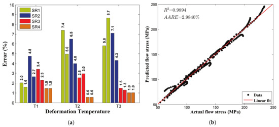
Figure 10.
(a) Bar plot comparison using model errors; (b) Correlation plot between test and computed data.
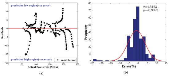
Figure 11.
Graphical validation plots (a) residual plot (at test conditions 750 C and 950 C); (b) Histogram plot.
Besides the residual plot, the error values are plotted to represent the data distribution in a more accurate manner using a histogram plot as illustrated in Figure 11b. Figure 11b is more helpful for understanding about how the residuals are spread out in the space and from Figure 11b, the residuals are identified to fall in a quite acceptable range varies from −8% to 8%. Moreover, from the normal distribution curve, it can be seen that most of the errors fallen inside the range of −5% to 5%, and also the area of probability is not too wide. This graphical evidence suggests that the developed constitutive equation has a significant capability to capture the material ductility behavior at hot operating conditions. Both of the proposed models are displayed an accountable error quantity; because the empirical models do not account the material physical behavior during the excessive deformation and only examine how the data are positioned in the working space. Therefore, a more detailed investigation on the constructed empirical model is required before drawing any reliable conclusions on the proposed constitutive model. However, overall, the estimated prediction error proves that the modified equation provides a better correlation than that of the conventional constitutive equation.
6. Conclusions
The stress-strain (SS) curves of AISI-1045 steel were investigated to describe the material flow behavior under hot working conditions. The test conditions such as deformation temperatures and strain rates are 750–950 C and 0.05–1.0 s, respectively. As well as, the temperature dependent surface morphology, and elemental identification analysis of AISI-1045 steel were carried out using the FESEM and the EDS mapping setup. The Arrhenius-type constitutive equation was developed by considering both influence of strain and strain rate effects on the material constants. A sixth-order regression function was adopted to fit the material constants, and the model adequacies were explained with the help of both numerical and graphical validations. Comparison with experimental results proved that the material flow behavior could be more precisely captured by the modified constitutive equation than the traditional constitutive model. In addition, the conventional constitutive model adequacy was quantified using the statistical parameters and the numerical numbers of and AARE were computed as 0.9817 and 3.6781%, respectively, whereas for the modified constitutive model, the numerical numbers computed as 0.9894 and 2.9840%, respectively. The statistical parameters reflect the significant prediction capability of the proposed strain rate and strain compensated constitutive model. Besides, the newly proposed model can be used in FE tools for performing numerical simulations under hot working conditions.
Author Contributions
In this paper, parts such as experiments, mathematical calculations and the original draft preparation is done by the authors, M.M. and M.S., PhD scholars, and supervision is carried out by D.W.J. All authors have read and agreed to the published version of the manuscript.
Funding
This research received no external funding.
Conflicts of Interest
The authors declare no conflict of interest.
References
- Li, C.; Liu, Y.; Tan, Y.; Zhao, F. Hot Deformation Behavior and Constitutive Modeling of H13-Mod Steel. Metals 2018, 8, 846. [Google Scholar] [CrossRef]
- Li, H.; Jiao, W.; Feng, H.; Li, X.; Jiang, Z.; Li, G.; Wang, L.; Fan, G.; Han, P. Deformation Characteristic and Constitutive Modeling of 2707 Hyper Duplex Stainless Steel under Hot Compression. Metals 2016, 6, 223. [Google Scholar] [CrossRef]
- Liang, Z.; Zhang, Q. Quasi-Static Loading Responses and Constitutive Modeling of Al–Si–Mg alloy. Metals 2018, 8, 838. [Google Scholar] [CrossRef]
- Lei, B.; Chen, G.; Liu, K.; Wang, X.; Jiang, X.; Pan, J.; Shi, Q. Constitutive Analysis on High-Temperature Flow Behavior of 3Cr-1Si-1Ni Ultra-High Strength Steel for Modeling of Flow Stress. Metals 2019, 9, 42. [Google Scholar] [CrossRef]
- Cai, J.; Li, F.; Liu, T.; Chen, B.; He, M. Constitutive equations for elevated temperature flow stress of Ti–6Al–4V alloy considering the effect of strain. Mater. Des. 2011, 32, 1144–1151. [Google Scholar] [CrossRef]
- Slooff, F.A.; Zhou, J.; Duszczyk, J.; Katgerman, L. Constitutive analysis of wrought magnesium alloy Mg–Al4–Zn1. Scr. Mater. 2007, 57, 759–762. [Google Scholar] [CrossRef]
- Ravindranadh, B.; Vemuri, M.; Ashok Kumar, G. Tensile behaviour of aluminium 7017 alloy at various temperatures and strain rates. J. Mater. Res. Technol. 2016, 5, 190–197. [Google Scholar]
- Gan, C.L.; Zheng, K.H.; Qi, W.J.; Wang, M.J. Constitutive equations for high temperature flow stress prediction of 6063 Al alloy considering compensation of strain. Trans. Nonferrous Met. Soc. China 2014, 24, 3486–3491. [Google Scholar] [CrossRef]
- Ma, M.-L.; Li, X.-G.; Li, Y.-J.; He, L.-Q.; Zhang, K.; Wang, X.-W.; Chen, L.-F. Establishment and application of flow stress models of Mg-Y-MM-Zr alloy. Trans. Nonferrous Met. Soc. China. 2011, 21, 857–862. [Google Scholar] [CrossRef]
- Ren, F.-C.; Chen, J. Modeling Flow Stress of 70Cr3Mo Steel Used for Back-Up Roll During Hot Deformation Considering Strain Compensation. J. Iron Steel Res. Int. 2013, 20, 118–124. [Google Scholar] [CrossRef]
- Chai, R.; Guo, C.; Yu, L. Two flowing stress models for hot deformation of XC45 steel at high temperature. Mater. Sci. Eng. A 2012, 534, 101–110. [Google Scholar] [CrossRef]
- Rokni, M.R.; Zarei-Hanzaki, A.; Widener, C.A.; Changizian, P. The Strain-Compensated Constitutive Equation for High Temperature Flow Behavior of an Al-Zn-Mg-Cu Alloy. J. Mater. Eng. Perform. 2014, 23, 4002–4009. [Google Scholar] [CrossRef]
- Murugesan, M.; Jung, D.W. Johnson Cook Material and Failure Model Parameters Estimation of AISI-1045 Medium Carbon Steel for Metal Forming Applications. Materials 2019, 12, 609. [Google Scholar] [CrossRef] [PubMed]
- Murugesan, M.; Jung, D.W. Two flow stress models for describing hot deformation behavior of AISI-1045 medium carbon steel at elevated temperatures. Heliyon 2019, 5, e01347. [Google Scholar] [CrossRef]
- Mirzadeh, H.; Najafizadeh, A. Flow stress prediction at hot working conditions. Mater. Sci. Eng. A 2010, 527, 1160–1164. [Google Scholar] [CrossRef]
- Yang, L.; Pan, Y.; Chen, I.; Lin, D. Constitutive Relationship Modeling and Characterization of Flow Behavior under Hot Working for Fe–Cr–Ni–W–Cu–Co Super-Austenitic Stainless Steel. Metal 2015, 5, 1717–1731. [Google Scholar] [CrossRef]
- Quan, G.; Lv, W.; Mao, Y.; Zhang, Y.; Zhou, J. Prediction of flow stress in a wide temperature range involving phase transformation for as-cast Ti–6Al–2Zr–1Mo–1V alloy by artificial neural network. Mater. Des. 2013, 50, 51–61. [Google Scholar] [CrossRef]
- Sun, M.; Hao, L.; Li, S.; Li, D.; Li, Y. Modeling flow stress constitutive behavior of SA508-3 steel for nuclear reactor pressure vessels. J. Nucl. Mater. 2011, 418, 269–280. [Google Scholar] [CrossRef]
- Abbasi-Bani, A.; Zarei-Hanzaki, A.; Pishbin, M.H.; Haghdadi, N. A comparative study on the capability of Johnson–Cook and Arrhenius-type constitutive equations to describe the flow behavior of Mg–6Al–1Zn alloy. Mech. Mater. 2014, 71, 52–61. [Google Scholar] [CrossRef]
- He, A.; Xie, G.; Zhang, H.; Wang, X. A comparative study on Johnson–Cook, modified Johnson-Cook and Arrhenius-type constitutive models to predict the high temperature flow stress in 20CrMo alloy steel. Mater. Des. 2013, 52, 677–685. [Google Scholar] [CrossRef]
- Han, Y.; Qiao, G.; Sun, J.P.; Zou, D. A comparative study on constitutive relationship of as-cast 904L austenitic stainless steel during hot deformation based on Arrhenius-type and artificial neural network models. Comput. Mater. Sci. 2013, 67, 93–103. [Google Scholar] [CrossRef]
- Senthilkumar, V.; Balaji, A.; Arulkirubakaran, D. Application of constitutive and neural network models for prediction of high temperature flow behavior of Al/Mg based nanocomposite. Trans. Nonferrous Met. Soc. China 2013, 23, 1737–1750. [Google Scholar] [CrossRef]
- Samantaray, D.; Mandal, S.; Bhaduri, A.K. A comparative study on Johnson Cook, modified Zerilli–Armstrong and Arrhenius-type constitutive models to predict elevated temperature flow behaviour in modified 9Cr–1Mo steel. Comput. Mater. Sci. 2009, 47, 568–576. [Google Scholar] [CrossRef]
- Lin, Y.C.; Chen, M.S.; Zhang, J. Modeling of flow stress of 42CrMo steel under hot compression. Mater. Sci. Eng. A 2009, 499, 88–92. [Google Scholar] [CrossRef]
- Wu, R.H.; Liu, J.T.; Chang, H.B.; Hsu, T.Y.; Ruan, X.Y. Prediction of the flow stress of 0.4C–1.9Cr–1.5Mn–1.0Ni–0.2Mo steel during hot deformation. J. Mater. Process. Technol. 2001, 24, 211–218. [Google Scholar] [CrossRef]
- Xiao, X.; Liu, G.Q.; Hu., B.F.; Zheng, X.; Wang, L.N.; Chen, S.J.; Ullah, A. A comparative study on Arrhenius-type constitutive equations and artificial neural network model to predict high-temperature deformation behaviour in 12Cr3WV steel. Comput. Mater. Sci. 2012, 62, 227–234. [Google Scholar] [CrossRef]
- Mandal, S.; Rakesh, V.; Sivaprasad, P.V.; Venugopal, S.; Kasiviswanathan, K.V. Constitutive equations to predict high temperature flow stress in a Ti-modified austenitic stainless steel. Mater. Sci. Eng. A 2009, 500, 114–121. [Google Scholar] [CrossRef]
- Krishnan, S.A.; Phaniraj, C.; Ravishankar, C.; Bhaduri, A.K.; Sivaprasad, P.V. Prediction of high temperature flow stress in 9Cr-1Mo ferritic steel during hot compression. Int. J. Press. Vessels Pip. 2011, 88, 501–506. [Google Scholar] [CrossRef]
- Murugesan, M.; Sajjad, M.; Jung, D.W. Hybrid Machine Learning Optimization Approach to Predict Hot Deformation Behavior of Medium Carbon Steel Material. Metal 2019, 9, 1315. [Google Scholar] [CrossRef]
- Lee, K.; Murugesan, M.; Lee, S.M.; Kang, B.S. A Comparative Study on Arrhenius-Type Constitutive Models with Regression Methods. Trans. Mater. Process. 2017, 26, 18–27. [Google Scholar] [CrossRef]
- Ren, F.Z.; Zhang, J.T.; Gao, Q.R.; Zhu, Y.M.; Su, J.H. Constitutive Equation of Mg-3.5Zn-0.6Y-0.5Zr Alloy under Hot Compression Deformation. Adv. Mater. Res. 2013, 800, 271–275. [Google Scholar] [CrossRef]
- Zhang, Y.; Fan, Q.; Zhang, X.; Zhou, Z.; Xia, Z.; Qian, Z. Avrami Kinetic-Based Constitutive Relationship for Armco-Type Pure Iron in Hot Deformation. Metals 2019, 9, 365. [Google Scholar] [CrossRef]
- Yonghua, D.; Lishi, M.; Huarong, Q.; Runyue, L.; Ping, L. Developed constitutive models, processing maps and microstructural evolution of Pb-Mg-10Al-0.5B alloy. Mater. Charact. 2017, 129, 353–366. [Google Scholar]
- Murugesan, M.; Kang, B.S.; Lee, K. Multi-Objective Design Optimization of Composite Stiffened Panel Using Response Surface Methodology. J. Compos. Res. 2015, 28, 297–310. [Google Scholar] [CrossRef]
- Lin, Y.C.; Chen, M.S.; Zhong, J. Constitutive Modeling for Elevated Temperature Flow Behavior of 42CrMo Steel. Comput. Mater. Sci. 2007, 42, 470–477. [Google Scholar] [CrossRef]
- Rezaei Ashtiani, H.R.; Shahsavari, P. A comparative study on the phenomenological and artificial neural network models to predict hot deformation behavior of AlCuMgPb alloy. J. Alloys Compd. 2016, 687, 263–273. [Google Scholar] [CrossRef]


© 2020 by the authors. Licensee MDPI, Basel, Switzerland. This article is an open access article distributed under the terms and conditions of the Creative Commons Attribution (CC BY) license (http://creativecommons.org/licenses/by/4.0/).