Identification of Apple Tree Leaf Diseases Based on Deep Learning Models

Abstract

Early diagnosis and accurate identification of apple tree leaf diseases (ATLDs) can control the spread of infection, to reduce the use of chemical fertilizers and pesticides, improve the yield and quality of apple, and maintain the healthy development of apple cultivars. In order to improve the detection accuracy and efficiency, an early diagnosis method for ATLDs based on deep convolutional neural network (DCNN) is proposed. We first collect the images of apple tree leaves with and without diseases from both laboratories and cultivation fields, and establish dataset containing five common ATLDs and healthy leaves. The DCNN model proposed in this paper for ATLDs recognition combines DenseNet and Xception, using global average pooling instead of fully connected layers. We extract features by the proposed convolutional neural network then use a support vector machine to classify the apple leaf diseases. Including the proposed DCNN, several DCNNs are trained for ATLDs recognition. The proposed network achieves an overall accuracy of 98.82% in identifying the ATLDs, which is higher than Inception-v3, MobileNet, VGG-16, DenseNet-201, Xception, VGG-INCEP. Moreover, the proposed model has the fastest convergence rate, and a relatively small number of parameters and high robustness compared with the mentioned models. This research indicates that the proposed deep learning model provides a better solution for ATLDs control. It could be also integrated into smart apple cultivation systems.

1. Introduction

Mosaic, Rust, Grey spot, Brown spot, and Alternaria leaf spot are five common apple tree leaf diseases. Early diagnosis and accurate identification of apple tree leaf diseases (ATLDs) can effectively control the spread of infection, reduce losses, and ensure the apple industry’s healthy growth. Traditional plant leaf disease recognition methods mainly rely on expert experiences to manually extract the color, texture, and shape features of disease leaf images [1,2,3]. Due to the complexity and diversity of the captured backgrounds and the disease spots [4], artificially extracted features using image analysis methods are usually limited to specific dataset, when transferred to new dataset, the identification accuracy is not ideal. Furthermore, most of the existing apple disease dataset include images with pure background, dataset with natural cultivation background need to collect to meet the needs of apple disease identification in the environment of natural field.

Deep convolutional neural networks (DCNNs) have good performances in processing two-dimensional data, especially in image and video classification tasks [5]. Lee et al. proposed a convolutional neural network (CNN) system that used plant leaves to automatically identify plants [6]. In 2015, Kawasaki et al. studied the recognition of cucumber foliar diseases based on CNNs, which classified two common cucumber leaf diseases and healthy leaves with an average accuracy of 94.9% [7]. The results showed that the classification features extracted by the CNN-based network model could obtain the best classification performance. In 2016, Sladojevic et al. used deep neural networks to identify 13 common plant diseases. Results showed that their model had an average recognition accuracy of 96.3% [8]. Mohanty et al. used AlexNet and GoogLeNet networks with transfer learning methods to identify 26 diseases of 14 crops in the PlantVillage dataset, and the accuracy on a given test dataset was 99.35% [9]. Ferentinos et al. used a CNN model to identify plant diseases in 2018, from a public dataset with 87,848 images and 58 diseases of 25 species. Their results showed that the highest accuracy could reach 99.53%, and the model could be used as a tool for early warning of plant diseases [10]. Long et al. used AlexNet and GoogLeNet to conduct experiments which compared the learning performance of scratch learning methods and transfer learning methods. They fine-tuned the DCNNs to identify four leaf diseases and healthy leaves of Camellia oleifera. The experimental results showed that the accuracy of DCNN was 96.53%, and transfer learning could accelerate network convergence and improve classification performance [11].

In 2017, Zhang et al. proposed an ATLDs recognition method based on image processing technology and pattern recognition for three types of ATLDs and healthy leaves [12]. Their dataset included 90 images of healthy apple leaves and leaves with white powder, Mosaic, and Rust diseases. The disease identification accuracy of their method was higher than 90%. In 2017, Liu et al. designed a DCNN based on AlexNet for the identification of four ATLDs. The accuracy reached 97.62% on the dataset containing Mosaic, Rust, Brown spot, and Alternaria leaf spot [13]. In 2019, Baranwal. et al. designed a CNN based on LeNet-5 for the identification of three types of ATLDs and healthy leaves. On the dataset with mostly laboratory background containing Black Rot, Rust, Apple Scab, and healthy leaves, the accuracy reached 98.54% [14]. In 2019, Jiang et al. proposed a CNN model named VGG-INCEP for ATLDs including Mosaic, Rust, Grey spot, Brown spot, and Alternaria leaf spot, which achieves the accuracy of 97.14%, and created a real-time fast disease detection model achieving 78.80% mean average accuracy [15]. In 2020, Yong Zhong et al. proposed three loss functions based on the DenseNet-121 deep convolutional network. On the dataset of general Apple Scab, serious Apple Scab, Grey spot, general Rust, serious Rust, and healthy leaves, the accuracy rates are 93.51%, 93.31% and 93.71% for the three loss functions, which are better than the accuracy of cross-entropy loss function [16]. In 2020, Yu et al. proposed a DCNN based on the region of interest to identify ATLDs. A total of 404 images containing Brown spot, Alternaria leaf spot and healthy leaves were identified. On the dataset, the recognition accuracy rate of 84.3% was achieved [17]. In 2020, Albayati et al. proposed a DCNN that combined speeded up robust feature extraction and grasshopper optimization algorithm feature for the identification of three ATLDs and healthy leaves. On the dataset of Black Rot, Rust, Apple Scab, and healthy leaves, the accuracy reached 98.28% [18].

In summary, the DCNN has achieved satisfactory results in cropped disease recognition area. However, the number of ATLD types that can be identified in the existing research is limited, and the accuracy under the real usage scenario needs to be improved.

Aiming at the above problems, this study proposes a DCNN model named Xception Dense Net (XDNet) combining depthwise separable convolution [19] and densely connected structures [20], which applies transfer learning and uses the global average pooling layer instead of the fully connected layer. This paper use XDNet to extract apple leaf disease features, and use a support vector machine (SVM) to classify the diseases. Comparing the classification and recognition performance with other CNNs, the experimental results show that the identification accuracy of the proposed XDNet model is 98.82% on the testing dataset, which is higher than other mentioned CNNs with the same methods of transfer learning and data preprocessing. Moreover, using image augmentation technology and transfer learning increase the accuracy by 7.59%.

The main contributions of this article are summarized as follows:

Firstly, in order to improve the robustness of the model and reduce over-fitting, we collect apple tree diseased leaf images in laboratory and field conditions, in different seasons, at different times of the day, and with different exposure conditions. Besides, we use augmentation techniques of rotation, mirroring, Gaussian noise, salt and pepper noise, adjusting the brightness, sharpness, contrast of images [21], which have enlarged the dataset. The established dataset can well simulate the real shooting environment, image acquisition noise, light changes and transformation changes.

Secondly, inspired by the depthwise separable convolution structure with residual connections used by Xception [19] and the feature reuse characteristic in the dense block of DenseNet [20], this paper proposes a DCNN model to identify ATLDs, which is a combination of depthwise separable convolution and densely connected structure. The depthwise separable convolution structure reduces network parameters, improves training speed, while dense blocks integrate shallow features into deep features better and achieve better feature reuse.

The rest of the work is arranged as follows: Section 2 introduces the collection, division, and preprocessing of ATLDs dataset. Section 3 introduces the basic structure of Xception and DenseNet, and focuses on the proposed XDNet, which is a deep convolutional network model for ATLDs. Section 4 describes the workflow of the ATLDs recognition system and the proposed network performance evaluated through experiments. Finally, Section 5 summarizes the work.

2. Building the Dataset

In order to complete the classification and identification of common ATLDs, firstly, we collect the dataset that can simulate the actual usage scenarios of the system. Then, we complete the dataset preprocessing tasks such as image scaling, dataset expansion, and dataset normalization. Finally, the dataset is divided into three parts for training, validation, and testing.

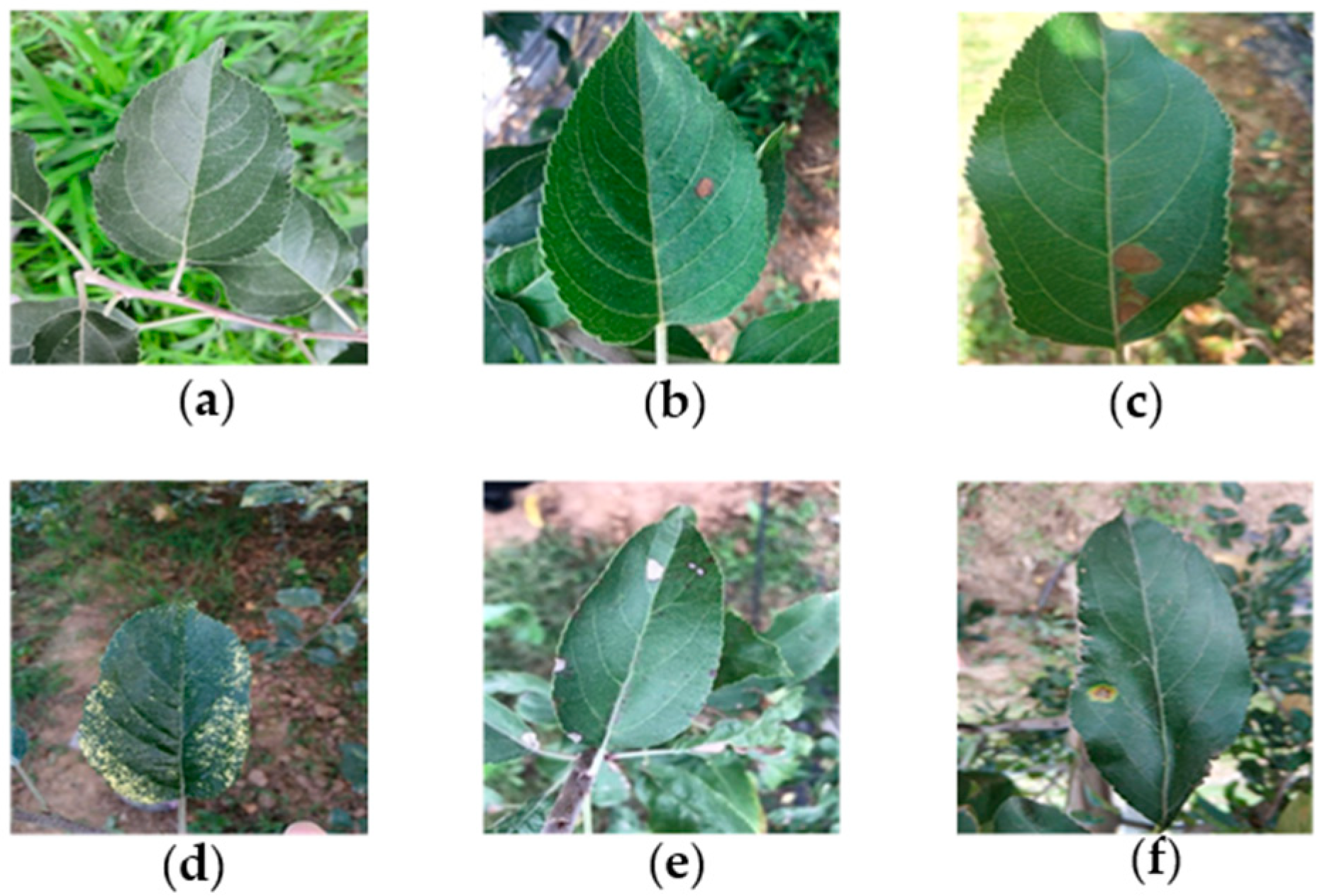
2.1. Collecting the Dataset

Apple tree leaf disease types vary from season, humidity, temperature, light, and other factors. Apple tree leaves may be infected by pathogenic bacteria from tree sprouts to the leaves falling off. In order to fully describe the incidences of the five apple leaf diseases selected and identified in this paper, images of apple leave with different levels of disease were shot in the laboratory (about 38.7%) and real cultivation fields (about 61.3%) with various weather conditions and time periods, which guarantees that the proposed method has higher robustness. A total of 2970 images of ATLDs and healthy leaves were collected. The dataset was evaluated by experts to ensure the validity. The dataset contains five different kinds of diseases and healthy leaves, a total of six types, including Mosaic, Rust, Grey spot, Brown spot, Alternaria leaf spot, and healthy leaves. These five apple leaf diseases are selected because they are frequently noticed in the apple growing area of Shaanxi province, P.R. China, which can cause serious economic losses.

The lesions caused by the same disease show similarity under similar natural conditions. Figure 1 shows the representative images of five common leaf diseases and healthy leaves. It can be seen that five common diseases have obvious distinguishable visual characteristics. The bright yellow spots of Mosaic spread throughout the leaves [22]. The dark brown herpes of Brown spot is morphologically different from other lesions. Near-round yellowish brown lesions are found in the early stage of Grey spot, and then the lesions turn gray subsequently, therefore, the Grey spot in its early stage is easy to be confused with Alternaria leaf spot. The diseased spots of Alternaria leaf spot often have a dark spot or a concentric wheel pattern in the center, which distinguishes them from other lesions. Rust is composed of rusty yellow dots with brown acicular dots in the center of these dots, due to this significant difference, making it easily distinguished from other diseases [15]. Therefore, it is feasible to classify and identify common ATLDs by visual features.

2.2. Dataset Image Preprocessing

Due to powerful end-to-end learning, deep learning models do not require much image preprocessing. We apply data augmentation and data normalization during the preprocessing step.

2.2.1. Data Augmentation

One of the main advantages of CNNs is their ability to generalize, that is, their ability to process data that has never been observed. But when the data size is not large enough and the data diversity is limited, they tend to over-fit the training data, which means they cannot be generalized [23]. In order to enhance the generalization ability of the network and reduce over-fitting, the dataset was expanded by data augmentation technology to simulate changes in lighting, exposure, angle, and noise during the preprocessing step of apple leaf images. In order to simulate these changes, images are processed by increasing and decreasing the brightness value by 30%, increasing the contrast by 50% and decreasing the contrast by 20%, increasing the sharpness by 100% and decreasing the sharpness by 70%, respectively. By using rotation (90°, 180°, 270°), flipping (horizontal and vertical), mirroring, and symmetry operation, the actual shooting angles were simulated. At the same time, in order to simulate the noise that may occur during the image acquisition process, the dataset is further enhanced by adding the interference of appropriate Gaussian noise or salt-and-pepper noise, which can reduce the over-fitting phenomenon in the CNN training stage [2,3,24]. The data augmentation techniques used in this paper are shown in Figure 2. The size of the training dataset has increased by 13 times to 24,976 images after the data augmentation.

2.2.2. Data Normalization

Considering that the deep neural network is very sensitive to the input feature range, a large range of eigenvalues will cause instability during model training [25]. In order to improve the CNN convergence speed and learn subtle differences between images, the dataset is normalized. For each image channels, the data are normalized by Equation (1).

$$Z_i=\frac{x_i-\overline{x}}{{\delta }_x}$$

(1)

where $x_i$, ${\delta }_x$ and $\overline{x}$ are the sample values, channel standard deviation, and channel mean, respectively. By subtracting the mean and dividing by the standard deviation of the channel pixel values, the data have normalized to zero-mean, and all image pixel values are within the range of [−1, 1] [26].

2.3. Dividing the Dataset

For the training and testing of DCNNs, the dataset with 2970 images were divided into three independent subsets, including training dataset, validation dataset, and testing dataset. A total 60% of the dataset composes the training dataset, 20% is used as the validation dataset, and the remaining 20% is used as the testing set, ensuring that each subset contains laboratory background image and natural cultivation background image. The training set is used to train the network, complete the automatic learning of the network, adjust the weights and biases [23]. The validation set is used to adjust the hyper-parameters of the model and perform preliminary evaluation of the model. Lastly, the testing set is used to evaluate the generalization ability of the final model. The aforementioned data augmentation techniques are applied on the training dataset, the validation and testing datasets are not augmented. After performing the above data preprocessing,

Table 1. Number of images for training, validation, and testing.

Disease Types	Original Images	Training Images (After Augmentation)	Validation Images	Testing Images
Alternaria leaf spot	279	2366	55	55
Brown spot	540	4536	108	108
Mosaic	879	7378	176	176
Grey spot	430	3612	86	86
Rust	430	3612	86	86
Heathy	412	3472	82	82
Sum	2970	24,976	593	593

shows the number of images in the training dataset, validation dataset, and testing dataset.

3. Constructing Deep Convolutional Neural Network

CNN started with the original work of LeNet [27] in 1998, then AlexNet [28], ZFNet [29], VGG [30], GoogLeNet [31], ResNet [32], DenseNet [20], Xception [19] etc., appeared. The network is getting deeper, the architecture is becoming more complex, and the method for solving the disappearance of gradients during back propagation is becoming more delicate. Xception uses depthwise separable convolution to separate the spatial convolution and channel convolution operations, and improves the network performance with reduced parameters and calculations. Its residual structure improves gradient dissipation during back-propagation and increases the expression ability of the model. The dense connection structure of DenseNet enhances feature transfer and makes more effective use of features with fewer parameters, but DenseNet consumes a relatively large amount of memory during training. In short, the DenseNet model has good feature reuse capabilities but with large training memory consumption [33]. The depthwise separable convolution of Xception reduces the amount of parameters to a certain extent without reducing model performance. Therefore, this paper proposes the XDNet with a relatively low memory consumption, which keeps the shallow structure of Xception and uses the densely connected structure with feature reuse characteristics in DenseNet replacing the latter part of Xception. The following parts will first introduce the classic Xception and DenseNet models, and then describe thoroughly on how to fuse these two models to get XDNet.

3.1. Xception

Xception [19] is another improvement of Inception-v3 [34] proposed by Google after Inception. The Xception structure is a linear stack of depthwise separable convolutional layers with residual connections. The main features of Xception are as follows:

• The Inception module is replaced by a depthwise separable convolution layer in Xception, and the standard convolution is decomposed into a spatial convolution and a point-by-point convolution. Spatial convolution operations are first performed independently on each channel, followed by point-wise convolution operation, and finally connect the results. The use of depthwise separable convolution can greatly reduce the amount of parameters and calculations with a tiny loss of accuracy. This structure is similar to the conventional convolution operation and can be used to extract features. Compared with the conventional convolution operation, the number of parameters and the calculation cost of depth-wise separable convolution are lower.
• Xception contains 14 modules. Except for the first module and the last module, all modules have added a residual connection mechanism similar to ResNet [32], which significantly accelerates the convergence process of Xception and obtains higher accuracy rate [19]. The structure of Xception network is shown in Figure 3. The front part of the network is mainly used to continuously down sample and reduce the spatial dimension. The middle part is to continuously learn the correlation and optimize the features. The latter part is to summarize and consolidate the features, then Softmax activation function is used to calculate the probability vector of a given input class.

3.2. DenseNet

Compared with VGG, Inception-v3, Xception, and ResNet, DenseNet requires fewer parameters and reasonable calculation time to achieve the best performance [21]. The main characteristics of the DenseNet model are as follows:

• The biggest feature of DenseNet is that for each layer, the function maps of all the previous layers are used as inputs, and its own function map is used as the input of all subsequent layers. It clearly distinguishes the information added to the network from the information reused. The connection scheme is shown in Figure 4, which ensures that the information flow between the layers in the network reaches the maximum, and there is no need to re-learn redundant feature mappings. Therefore, the number of parameters is greatly reduced, and the parameter efficiency is improved. The model improves the information flow and gradient of the entire network. Each layer can directly access the gradient from the loss function to the original input signal, thereby achieving an implicit deep monitoring and alleviating the problem of vanishing gradients. Moreover, the dense connection has regularization effect, so it can restrain the over-fitting on a small scale training dataset to some extent.
• Function maps of the same size between any two layers are directly connected, which has good feed-forward characteristics, enhancing the feature propagation and feature reuse.
• DenseNet has a small number of filters per convolution operation. Only a small part of the feature map is added to the network, and the remaining feature maps are kept unchanged. This structure reduces the number of input feature maps and helps to build a deep network architecture.
• The structure of the DenseNet-201 [20] model is shown in Figure 4. Since the output of the dense block connects all the layers in the block, the larger the depth in the dense block is, the larger the size of the feature map becomes, which will increase the calculation costs continuously. Therefore, the transition layer is added between the dense blocks. The transition layer consists of 1 × 1 convolution and 2 × 2 average-pooling. Through the 2 × 2 average pool, the width and height can be halved to improve the computational efficiency [35].

Due to its feature reuse and hidden depth supervision characteristics, DenseNet can be naturally extended to hundreds of layers, and with the increase of depth and parameters, the accuracy can be improved to a certain degree without over-fitting and performance degradation [20].

3.3. The Proposed XDNet

Xception uses depthwise separable convolutions to reduce model parameters without reducing the model performance. The densely connected dense blocks of DenseNet model increases the model feature reuse capability. If these two characteristics of Xception and DenseNet are combined, it is possible to improve both feature reuse capability and model performance on the basis of a small number of parameters. Therefore, this paper proposes a new DCNN called XDNet for the identification of ATLDs, which integrates Xception and DenseNet. Due to the different levels of abstraction of the data in the multiple convolutional layers of the model, the low-level, middle-level and high-level information are extracted in the shallow, middle, and deep learning frameworks [36]. In general, the first convolutional layer extracts underlying features or small local patterns, such as edges and corners; and the last convolutional layer extracts advanced features, such as image structure. Because the high-level information has a great influence on discriminating leaf disease types [37], a dense connection structure is added to the deep layer of XDNet to improve the feature reuse performance of high-level features. The structure of XDNet is shown in Figure 5a.

The first half of the model uses the structure of a depthwise separable convolution with residual connections, which is the same as in Xception, as shown in Figure 5b,c. To prevent over-fitting, batch normalization is added after each convolutional layer to avoid the problem of gradient disappearance, increase the classification effect, and greatly accelerate the convergence speed [38].

In order to enhance the feature reuse of high-level features and ensure that the information flow among the high-level layers in the network is maximized, we add dense blocks to the latter part of XDNet. As shown in Figure 5d, the dense block transfer features and gradients more efficiently, and increase model recognition effectively. At the same time, in order to effectively alleviate the problems related to over-fitting, the dropout technology is used. In the training process, some neurons are randomly selected with a given probability and discarded in the network when the weights are updated. The dropout technology prevents excessive cooperative adaptation of neurons and helps to form more meaningful independent features [37].

CNNs usually consist of three parts: a convolutional layer, a pooling layer, and a fully connected layer. Convolutional and pooling layers act as feature extractors for the input image, while fully connected layers act as classifiers. The basic purpose of convolution is to automatically extract features from each input image. Compared with traditional feature extractors (SIFT, Gabor, etc.), the strength of CNN lies in its ability to automatically learn the weights and biases of different feature maps, so as to generate powerful feature extractors with specific tasks [39].

The activation function is executed after each convolution. Rectified linear units (ReLU) function [28] is a very popular non-linear activation function that introduces non-linearity into CNN. The ReLU function is defined in Equation (2):

$$\mathrm{f}\left(\mathrm{x}\right)= \max \left(0,\mathrm{x}\right).$$

(2)

In the ReLU layer, each negative value will be removed from the filter image and replaced with 0.

The parameters of XDNet are shown in

Table 2. Related parameters of the XDNet model.

Type	Patch Size/Stride	Output Size
Input	-	224 × 224 × 3
Convolution	3 × 3/2	111 × 111 × 32
Batch Normalization	-	111 × 111 × 32
ReLU	-	111×111 × 32
Convolution	3×3/1	109 × 109 × 64
Batch Normalization	-	109 × 109 × 64
ReLU	-	109 × 109 × 64
Block1 × 3	-	14 × 14 × 728
Block2 × 5	-	14 × 14 × 728
Batch Normalization	-	14 × 14 × 728
ReLU	-	14 × 14 × 728
Block3×6	-	14 × 14 × 800
Batch Normalization	-	14 × 14 × 800
ReLU	-	14 × 14 × 800
Convolution	1 × 1/1	14 × 14 × 400
Pool/Average	2 × 2/2	7 × 7 × 400
Block3 × 12	-	7 × 7 × 544
Batch Normalization	-	7 × 7 × 544
Global Average Pooling	-	544
SVM	-	6

.

In XDNet, the pooling layer after the convolution layer can reduce the dimension of the feature. Each sub-sampling layer reduces the size of the convolution map, and introduces invariability for possible rotation and translation in the input, which generalizes the output of the convolution layer to a higher level. The max-pooling layer and average-pooling layer use the fixed-size sliding window and predefined step size across the feature map. The feature map is compressed to a smaller size by taking the maximum and average values of the filtered feature map, which reduces the computational complexity and control the overfitting to a certain degree [40].

At the end of XDNet, global average pooling is used to replace the full connection without additional model parameters, which can achieve arbitrary image size input. Therefore, the model size and calculation volume are greatly reduced compared to full connection, and over-fitting can be avoided to accelerate network training [39]. The global average pooling layer extracts a 544-dimensional feature vector and directly inputs it into the classification layer, which correlates the high-level features of ATLDs with the classification task directly. A large number of practices have proved that SVM is effective in dealing with small samples, non-linear and high-dimensional pattern recognition and diagnosis [41], and CNNs achieve a small but consistent advantage of replacing the Softmax layer with linear SVM at the top [42]. At the same time, the experiments show that the compared DCNNs have the consistent advantage after using linear SVM instead of Softmax, and the classification accuracy of XDNet with linear one-vs-all SVM on the testing dataset is 0.17% higher than that of Softmax.

Considering that compared with other adaptive learning rate algorithms, the Adam algorithm is easy to implement, has high computing efficiency, requires less memory, has faster convergence speed, and is resistant to the diagonal rescaling of the gradient [43]. Therefore, the Adam algorithm is used to train the neural network in the back propagation to learn the optimal weights and biases, minimize the loss in the neural network. The batch size is set to 16, the epoch is set to 50, and the base learning rate is set to 0.01.

4. Experimental Evaluation

4.1. Experimental Device

XDNet is implemented in Keras deep learning framework based on CNN using python language. The configuration parameters of the experiments are listed in

Table 3. Software and hardware environment.

Configuration Item	Value
CPU	CPU Intel(R) Xeon(R) CPU E5-2620 v4 @ 2.10GHz
GPU	NVIDIA TITAN V 12 GB
RAM	128 GB
Hard Disk	4 TB
Operating System	Ubuntu 16.04.1 LTS (64-bits)

.

4.2. ATLDs Detection Process

ATLDs detection process is shown in Figure 6. Firstly, we collect images of diseased leaves and healthy leaves of apples from both laboratory and orchard fields. The original dataset was classified according to the disease categories by experienced professionals, and the dataset is divided into training, validation, and testing dataset. After that, we perform data augmentation on the training dataset and all images were normalized. Then, the XDNet model proposed in this paper was pre-trained on a subset of PlantVillage dataset, and then the training model was migrated to the ATLDs dataset collected earlier. Finally, the specific disease type of each image in the testing dataset was detected by the model.

4.3. Experimental Results and Analysis

4.3.1. Confusion Matrix

In order to test the generalization performance and stability of the XDNet model, this paper performs the cross-validation five times. A total 20% of the dataset is selected as the testing dataset, and the remaining 80% of the dataset is divided into training dataset and validation dataset with a ratio of 3:1 five times by random permutation, ensuring that the ratio of images with the field background and the laboratory background in each subset is consistent. Five models are obtained through training, and classification accuracies on the test set of these five models are 98.82%, 98.65%, 98.15%, 98.15%, and 97.98%, respectively. The average classification accuracy of the five models is 98.35%, and the standard deviation is 0.363%, these number show that XDNet has good stability. Take the model with accuracy of 98.82% as an example, it is analyzed below.

According to the predicted label of the testing data and the real label, the confusion matrix is made as shown in Figure 7. The rows in the figure represent the original categories, and the columns represent the predicted categories. All correct predictions are on the diagonal cubes. The darker the color of the cube is, the greater the probability it represents. Figure 7 shows that mosaic was 100% recognized by the model. The classification rated of Alternaria leaf spot is 96.36%, which is due to the amount of Alternaria leaf spot images in the training dataset is relatively less. Furthermore, and for the reasons of similar geometric features between Alternaria leaf spot and Grey spot plus the complexity of exposure condition, the model is easily confused in distinguishing Alternaria leaf spot disease from Grey spot disease.

4.3.2. Comparative Experiment of Transfer Learning

The advantages of transfer learning are that it can reduce the number of images required for training, reduce model training costs, shorten training time, alleviate over-fitting and so on [44]. We selected 4213 leaf images of 5 plant species (tomato, cucumber, chili, apple, and grape) from PlantVillage dataset. XDNet was pre-trained on these images, so that a pre-trained model with prior knowledge of crop leaves has been established. The shallow layers of the pre-trained network extract general, low-level features, such as plant leaf edges. These features do not change significantly and are suitable for many data sets and tasks [45]. Therefore, the pre-trained model can be migrated to the ATLDs recognition task. Figure 8 is the comparison of the classification accuracy and convergence rate of the XDNet with and without transfer learning. Acc_1 and loss_1 are the accuracy and loss values of the model running on the validation set with transfer learning, and acc_2 and loss_2 are those without transfer learning. Comparative experiments show that the accuracy of the model with transfer learning is 1.35% higher than the one without transfer learning on the testing dataset. Better convergence is also obtained through transfer learning.

4.3.3. Experiment on Data Augmentation

Data augmentation can help alleviate the problem of over-fitting in CNN’s training stage. In order to diagnose diseases from images collected during the practical use of the model with various brightness, sharpness and contrasts, this paper augmented the training dataset of the original images. By rotating, flipping, adjusting brightness, contrast, sharpness and introducing interference to ensure that the model can learn as many unrelated patterns as possible during the training process [46], thereby, avoiding over-fitting and achieving better performance. Figure 9 is the comparison diagram of the accuracy and the loss of the models trained with and without data augmentation for the training dataset after transfer learning. Acc_1 and loss_1 depicts the accuracy and the loss of the trained model on the validation dataset with data augmentation for the training dataset separately. Acc_2 and loss_2 are the accuracy and loss values of the model on the validation dataset without data enhancement for the training dataset. Comparative experiments show that the accuracy of the model with data augmentation technology is 6.24% higher than the one without data augmentation technology on the testing dataset. As can be seen from Figure 9, the data augmentation technology effectively makes a more stable training process, reduces over-fitting and makes the model more generalized.

4.3.4. Comparison of DCNNs

Figure 10 shows the identification accuracies of XDNet, VGG-INCEP, and five popular CNNs, including MobileNet [47], DenseNet-201, VGG-16 [30], Inception-v3, and Xception. These networks are all pre-trained by the subset of PlantVillage dataset, and then the parameters are transferred to the ATLDs recognition task. Figure 10 shows the classification accuracy and convergence rate of the above seven networks and XDNet on the validation dataset. XDNet has proven to have the highest accuracy and quickest convergence than other models in identifying diseases on the apple leaf dataset.

Table 4. Comparison of training parameters and accuracy of each model.

Model	Input Size	Batch Size	Training Time/min	Parameters	Best Accuracy/%	Average Accuracy/%
Inception-v3	299	16	76.85	21,815,078	97.13	96.59
DenseNet-201	224	16	111.17	18,333,510	98.31	97.50
MobileNet	224	16	30.42	3,235,014	97.47	96.52
VGG-16	224	16	31.72	134,285,126	96.29	95.85
Xception	299	16	133.43	20,873,774	98.48	97.77
VGG-INCEP	224	32	144.27	148,714,950	97.64	97.20
XDNet (Our work)	224	16	86.67	10,159,518	98.82	98.35

compares the seven networks with the training time, the amount of network parameters, the best accuracy and average accuracy of cross-validation on the testing dataset. It is concluded that the calculation time of the VGG-16 model is the least, but the amount of training parameters is comparably large and the accuracy is relatively low. The XDNet model has the highest accuracy. Compared with MobileNet, a lightweight network with the lowest number of parameters and training time, XDNet has slightly more parameters and training time, resulting in a higher accuracy. Both VGG-INCEP and XDNet use the model fusion method, but the number of parameters and calculation time of VGG-INCEP are much higher than XDNet, and the accuracy is lower than XDNet. Compared with the DenseNet and Xception model, XDNet not only has much less training time, but also has a much smaller amount of model parameters. It can be seen that compared with other models, we manage to improve the performance of the XDNet model without increasing the amount of model parameters, while maintain the robustness and the efficiency of the model. As shown in Figure 10, the XDNet model has converged after 16 epochs, and it has the best convergence rate compared to other models. In general, the XDNet model uses relatively less calculation time and fewer parameters to obtain better convergence and achieve highest accuracy of ATLDs identification (98.82%) among the compared seven models.

4.3.5. Importance of Training Images Type

Two CNN models (XDNet and Xception) with better accuracies were further tested on our dataset for the investigation of the importance of training images capturing type. This experiment uses the same data augmentation and transfer learning techniques as Section 2.2.1 and Section 4.3.2. The training, validation and test datasets are divided in the proportion of 6:2:2. Two groups of training and validation datasets were divided, and each group only contains the field background or laboratory background images with the same quantity. In the test dataset, the images with the field background and laboratory background account for 50%, respectively. The experimental results are shown in

Table 5. Models’ accuracy with different training scenarios in respect to images with laboratory background and field background.

Model	Training: Laboratory	Training: Field
	Accuracy	Accuracy
XDNet	76.96%	90.79%
Xception	74.19%	88.62%

. The results show that the accuracies of the models trained by laboratory background images is lower than those trained by field background images (about 14%) on the same test dataset. These show that images captured in the natural growing environment enable these DCNN models better accuracies in the actual using scenarios, and prove the importance of the images captured in actual cultivation conditions for the identification of ATLDs.

4.3.6. Feature Visualization

Feature visualization can better help to understand ATLDs and ease the debugging process of the learning model [37]. Figure 11 is the visualization of the convolution kernels of the different layer. Firstly, as shown in Figure 11b, it can be found that the number of features obtained from the shallow convolution layer is big. The shallow feature data are very close to the original image data, which is similar to the results of edge detection. At this stage, the convolution kernels retain most of the image information, which further verifies the correctness of the transfer learning usage. Secondly, the XDNet model has a strong response to the lesion area, as shown in Figure 11b–d. When we go deeper in the network, fewer descriptive features are obtained, instead, the features become more abstract, and more information about the disease category becomes implicitly available [29]. It also proves that dense block has good feature reuse ability in the deeper layers of the network, using dense blocks helps to improve ATLDs identification ability for XDNet. Moreover, Figure 11e is the shallow layer feature map visualization of diseased images of the other four diseases, and it shows that the XDNet model has a strong response to the lesion area.

5. Conclusions

Applying artificial intelligence to identify ATLDs is helpful to provide ideas for solving the asymmetry of the needs of professional ATLDs identification and the scarcity of expert resources.

Combining the advantages of Xception and DenseNet models, this paper proposes a deep learning network model XDNet with depthwise separable convolutions and densely connected structures for ATLDs recognition. The model can accurately classify five common ATLDs and healthy leaves in the variable shooting conditions, such as different image resolutions, changing lights, contrasts and orientations. The ATLDs dataset we collected contains 2970 images of five common diseases and healthy apple leaves with both laboratory background and complex natural field background. Data augmentation technology and image channel normalization were used to preprocess the dataset, thereby reducing overfitting and enhancing the robustness of the model.

The experiment compared XDNet with Inception-v3, MobileNet, VGG-16, DenseNet-201, Xception, and VGG-INCEP. Among them, XDNet has the highest average accuracy, which is 0.58% higher than that of Xception (the second highest average accuracy) after cross-validation five times on our ATLDs dataset. Moreover, XDNet has the best convergence and relatively few parameters. The experimental results show that the deep convolutional neural network is promising for the classification of leaf diseases.

Model fusion is proven to achieve better results in the paper, which is also a promising direction with great potential for future works. Applying data augmentation techniques and transfer learning can improve model performance and get higher recognition accuracy. The images captured in actual cultivation conditions are important for training models. Therefore, more diverse data can be collected in the future, especially from the natural cultivation environment with different light condition, complex backgrounds, etc., to further improve the model performance. Since the number of model parameters of XDNet is small, the trained model can be integrated into mobile applications to provide farmers the expert-level disease diagnostic services. The applications can also use for dynamic monitoring of leaf diseases in the orchard, and then achieve automatic early disease warning and intelligent pesticide prescription. Except the mobile support by keeping the model light-weighted, we also plan to work on the automatic evaluation of disease severity to provide accurate identification and diagnosis for ATLDs on the mobile devices.

References

1. Mahlein, A.; Rumpf, T.; Welke, P.; Dehne, H.W.; Plumer, L.; Steiner, U.; Oerke, E. Development of spectral indices for detecting and identifying plant diseases. Remote Sens. Environ. 2013, 128, 21–30. [Google Scholar] [CrossRef]
2. Yuan, L.; Huang, Y.; Loraamm, R.W.; Nie, C.; Wang, J.; Zhang, J. Spectral analysis of winter wheat leaves for detection and differentiation of diseases and insects. Field Crop. Res. 2014, 156, 199–207. [Google Scholar] [CrossRef] [Green Version]
3. Qin, F.; Liu, D.; Sun, B.; Ruan, L.; Ma, Z.; Wang, H. Identification of Alfalfa Leaf Diseases Using Image Recognition Technology. PLoS ONE 2016, 11, e0168274. [Google Scholar] [CrossRef] [PubMed] [Green Version]
4. Zhang, S.; Zhang, Q.; LI, P. Apple disease identification based on improved deep convolutional neural network. J. For. Eng. 2019, 4, 107–112. [Google Scholar]
5. Liu, W.; Wang, Z.; Liu, X.; Zeng, N.; Liu, Y.; Alsaadi, F.E. A survey of deep neural network architectures and their applications. Neurocomputing 2017, 234, 11–26. [Google Scholar] [CrossRef]
6. Lee, S.H.; Chan, C.S.; Wilkin, P.; Remagnino, P. Deep-plant: Plant identification with convolutional neural networks. In Proceedings of the 2015 IEEE International Conference on Image Processing (ICIP), Quebec City, QC, Canada, 27–30 September 2015; pp. 452–456. [Google Scholar]
7. Kawasaki, Y.; Uga, H.; Kagiwada, S.; Iyatomi, H. Basic Study of Automated Diagnosis of Viral Plant Diseases Using Convolutional Neural Networks. In Proceedings of the International Symposium on Visual Computing, Las Vegas, NV, USA, 14–16 December 2015; pp. 638–645. [Google Scholar]
8. Sladojevic, S.; Arsenovic, M.; Anderla, A.; Stefanović, D. Deep Neural Networks Based Recognition of Plant Diseases by Leaf Image Classification. Comput. Intell. Neurosci. 2016, 2016, 1–11. [Google Scholar] [CrossRef] [Green Version]
9. Mohanty, S.; Hughes, D.; Salathe, M. Using Deep Learning for Image-Based Plant Disease Detection. Front. Plant Sci. 2016, 7, 1419. [Google Scholar] [CrossRef] [Green Version]
10. Ferentinos, K. Deep learning models for plant disease detection and diagnosis. Comput. Electron. Agric. 2018, 145, 311–318. [Google Scholar] [CrossRef]
11. Long, M.; Ouyang, C.; Liu, H.; Fu, Q. Image recognition of Camellia oleifera diseases based on convolutional neural network & transfer learning. Nongye Gongcheng Xuebao/Trans. Chin. Soc. Agric. Eng. 2018, 34, 194–201. [Google Scholar]
12. Zhang, C.; Zhang, S.; Yang, J.; Shi, Y.; Chen, J. Apple leaf disease identification using genetic algorithm and correlation based feature selection method. Int. J. Agric. Biol. Eng. 2017, 10, 74–83. [Google Scholar]
13. Liu, B.; Zhang, Y.; He, D.; Li, Y. Identification of Apple Leaf Diseases Based on Deep Convolutional Neural Networks. Symmetry 2017, 10, 11. [Google Scholar] [CrossRef] [Green Version]
14. Baranwal, S.; Khandelwal, S.; Arora, A. Deep Learning Convolutional Neural Network for Apple Leaves Disease Detection. In Proceedings of the International Conference on Sustainable Computing in Science, Technology and Management (SUSCOM), Amity University Rajasthan, Jaipur, India, 26–28 February 2019; p. 8. [Google Scholar]
15. Jiang, P.; Chen, Y.; Bin, L.; He, D.; Liang, C. Real-Time Detection of Apple Leaf Diseases Using Deep Learning Approach Based on Improved Convolutional Neural Networks. IEEE Access 2019, 7, 59069–59080. [Google Scholar] [CrossRef]
16. Zhong, Y.; Zhao, M. Research on deep learning in apple leaf disease recognition. Comput. Electron. Agric. 2020, 168, 105146. [Google Scholar] [CrossRef]
17. Yu, H.; Son, C.; Lee, D. Apple Leaf Disease Identification Through Region-of-Interest-Aware Deep Convolutional Neural Network. J. Imaging Sci. Technol. 2020, 64, 20507-1–20507-10. [Google Scholar] [CrossRef] [Green Version]
18. Albayati, J.S.H.; Ustundag, B.B. Evolutionary Feature Optimization for Plant Leaf Disease Detection by Deep Neural Networks. Int. J. Comput. Intell. Syst. 2020, 13, 12–23. [Google Scholar] [CrossRef] [Green Version]
19. Chollet, F. Xception: Deep Learning with Depthwise Separable Convolutions. In Proceedings of the 2017 IEEE Conference on Computer Vision and Pattern Recognition (CVPR), Honolulu, HI, USA, 21–26 July 2017; pp. 1800–1807. [Google Scholar]
20. Huang, G.; Liu, Z.; Der Maaten, L.V.; Weinberger, K.Q. Densely Connected Convolutional Networks. In Proceedings of the 2017 IEEE Conference on Computer Vision and Pattern Recognition (CVPR), Honolulu, HI, USA, 21–26 July 2017; pp. 2261–2269. [Google Scholar]
21. Wang, D.; Chai, X. Application of machine learning in plant diseases recognition. J. Chin. Agric. Mech. 2019, 40, 171–180. [Google Scholar] [CrossRef]
22. Sweet, J.B.; Barbara, D.J. A yellow mosaic disease of horse chestnut (Aesculus spp.) caused by apple mosaic virus. Ann. Appl. Biol. 2008, 92, 335–341. [Google Scholar] [CrossRef]
23. Boulent, J.; Foucher, S.; Théau, J.; St-Charles, P.-L. Convolutional Neural Networks for the Automatic Identification of Plant Diseases. Front. Plant Sci. 2019, 10, 941. [Google Scholar] [CrossRef] [Green Version]
24. Dutot, M.; Nelson, L.M.; Tyson, R.C. Predicting the spread of postharvest disease in stored fruit, with application to apples. Postharvest Biol. Technol. 2013, 85, 45–56. [Google Scholar] [CrossRef]
25. Joharestani, M.; Cao, C.; Ni, X.; Bashir, B.; Talebiesfandarani, S. PM2.5 Prediction Based on Random Forest, XGBoost, and Deep Learning Using Multisource Remote Sensing Data. Atmosphere 2019, 10, 373. [Google Scholar] [CrossRef] [Green Version]
26. Nagasubramanian, K.; Jones, S.; Singh, A.K.; Sarkar, S.; Singh, A.; Ganapathysubramanian, B. Plant disease identification using explainable 3D deep learning on hyperspectral images. Plant Methods 2019, 15, 98. [Google Scholar] [CrossRef] [PubMed]
27. Lecun, Y.; Bottou, L.; Bengio, Y.; Haffner, P. Gradient-Based Learning Applied to Document Recognition. Proc. IEEE 1998, 86, 2278–2324. [Google Scholar] [CrossRef] [Green Version]
28. Krizhevsky, A.; Sutskever, I.; Hinton, G. ImageNet Classification with Deep Convolutional Neural Networks. Neural Inf. Process. Syst. 2012, 25, 1097–1105. [Google Scholar] [CrossRef]
29. Zeiler, M.D.; Fergus, R. Visualizing and Understanding Convolutional Networks. In Proceedings of the European Conference on Computer Vision, Zurich, Switzerland, 6–12 September 2014; pp. 818–833. [Google Scholar]
30. Simonyan, K.; Zisserman, A. Very Deep Convolutional Networks for Large-Scale Image Recognition. In Proceedings of the Computer Vision and Pattern Recognition, Zurich, Switzerland, 6–12 September 2014. [Google Scholar]
31. Szegedy, C.; Liu, W.; Jia, Y.; Sermanet, P.; Reed, S.; Anguelov, D.; Erhan, D.; Vanhoucke, V.; Rabinovich, A. Going deeper with convolutions. In Proceedings of the 2015 IEEE Conference on Computer Vision and Pattern Recognition (CVPR), Boston, MA, USA, 7–12 June 2015; pp. 1–9. [Google Scholar]
32. He, K.; Zhang, X.; Ren, S.; Sun, J. Deep Residual Learning for Image Recognition. In Proceedings of the 2016 IEEE Conference on Computer Vision and Pattern Recognition (CVPR), Las Vegas, NV, USA, 27–30 June 2016; pp. 770–778. [Google Scholar]
33. Pleiss, G.; Chen, D.; Huang, G.; Li, T.; van der Maaten, L.; Weinberger, K. Memory-Efficient Implementation of DenseNets. arXiv 2017, arXiv:1707.06990. [Google Scholar]
34. Szegedy, C.; Vanhoucke, V.; Ioffe, S.; Shlens, J.; Wojna, Z.B. Rethinking the Inception Architecture for Computer Vision. In Proceedings of the 2016 IEEE Conference on Computer Vision and Pattern Recognition (CVPR), Las Vegas, NV, USA, 27–30 June 2016; pp. 2818–2826. [Google Scholar]
35. Song, J.; Kim, W.; Park, K. Finger-vein Recognition Based on Deep DenseNet Using Composite Image. IEEE Access 2019, 7, 66845–66863. [Google Scholar] [CrossRef]
36. Nogueira, K.; Penatti, O.; dos Santos, J. Towards Better Exploiting Convolutional Neural Networks for Remote Sensing Scene Classification. Pattern Recognit. 2017, 61, 539–556. [Google Scholar] [CrossRef] [Green Version]
37. Mahdianpari, M.; Salehi, B.; Rezaee, M.; Mohammadimanesh, F.; Zhang, Y. Very Deep Convolutional Neural Networks for Complex Land Cover Mapping Using Multispectral Remote Sensing Imagery. Remote Sens. 2018, 10, 1119. [Google Scholar] [CrossRef] [Green Version]
38. Ioffe, S.; Szegedy, C. Batch Normalization: Accelerating Deep Network Training by Reducing Internal Covariate Shift. arXiv 2015, arXiv:1502.03167. [Google Scholar]
39. Amara, J.; Bouaziz, B.; Algergawy, A. A Deep Learning-based Approach for Banana Leaf Diseases Classification. In Proceedings of the BTW Workshop, Stuttgart, Germany, 6–10 March 2017; pp. 79–88. [Google Scholar]
40. Hasan, M.; Tanawala, B.; Patel, K. Deep Learning Precision Farming: Tomato Leaf Disease Detection by Transfer Learning. SSRN Electron. J. 2019. [Google Scholar] [CrossRef]
41. Vioix, J.; Douzals, J.P.; Truchetet, F. Development of a Spatial Method for Weed Detection and Localization. In Proceedings of the International Conference on Robotics and Automation, New Orleans, LA, USA, 26 April–1 May 2004; pp. 169–178. [Google Scholar]
42. Tang, Y. Deep Learning using Linear Support Vector Machines. arXiv 2013, arXiv:1306.0239. [Google Scholar]
43. Kingma, D.; Ba, J. Adam: A Method for Stochastic Optimization. In Proceedings of the International Conference on Learning Representations (ICLR), San Diego, CA, USA, 7–9 May 2015; p. 13. [Google Scholar]
44. Dyson, J.; Mancini, A.; Frontoni, E.; Zingaretti, P. Deep Learning for Soil and Crop Segmentation from Remotely Sensed Data. Remote Sens. 2019, 11, 1859. [Google Scholar] [CrossRef] [Green Version]
45. Yosinski, J.; Clune, J.; Bengio, Y.; Lipson, H. How transferable are features in deep neural networks. In Proceedings of the 27th International Conference on Neural Information Processing Systems, Montreal, QC, Canada, 8–13 December 2014; pp. 3320–3328. [Google Scholar]
46. Wang, Y.; Shi, D.; Li, Y.; Cai, S. Studies on identification of microscopic images of chinese Chinese medicinal materials powder based on squeezenet deep network. J. Chin. Electron Microsc. Soc. 2019, 38, 130–138. [Google Scholar]
47. Howard, A.; Zhu, M.; Chen, B.; Kalenichenko, D.; Wang, W.; Weyand, T.; Andreetto, M.; Adam, H. MobileNets: Efficient Convolutional Neural Networks for Mobile Vision Applications. arXiv 2017, arXiv:1704.04861. [Google Scholar]
Figure 1. Healthy apple leaves and five common disease types: (a) healthy leaves; (b) Alternaria leaf spot; (c) Brown spot; (d) Mosaic; (e) Grey spot; and (f) Rust.
Symmetry 12 01065 g001
Figure 2. Example of dataset augmentation: (a) original image; (b) horizontal mirror symmetry; (c) vertical mirror symmetry; (d) rotate 90° clockwise; (e) rotate 180° clockwise; (f) rotate 270° clockwise; (g) high brightness; (h) low brightness; (i) high contrast; (j) low contrast; (k) high sharpness; (l) low sharpness; (m) Gaussian noise; and (n) salt-and-pepper noise.
Symmetry 12 01065 g002
Figure 3. Schematic diagram of the Xception model.
Symmetry 12 01065 g003
Figure 4. Schematic diagram of DenseNet-201 model.
Symmetry 12 01065 g004
Figure 5. XDNet model structure and three types of add block: (a) schematic diagram of XDNet model; (b) Block1; (c) Block2; and (d) Dense Block.
Symmetry 12 01065 g005
Figure 6. Disease detection process.
Symmetry 12 01065 g006
Figure 7. Confusion matrix.
Symmetry 12 01065 g007
Figure 8. Comparison of the accuracy and loss of the networks with and without transfer learning.
Symmetry 12 01065 g008
Figure 9. The comparison of accuracies and losses by epochs between using original dataset and augmented dataset.
Symmetry 12 01065 g009
Figure 10. Classification accuracies of deep convolutional neural networks (DCNNs) and XDNet for the apple tree leaf diseases (ATLDs) task. X axis is the training epoch and Y axis is the classification accuracy of the corresponding network on the validation dataset.
Symmetry 12 01065 g010
Figure 11. Visualization of original disease leaves and features: (a) original image; (b) shallow layer feature map visualization; (c) middle layer feature map visualization; (d) deep layer feature map visualization; and (e) shallow layer feature map visualization of diseased images of the other four diseases.
Symmetry 12 01065 g011