Group Analysis of the Boundary Layer Equations in the Models of Polymer Solutions

Abstract

The famous Toms effect (1948) consists of a substantial increase of the critical Reynolds number when a small amount of soluble polymer is introduced into water. The most noticeable influence of polymer additives is manifested in the boundary layer near solid surfaces. The task includes the ratio of two characteristic length scales, one of which is the Prandtl scale, and the other is defined as the square root of the normalized coefficient of relaxation viscosity (Frolovskaya and Pukhnachev, 2018) and does not depend on the characteristics of the motion. In the limit case, when the ratio of these two scales tends to zero, the equations of the boundary layer are exactly integrated. One of the goals of the present paper is group analysis of the boundary layer equations in two mathematical models of the flow of aqueous polymer solutions: the second grade fluid (Rivlin and Ericksen, 1955) and the Pavlovskii model (1971). The equations of the plane non-stationary boundary layer in the Pavlovskii model are studied in more details. The equations contain an arbitrary function depending on the longitudinal coordinate and time. This function sets the pressure gradient of the external flow. The problem of group classification with respect to this function is analyzed. All functions for which there is an extension of the kernels of admitted Lie groups are found. Among the invariant solutions of the new model of the boundary layer, a special place is taken by the solution of the stationary problem of flow around a rectilinear plate.

1. Introduction

The famous Toms effect [1] consists of a substantial increase of the critical Reynolds number when a small amount of soluble polymer is introduced into liquid. The study of this phenomenon is the subject of many experimental investigations [2,3,4,5,6,7,8,9]. A detailed bibliography of the studies devoted to the flow of polymer solutions in pipes is presented in Reference [10].

For a theoretical description of the dynamics of polymer solutions, the Pavlovskii model [11] and the second-order Rivlin-Ericksen fluid model [12] are commonly used. In both models, the unknown functions are the velocity vector $\mathbf{v}$ and the pressure p. Pavlovskii’s equations have the form

$$\frac{d\mathbf{v}}{dt}=-\frac{1}{\rho }\nabla p+\nu \Delta \mathbf{v}+\kappa \frac{d\Delta \mathbf{v}}{dt},div\mathbf{v}=0,$$

(1)

where, $\frac{d}{dt}=\frac{\partial }{\partial t}+\mathbf{v}·\nabla ,$ $\rho$ is the fluid density, $\nu$ is the kinematic viscosity and $\kappa$ is the normalized relaxation viscosity [13]. These variables are considered positive constants. In the Rivlin-Ericksen model, Equation (1) are replaced by the following:

$$\frac{d\mathbf{v}}{dt}=-\frac{1}{\rho }\nabla p+\nu \Delta \mathbf{v}+\kappa \left(\frac{d\Delta \mathbf{v}}{dt}+2Div(D·W-W·D)\right),div\mathbf{v}=0,$$

(2)

where D and W are the symmetric and antisymmetric parts of the tensor $\nabla \mathbf{v}$, respectively.

The well-posedness of the initial-boundary value problems for systems (1) and (2) was studied in References [14,15,16,17,18,19]. while the group properties of Equations (1) and (2) and the construction of their exact solutions were studied in References [13,20,21,22].

One more model of the motion of aqueous polymer solutions was formulated in Reference [23]. In this model, the relations between the stress tensor and the strain rate tensor contains an integral operator of Volterra type.

The main objective of the present research is to construct boundary layer equations of two mathematical models of the flow of aqueous polymer solutions [11,12]. Another goal is to demonstrate their solutions.

The manuscript is organized as follows. The next section is devoted to deriving boundary layer equations: the equations of the laminar boundary layer in the Pavlovskii and Rivlin-Ericksen models. Section 3 presents the application of the group analysis method for constructing exact solutions of the boundary layer equations corresponding to the Pavlovskii model. In the Section following it, one class of solutions of this system is analyzed. As the admitted Lie group of the studied equations is infinite, then it is useful to apply group foliation, which is presented in Section 5. The stationary equations are considered in Section 6. Section 7 is devoted to the group analysis of the boundary layer equations of the Rivlin-Eriksen fluids. In the Section next to it, three new problems were formulated. The final Section gives concluding remarks.

2. Derivation of Boundary Layer Equations

Most of the publications on the effect of polymer additives on the nature of the movement are associated with a decrease in resistance in the turbulent flow regime in pipes and the boundary layer. Therefore, it is not surprising that it was the turbulent boundary layer that has been the focus of attention of researchers. As for the laminar boundary layer in an aqueous polymer solution, publications on this subject are unknown to us. The equations of the laminar boundary layer in the Pavlovskii and Rivlin-Ericksen models are thus derived below. We restrict ourselves to the case of plane movements.

In coordinate representation, Equation (1) have the form:

$$\begin{array}{c}{u}_t+u{u}_x+v{u}_y+{\rho }^{-1}{p}_x=\nu \Delta u+\kappa (\Delta u_t+u\Delta u_x+v\Delta u_y),\\ v_t+u{v}_x+v{v}_y+{\rho }^{-1}{p}_y=\nu \Delta v+\kappa (\Delta v_t+u\Delta v_x+v\Delta v_y),\\ u_x+v_y=0,\end{array}$$

(3)

where $\Delta$ is the Laplace operator with respect to x and y. The equations of system (3) should be reduced to a dimensionless form. In this case, the difference in the longitudinal coordinate x and the transverse coordinate y should be taken into account, together with the difference in the characteristic scales of the longitudinal and transverse components of the velocity: $\left|u\right|\gg \left|v\right|$. This eliminates the situation when $u=0$ inside the flow region, with the exception of the solid part of the boundary, where the no slip condition is required. It is assumed below that the function u is positive.

It is natural to introduce the velocity V of the oncoming flow as a characteristic velocity scale, and take the length of the streamlined contour l as a characteristic longitudinal scale of length. Then the characteristic time is determined as $l/V$. As for the characteristic transverse length scale, there are two possibilities. In the classical theory of the boundary layer, it is defined as $b=R{e}^{-1/2}l$, where $Re=Vl/\nu \gg 1$ is the Reynolds number. But in the problem under discussion there is another length scale $\lambda ={\kappa }^{1/2}$. Unfortunately, it is difficult to extract information on the value of the parameter $\lambda$ from References [6,7,11,23], but one can hope that this parameter is small. Below this parameter is chosen as the transverse length scale. Then the transition to dimensionless variables is carried out according to the formulae

$$x=l{x}^{\prime },y=\lambda y^{\prime },t=V^{-1}l{t}^{\prime },u=V{u}^{\prime },v=V\lambda l^{-1}{v}^{\prime },p=V^2{p}^{\prime }.$$

Further, the superscript for dimensionless variables is omitted. As a result, the following equations are obtained:

$$u_t+u{u}_x+v{u}_y+p_x=\chi u_{yy}+u_{tyy}+u{u}_{xyy}+v{u}_{yyy}+\alpha (u_{txx}+u{u}_{xxx}+v{u}_{xxy}+\chi u_{xx}),$$

$$\alpha (v_t+u{v}_x+v{v}_y-v_{tyy}-v{v}_{yyy}-\chi v_{yy})=-p_y+\alpha (v_{txx}+u{v}_{xxx}+v{v}_{xxy}+\chi v_{xx})$$

$$+{\alpha }^2(v_{txx}+u{v}_{xxx}+v{v}_{xxy}+\chi v_{yy}),u_x+v_y=0,$$

where $\alpha ={(\lambda /l)}^2$. The limit in this system for $\alpha \to 0$ leads to the equations

$$\begin{array}{c}{u}_t+u{u}_x+v{u}_y=-p_x+\chi u_{yy}+u_{tyy}+u{u}_{xyy}+v{u}_{yyy},\\ p_y=0,u_x+v_y=0.\end{array}$$

(4)

System (4) appears to contain three sought functions u, v and p. However, the last one is in fact, known. Accepting the assumption that $u\to U(x,y)$, ${\partial }^{k}u/\partial y^k\to 0$ when $y\to \infty$, ($k=1,2,3$), where $U(x,y)$ is the given function, one obtains the relation $p_x+U_t+U{U}_x/2=const$. (This assumption is natural in the classical theory of a boundary layer [24]).

There is a single dimensionless parameter in system (4):

$$\chi =\frac{\nu l}{V{\lambda }^2}\equiv \frac{b^2}{{\lambda }^2}.$$

This parameter may turn out to be small due to the smallness of the coefficient $\nu$ or large values of the quantity V. In this case, the Reynolds number should not be too large so that the motion remains laminar. It is important to emphasize that the parameter $\lambda$ is independent of the flow characteristics and is determined only by the rheological properties embedded in the model of an aqueous polymer solution.

Consider now the equations describing plane motion in the Rivlin-Ericksen model (2). If one makes the asymptotic simplification procedure described above, the following system is obtained

$$\begin{array}{c}{u}_t+u{u}_x+v{u}_y=-p_x+\chi u_{yy}+2u_y{u}_{xy}+u_{tyy}+u{u}_{xyy}+v{u}_{yyy},\\ p_y=-2u_y{u}_{yy},u_x+v_y=0.\end{array}$$

(5)

These equations differ from Equation (4) by the dependence of the pressure p on not only the independent variables x and t, but also on y. Fortunately, the second equation in (5) can be integrated,

$$p=-u_y^2+q(t,x),$$

and system (5) is reduced to the form

$$\begin{array}{c}{u}_t+u{u}_x+v{u}_y=-P+\chi u_{yy}+u_{tyy}+u{u}_{xyy}+v{u}_{yyy}+4u_y{u}_{xy},\\ u_x+v_y=0,\end{array}$$

(6)

where $P=q_x$. The function $q(t,x)$ is defined from the conditions on the external boundary of the boundary layer. It should be noted that the stationary boundary layer equations in the second-order fluid model were previously considered in Reference [25], and self-similar solutions were found there as well.

3. Group Classification of System (4)

As $p_y=0$, then system (4) can be reduced to the system

$$\begin{array}{c}{u}_t+u{u}_x+v{u}_y=-P+\chi u_{yy}+u_{tyy}+u{u}_{xyy}+v{u}_{yyy},\\ u_x+v_y=0,\end{array}$$

(7)

where $P(x,t)=p_x(x,t)$.

In Equation (7) the function $P(x,t)$ and the constant $\chi$ are arbitrary. The group classification separates equations on classes up to equivalence transformations [26]. Equivalence transformations do not change the differential structure of the equations. Notice also that all invariant solutions are constructed up to equivalence transformations.

Calculations give that the equivalence group is defined by the generators

$$\begin{array}{c}{X}_1^e={\partial }_t,X_2^e=x{\partial }_x+u{\partial }_u+P{\partial }_P,X_3^e=-t{\partial }_t+u{\partial }_u+v{\partial }_v+2P{\partial }_P+\chi {\partial }_{\chi },\\ X_4^e=\psi (x,t){\partial }_y+(u{\psi }_x(x,t)+{\psi }_t(x,t)){\partial }_v,X_5^e=\phi \left(t\right){\partial }_x+{\phi }^{\prime }\left(t\right){\partial }_u-{\phi }^{″}\left(t\right){\partial }_P.\end{array}$$

(8)

The transformations corresponding to $X_1^e$ are shifting with respect to t, the transformations corresponding to $X_2^e$ and $X_3^e$ allow scaling of P and $\chi$, the transformations related with $X_4^e$ are

$$\overline{y}=y+\psi (x,t),\overline{v}=v+u{\psi }_x(x,t)+{\psi }_t(x,t),$$

(9)

and the transformations related with $X_5^e$ are

$$\overline{x}=x+\phi \left(t\right),\overline{u}=u+{\phi }^{\prime }\left(t\right),\overline{P}=P-{\phi }^{″}\left(t\right).$$

The equivalence group of transformations also possesses two involutions:

$$y\to -y,v\to -v,$$

and

$$x\to -x,u\to -u,P\to -P.$$

An admitted generator is sought in the form

$$X={\xi }^t{\partial }_t+{\xi }^x{\partial }_x+{\xi }^y{\partial }_y+{\zeta }^u{\partial }_u+{\zeta }^v{\partial }_v,$$

where the coefficients of the generator X depend on $(t,x,y,u,v)$. Calculations lead to the study of the classifying equation

$$k_1(x{P}_x-P)+k_3{P}_t+\xi P_x=-{\xi }^{″},$$

(10)

where

$$\xi =\xi \left(t\right),h=h(x,t),$$

and the generator is

$$X=k_1(u{\partial }_u+x{\partial }_x)+k_3{\partial }_t+\left(h{\partial }_y+(u{h}_x+h_t){\partial }_v\right)+({\xi }^{\prime }{\partial }_u+\xi {\partial }_x).$$

Hence, the kernel of admitted Lie algebras is defined by the generators

$$X_h=h{\partial }_y+(u{h}_x+h_t){\partial }_v,$$

where $h(x,t)$ is an arbitrary function. An extension of the kernel occurs for particular functions $P(t,x)$ only, as we now show.

3.1. Case $P_{xx}\ne 0$

In this case

$$\xi =-k_{1}x-k_3\frac{P_{tx}}{P_{xx}}.$$

The kernel of admitted Lie algebras is only extended if

$${\left(\frac{P_{tx}}{P_{xx}}\right)}_x=k,$$

where k is constant. Hence, $P=e^{kt}g\left(x{e}^{-kt}\right)$, and the extension is defined by the generator

$$k(u{\partial }_u+x{\partial }_x)+{\partial }_t.$$

Here the function g satisfies the condition $g^{″}\ne 0$.

Consider the subalgebra consisting of the generators

$$X_k=k(u{\partial }_u+x{\partial }_x)+{\partial }_t,X_h=h{\partial }_y+(u{h}_x+h_t){\partial }_v.$$

As the commutator of these generators is $[X_k,X_h]=X_{\mu }$, where $\mu =h_t+kx{h}_x$, then the requirement that they compose a Lie algebra leads to the condition

$$h_t+kx{h}_x=qh,$$

where q is constant. Hence, $h=e^{qt}H\left(z\right)$, where $z=x{e}^{-kt}$, and H is an arbitrary function. A representation of an invariant solution has the form

$$u(x,y,t)=xU\left(z\right),v(x,y,t)=y\left(\frac{z(U\left(z\right)-k)H^{\prime }\left(z\right)}{H\left(z\right)}+q\right),$$

and the reduced system of equations is

$$z^2(U-k)U^{\prime }+z{U}^2+g=0,$$

(11)

$$\frac{H^{\prime }}{H}+\frac{z{U}^{\prime }+U+q}{z(U-k)}=0.$$

Equation (11) is Abel’s equation of the second kind: using the change $U=z^{-}\tilde{U}-k$, it reduces to the equation

$$(\tilde{U}-2kz){\tilde{U}}^{\prime }=-(g+k^{2}z).$$

(12)

Remark 1.

Even the trivial case of Equation (12) when$g=-k^{2}z$does not satisfy the condition$g^{″}\ne 0$, it provides the trivial solution of Equation (7):

$$P=-k^{2}x,u=-kx+q_0{e}^{-kt},v=ky,$$

where$q_0$is constant.

3.2. Case $P_{xx}=0$

In this case

$$P(x,t)=xg\left(t\right)+\mu \left(t\right).$$

Using the equivalence transformation corresponding to the generator $X_5^e$, one reduces $\mu =0$. The classifying Equation (10) can be split

$$k_3{g}^{\prime }=0,{\xi }^{″}+\xi g=0.$$

If $g^{\prime }\ne 0$, then $k_3=0$ and the admitted generators are

$$u{\partial }_u+x{\partial }_x,g_i^{\prime }{\partial }_u+g_i{\partial }_x,(i=1,2),$$

(13)

where $g_1\left(t\right)$ and $g_2\left(t\right)$ compose a fundamental system of solutions of the second-order ordinary differential equation ${\xi }^{″}+\xi g=0$.

If $g^{\prime }=0$, then the generators (13) are extended by one more admitted generator ${\partial }_t$.

4. One Class of Solutions of System (7)

Assuming that

$$v=v(y,t),$$

one finds that

$$u(x,y,t)=-x{v}_y(y,t)+w(y,t).$$

Substituting this representation into (7), one obtains that up to equivalence transformations $P(x,t)=xg\left(t\right)$ and the functions $v(y,t)$ and $w(y,t)$ satisfy the system of partial differential equations

$$w_t+v{w}_y+w{v}_{yyy}=w_{tyy}+v{w}_{yyy}+\chi w_{yy}+w{v}_y,$$

(14)

$$v_{tyyy}+v{v}_{yyyy}+\chi v_{yyy}+v_y^2=v_{ty}+v{v}_{yy}+v_y{v}_{yyy}+g.$$

(15)

Next consider particular forms of the function $w(y,t)$.

Assuming that $w=\alpha \left(t\right)$, Equation (14) reduces to

$${\alpha }^{\prime }=\alpha v_y.$$

(16)

For the trivial solution $\alpha =0$ of this equation, the function $v(y,t)$ satisfies the single Equation (15). For an arbitrary function $g\left(t\right)$ this equation admits the only generator

$$X_h=h{\partial }_y+h^{\prime }{\partial }_v,$$

where $h\left(t\right)$ is an arbitrary function. If $g\left(t\right)$ is constant, then Equation (15) admits one more generator ${\partial }_t$.

Consider solutions of Equation (15) invariant with respect to $X_h$: these solutions have the form

$$v(x,y,t)=y\beta \left(t\right).$$

The function $\beta \left(t\right)$ satisfies the equation

$${\beta }^{\prime }=-g.$$

Hence, this invariant solution defines the classical irrotational flow

$$u(x,y,t)=-x\beta \left(t\right),v(x,y,t)=y\beta \left(t\right),$$

where $\beta \left(t\right)=-\int g\left(t\right)dt$.

Notice that for $\alpha \ne 0$ in Equation (16), the function $v(x,y,t)$ has similar form

$$v(x,y,t)=y\beta \left(t\right)+\gamma \left(t\right),$$

where by virtue of the equivalence transformations (9), for $\beta \ne 0$ one can assume that $\gamma =0$.

Another form of the function $w(y,t)$ analyzed here is the form

$$w(y,t)={\alpha }_1\left(t\right)e^y+{\beta }_1\left(t\right)e^{-y}+{\gamma }_1\left(t\right),$$

where ${\alpha }_1\left(t\right)$, ${\beta }_1\left(t\right)$ and ${\gamma }_1\left(t\right)$ are functions of time t such that ${\alpha }_1^2+{\beta }_1^2\ne 0$. Introducing

$$r=v_{yyy}-v_y-\chi ,$$

(17)

Equations (14) and (15) become

$$r=-w^{-1}({\gamma }_1^{\prime }+\chi {\gamma }_1+\mu ),$$

(18)

$$r{v}_y-r_{y}v=r_t+\chi r+g+{\chi }^2.$$

(19)

If $r\ne 0$, then analysis of Equations (18) and (19) leads to a contradiction. Hence, $r=0$, and then

$$g=-{\chi }^2,{\gamma }_1^{\prime }+\chi {\gamma }_1+\mu =0,$$

and

$$v(y,t)={\alpha }_2\left(t\right)e^y+{\beta }_2\left(t\right)e^{-y}-\chi y+{\gamma }_2\left(t\right),$$

where ${\alpha }_2\left(t\right)$, ${\beta }_2\left(t\right)$ and ${\gamma }_2\left(t\right)$ are arbitrary functions of time t. Notice that as $\chi \ne 0$, then without loss of generality one can assume that ${\gamma }_2=0$. Thus, one obtains the solution

$$\begin{array}{c}u=-x({\alpha }_2\left(t\right)e^y-{\beta }_2\left(t\right)e^{-y}-\chi )+{\alpha }_1\left(t\right)e^y+{\beta }_1\left(t\right)e^{-y}+{\gamma }_1\left(t\right),\\ v(y,t)={\alpha }_2\left(t\right)e^y+{\beta }_2\left(t\right)e^{-y}-\chi y,\end{array}$$

(20)

where $P=-({\chi }^{2}x+{\gamma }_1^{\prime }+\chi {\gamma }_1)$.

5. Group Foliation with Respect to $X_h$

The group foliation reduces the study of a given system of equations to an analysis of automorphic and resolving systems of equations [26]. The automorphic system of equations possesses the property that all solutions of this system can be obtained from a single solution by action of an admitted Lie group. The resolving system separates the orbits of different solutions.

5.1. Deriving the Resolving System

The study of group foliation with respect to $X_h$ is similar to the study of the boundary layer equations [26]. In the case of plane flow in dimensionless variables, the equations of the boundary layer have the form

$$u_t+u{u}_x+v{u}_y=-P+u_{yy},u_x+v_y=0,$$

(21)

where P is a given function of x and t. System (21) admits an infinite Lie group of transformations, which allows one to perform the procedure of its group foliation [26]. As a result, this system reduces to a single equation for the function $u_y=\phi (x,t,u)$ and a quadrature. It turns out that a similar procedure is applicable to system (7).

The zero-order invariants are

$$t,x,u.$$

The first-order invariants are

$$u_t+u{u}_x+v{u}_y,u_x+v_y,u_y.$$

Hence, the automorphic system of equations corresponding to the generator $X_h$ consists of Equation (7) and

$$u_x+v_y=\omega (t,x,u),u_y=\phi (t,x,u),u_t+u{u}_x+v{u}_y=\psi (t,x,u).$$

(22)

Compatibility of the overdetermined system of Equations (7) and (22) leads to the following conditions.

First of all one notes that $\omega =0$.

If $\phi =0$, then Equation (7) are simplified to the equation

$$u_t+u{u}_x=-P,$$

where $v(x,y,t)=-y{u}_x(x,t)+v_0(x,t)$, and $v_0(x,t)$ is an arbitrary function.

Assuming that $\phi \ne 0$, from the last equation of (22) one finds that

$$v=\frac{\psi -(u_t+u{u}_x)}{\phi }.$$

(23)

Substituting v into the equation

$$u_x+v_y=0,$$

one derives that

$${\left(\frac{\psi }{\phi }\right)}_u=\frac{{\phi }_t+u{\phi }_x}{{\phi }^2}.$$

(24)

Introducing the function $f={\phi }^2/2$, the resolving Equation (24) can be written in different form

$$\begin{array}{c}2f(1-f_{uu}){(f_{tu}+u{f}_{xu}+\chi f_u)}_u+(f_{tu}+u{f}_{xu}+\chi f_u-P)(2f{f}_{uuu}-(1-f_{uu})f_u)\\ -{(1-f_{uu})}^2(f_t+u{f}_x)=0.\end{array}$$

(25)

Substitution of v and

$$u_y=\phi ,u_{yy}=\phi {\phi }_u,u_{tyy}={\left(\phi {\phi }_u\right)}_t+{\left(\phi {\phi }_u\right)}_u{u}_t,u_{xyy}={\left(\phi {\phi }_u\right)}_x+{\left(\phi {\phi }_u\right)}_u{u}_x$$

into (7) gives

$$(1-{\left(\phi {\phi }_u\right)}_u)\psi =\chi \phi {\phi }_u+{\left(\phi {\phi }_u\right)}_t+u{\left(\phi {\phi }_u\right)}_x-P.$$

(26)

Consider the case ${\left(\phi {\phi }_u\right)}_u=1$ or

$${\phi }^2=u^2+2(u{\lambda }_1+{\lambda }_2),$$

where ${\lambda }_1(x,t)$ and ${\lambda }_2(x,t)$ are some functions. Substituting $\phi$ into Equation (26) and splitting it with respect to u, one obtains

$${\lambda }_{1t}+\chi {\lambda }_1=P,{\lambda }_{1x}=-\chi .$$

Hence,

$${\lambda }_1(x,t)=-\chi x+g\left(t\right),g^{\prime }-{\chi }^{2}x+\chi g=P,$$

where because of $\chi \ne 0$ and the equivalence transformation corresponding to $X_5^e$, one can assume that $g=0$. Thus,

$${\lambda }_1(x,t)=-\chi x,P=-{\chi }^{2}x.$$

The function $u(x,y,t)$ is defined by the quadrature

$$\int \frac{du}{\phi (x,t,u)}=y+\tilde{g}(t,x).$$

(27)

Because of the equivalent transformation corresponding to $X_4^e$, one can assume that $\tilde{g}=0$.

The integral in (27) depends on $2{\lambda }_2-{\lambda }_1^2$. As for $2{\lambda }_2-{\lambda }_1^2\ne 0$ the expression for $\psi$ and v are cumbersome, we present here the result in case ${\lambda }_2={\lambda }_1^2/2$ or ${\lambda }_2={\chi }^2{x}^2/2$. In this case one has

$$\psi =\chi \left(u-(u-\chi x)ln(u-\chi x)\right).$$

Hence,

$$u=\chi x+e^y,v=-\chi y.$$

This solution is a particular case of the solution (20).

Consider the case ${\left(\phi {\phi }_u\right)}_u\ne 1$. From Equation (26), one finds that

$$\psi =\frac{\chi \phi {\phi }_u+{\left(\phi {\phi }_u\right)}_t+u{\left(\phi {\phi }_u\right)}_x-P}{1-{\left(\phi {\phi }_u\right)}_u}.$$

(28)

The advantage of the group foliation of system (7) consists of the following. Let $\phi (x,t,u)$ be a solution of the resolving Equation (24), then all solutions of the automorphic system of equations can be obtained from any solution of the ordinary differential equation for $u(x,y,t)$ with $(x,t)$ being parameters:

$$u_y=\phi (x,t,u).$$

(29)

5.2. Some Classes of Solutions of (24)

There is the assumption that Equation (24) possesses solutions which are polynomials in u,

$$\phi (t,x,u)=\sum _{k=0}^m{\phi }_k(t,x)u^k.$$

This assumption is confirmed for $m=1,2,3,4$.

Hence, the function $u(t,x,y)$ is obtained in quadratures by integrating Equation (29)

$$\int \frac{du}{\phi (t,x,u)}=y.$$

(30)

Here two of these cases are presented: $m=1$ and $m=2$. For these cases one can easily integrate Equation (29), and obtain a solution of the original Equations (4).

5.2.1. Case $m=1$

In this case

$$\phi (x,t,u)=u{\phi }_1(x,t)+{\phi }_0(x,t).$$

(31)

Substituting this representation into Equation (24), and splitting it with respect to u, one obtains

$${\phi }_{1x}=0,{\phi }_{0x}+{\phi }_{1t}=0,{\phi }_{0t}-{\phi }_{1}P=0.$$

(32)

If ${\phi }_1=0$, then the trivial solution of the latter equations is

$${\phi }_0=k,$$

where k is constant. As $\phi \ne 0$, then $k\ne 0$, and

$$u(x,y,t)=ky.$$

Substituting this into the first equation of (7), one finds that

$$v(x,y,t)=-k^{-1}P(x,t).$$

If ${\phi }_1\ne 0$, then Equation (32) give that

$$P(x,t)=xg\left(t\right)+\mu \left(t\right),$$

and

$${\phi }_0=-x{\phi }_{1t}+q,{\phi }_{1tt}+g{\phi }_1=0,q^{″}-{\phi }_1\mu =0,$$

where $q\left(t\right)$, $g\left(t\right)$ and $\mu \left(t\right)$ are functions of t. In this case

$$\psi ={({\phi }_1^2-1)}^{-1}(-u{\phi }_1({\phi }_{1t}+{\phi }_1\chi )+x({\phi }_{1t}^2+{\phi }_{1t}{\phi }_1\chi -{\phi }_1^{2}g+g)-{\phi }_{1t}q-q{\phi }_1\chi -{\phi }_1^2\mu +\mu ).$$

Using (30), one obtains

$$u=-{\phi }_0{\phi }_1^{-1}+e^{y{\phi }_1}.$$

The function $v(x,y,t)$ is defined by formula (23).

Consider the particular case where $\mu =0$ and g is constant. If $g=k^2\ne 0$, then

$${\phi }_1=k_{1}cos\left(kt\right)+k_{2}sin\left(kt\right),{\phi }_0=kx(k_{1}sin\left(kt\right)-k_{2}cos\left(kt\right))+k_{3}t+k_4.$$

If $g=-k^2\ne 0$, then

$${\phi }_1=k_1{e}^{-kt}+k_2{e}^{kt},{\phi }_0=kx(k_1{e}^{-kt}-k_2{e}^{kt})+k_{3}t+k_4.$$

If $g=-k^2\ne 0$, then

$${\phi }_1=k_{1}t+k_2,{\phi }_0=k_{1}kx+k_{3}t+k_4.$$

Here $k_i$ ($i=1,2,3,4$) are constant.

5.2.2. Case $m=2$

Substituting the representation

$$\phi (x,t,u)=u^2{\phi }_2(x,t)+u{\phi }_1(x,t)+{\phi }_0(x,t)$$

(33)

into Equation (24), splitting it with respect to u, and solving the overdetermined system of equations for the functions ${\phi }_k(t,x)$, one obtains that up to equivalence transformations,

$$\phi =k_1{e}^{-2t\chi }{\left(u+\chi x\right)}^2-\frac{k_2^2}{4k_1}{e}^{2t\chi },$$

where $k_1\ne 0$ and $k_2$ are constant. One also has that

$$\psi ={\chi }^{2}x,P=-{\chi }^{2}x.$$

The integral in (30) depends on the constant $k_2$. If $k_2\ne 0$, then

$$u=-\left(\chi x+\frac{k_2}{2k_1}{e}^{t\chi }\frac{exp\left(k_{2}y{e}^{-t\chi }\right)+1}{exp\left(k_{2}y{e}^{-t\chi }\right)-1}\right),v=\chi y.$$

If $k_2=0$, then

$$u=-\frac{{\chi }^2{x}^{2}y}{\chi xy-k_1^{-1}{e}^{2t\chi }},v=\frac{k_1^2{\chi }^2{x}^2{y}^2+k_1\chi xy{e}^{2t\chi }-e^{4t\chi }}{k_{1}x(k_1\chi xy-e^{2t\chi })}.$$

5.3. Group Properties of Equation (24)

Equation (24) only admits a Lie group if $P_{xx}=0$ or

$$P(x,t)=g\left(t\right)x+\mu \left(t\right).$$

If $g^{\prime }\ne 0$, then the admitted generator has the form

$$X=k_3(u{\partial }_u+x{\partial }_x+\phi {\partial }_{\phi })+{\xi }^{\prime }{\partial }_u+\xi {\partial }_x,$$

where $k_3$ is constant and $\xi =\xi \left(t\right)$ is a function satisfying the equation

$${\xi }^{″}+g\xi -k_3\mu =0.$$

(34)

If $g^{\prime }=0$, say $g=k_0$, then the admitted generator has the form

$$X=k_3(u{\partial }_u+x{\partial }_x+\phi {\partial }_{\phi })+{\xi }^{\prime }{\partial }_u+\xi {\partial }_x+k_2{\partial }_t,$$

where $k_2$ and $k_3$ are constant and $\xi =\xi \left(t\right)$ is a function satisfying the equation

$${\xi }^{″}+k_0\xi +k_2{\mu }^{\prime }-k_3\mu =0.$$

For the sake of simplicity, invariant solutions of Equation (24) with $\mu =0$ and $g^{\prime }\ne 0$ are only considered here. In this case Equation (24) admits the generators

$$X_1=u{\partial }_u+x{\partial }_x+\phi {\partial }_{\phi },X_2={\xi }_1^{\prime }{\partial }_u+{\xi }_1{\partial }_x,X_2={\xi }_2^{\prime }{\partial }_u+{\xi }_2{\partial }_x,$$

where ${\xi }_1\left(t\right)$ and ${\xi }_2\left(t\right)$ compose a fundamental system of solutions of the linear ordinary differential Equation (34):

$${\xi }^{″}+g\xi =0.$$

(35)

An optimal system of subalgebras of the Lie algebra $L_3=\{X_1,X_2,X_3\}$ can be found in Reference [27]. The set of all invariant solutions consists of the following solutions.

(a)

Solutions invariant with respect to the generator $X_1$. Such solutions have the representation

$$\phi =xf(t,z),z=u{x}^{-1}.$$

Substituting this representation of a solution into (28), one finds that

$$\psi =\frac{\chi f{f}_z+{\left(f{f}_z\right)}_t+f{f}_z-z{\left(f{f}_z\right)}_z-g}{1-{\left(f{f}_z\right)}_z}.$$

The resolving Equation (24) becomes a partial differential equation with two independent variables,

$$f_t+z(f-z{f}_z)={\left(\frac{\psi }{f}\right)}_z{f}^2.$$

(36)

(b)

Solutions invariant with respect to the generator $\alpha X_2+\beta X_3$, (${\alpha }^2+{\beta }^2\ne 0$), have the representation

$$\phi (x,t,u)=f\left(t,z\right),z=u-x\frac{{\xi }^{\prime }\left(t\right)}{\xi \left(t\right)},$$

where $\xi \left(t\right)$ is an arbitrary solution of Equation (35). The reduced equation becomes

$$f_t-{\xi }^{\prime }{\xi }^{-1}z{f}_z={\left(\frac{\tilde{\psi }}{f}\right)}_z{f}^2,$$

(37)

where

$$\tilde{\psi }=\frac{\chi f{f}_z+{\left(f{f}_z\right)}_t-{\xi }^{\prime }{\xi }^{-1}z{\left(f{f}_z\right)}_z}{1-{\left(f{f}_z\right)}_z}.$$

(c)

Solutions invariant with respect to the subalgebra $\{X_1,\alpha X_2+\beta X_3\}$, (${\alpha }^2+{\beta }^2\ne 0$). These solutions have the representation

$$\phi (x,t,u)=f\left(t\right)\left(u-x\frac{{\xi }^{\prime }\left(t\right)}{\xi \left(t\right)}\right),$$

where $\xi \left(t\right)$ is an arbitrary solution of Equation (35), and take the form (31).

6. Group Classification of Stationary System (4)

Consider the stationary case of system (4)

$$\begin{array}{c}u{u}_x+v{u}_y=-P+\chi u_{yy}+u{u}_{xyy}+v{u}_{yyy},\\ u_x+v_y=0,\end{array}$$

(38)

where $P\left(x\right)=p_x\left(x\right)$.

Equivalence transformations (8) for the stationary case become

$$Y_1^e=x{\partial }_x+u{\partial }_u+P{\partial }_P,Y_2^e=u{\partial }_u+v{\partial }_v+2P{\partial }_P+\chi {\partial }_{\chi },$$

$$Y_3^e=\psi \left(x\right){\partial }_y+u{\psi }^{\prime }\left(x\right){\partial }_v,Y_4^e={\partial }_x.$$

The transformations corresponding to $Y_1^e$ and $Y_2^e$ allow scaling of P and $\chi$, the transformations related with $Y_3^e$ are

$$\overline{y}=y+\psi \left(x\right),\overline{v}=v+u{\psi }^{\prime }\left(x\right).$$

As for the admitted Lie group, the classifying equation is

$$k_1(x{P}_x-P)+k_2{P}_x=0$$

and the generator is

$$X=k_1(u{\partial }_u+x{\partial }_x)+k_2{\partial }_x+h{\partial }_y+u{h}_x{\partial }_v,$$

where $h=h\left(x\right)$. Hence, the kernel of admitted Lie algebras is defined by the generators

$$X_h=h{\partial }_y+u{h}_x{\partial }_v.$$

Extensions of the kernel of admitted Lie algebras occur for particular cases of the function $P(x,t)$ only.

6.1. Case $P_x\ne 0$

In this case

$$k_2=-k_1\frac{x{P}_x-P}{P_x},$$

and an extension of the kernel of admitted Lie algebras only occurs for

$$(x-k)P_x=P,$$

where k is some constant which, by virtue of the equivalence transformation corresponding to the shift of x, can be assumed to equal 0. Hence,

$$P=\alpha x,(\alpha \ne 0),$$

and the additional generator is

$$u{\partial }_u+x{\partial }_x.$$

6.2. Case $P_x=0$

In this case

$$k_{1}P=0.$$

If $P\ne 0$, then the extension of the kernel is defined by the generator ${\partial }_x$, whereas for $P=0$ there is one more admitted generator

$$u{\partial }_u+x{\partial }_x.$$

6.3. Invariant Solutions

Consider the generator

$$h{\partial }_y+u{h}^{\prime }{\partial }_v+(u{\partial }_u+x{\partial }_x),$$

which is admitted if $P=\alpha x$. The invariants are

$$\frac{u}{x},v-uK\left(x\right),y-K\left(x\right),$$

where

$$K\left(x\right)=\int \frac{h\left(x\right)}{x}dx.$$

Using the equivalence transformation corresponding to the generator $Y_3^e$, one can set $K=0$. Hence, the representation of an invariant solution is

$$u=-x{r}^{\prime }\left(y\right),v=-r\left(y\right),$$

where the function $r\left(y\right)$ satisfies the equation

$$r{r}^{⁗}-(r^{\prime }+\chi )r^{‴}-r{r}^{″}+r^{\prime 2}-\alpha =0,$$

(39)

and $\alpha$ is constant.

To describe the flow near the critical point, it is necessary to subject the solution of Equation (39) to the conditions

$$r\left(0\right)=r^{\prime }\left(0\right)=0,r^{\prime }\to \beta =const,y\to \infty .$$

(40)

For this it is necessary that $\alpha >0$ and $\beta >0$. The last condition is imposed by analogy with the problem of a flow near a critical point in the classical theory of a boundary layer [24]. Then, without loss of generality, one can assume that $\alpha =\beta =1$.

Making the transition to the new variables $z={\chi }^{-1/2}y$, $q={\chi }^{-1/2}r$, problems (39) and (40) is reduced to the form

$$\begin{array}{c}\delta (q{q}^{\left(4\right)}-\dot{q}{q}^{\left(3\right)})-q^{\left(3\right)}-q\ddot{q}+{\left(\dot{q}\right)}^2-1=0;z>0,\\ q\left(0\right)=\dot{q}\left(0\right)=0,\dot{q}\to 1,z\to \infty ,\end{array}$$

(41)

where $\delta =1/\chi$, and the dot ‘$\dot{}$’ means differentiation with respect to z. Problem (41) has already been solved numerically for different values of the parameter $\delta$ [28]. The results of these calculations are presented in Figure 1.

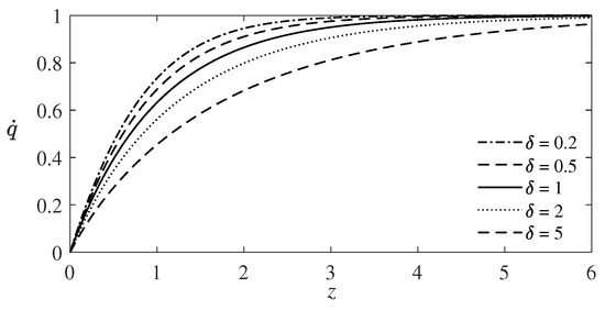
Figure 1. Graphs of the function $\dot{q}$ in the solution of problem (41) for different values of the parameter $\delta$.

Taking the limit in Equation (41) as $\delta \to 0$, one arrives at the problem of a critical point for the Prandtl boundary layer equations studied by K. Hiemenz [24]. In References [29,30], the existence of a solution of the problem (41) for $0<\delta \le 1$ was proven, and the asymptotic behavior of its solution for $\delta \to 0$ was constructed in the form of an asymptotic series $q=q_0+\delta q_1+{\delta }^2{q}_2+\cdots$, where $q_0$ is the Hiemenz solution. (Notice that for $\delta =1$ this problem has an exact solution $q=z+exp(-z)-1$).

The fact of the existence of a regular limit of the solution of problem (41) for $\delta \to 0$ is non-trivial, since the parameter $\delta$ is a multiplier in the highest derivative. Small values of $\delta$ correspond to small values of the normalized coefficient of the relaxation viscosity $\kappa$.

6.4. Group Foliation with Respect to $X_h$

Noticing that the generator $X_h$ coincides with the generator admitted by the boundary layer equations [26], one finds that the automorphic system of equations corresponding to the generator $X_h$ is

$$u_x+v_y=\omega (x,u),u_y=\phi (x,u),u{u}_x+v{u}_y=\psi (x,u).$$

(42)

Compatibility of the overdetermined system of equations consisting of systems (38) and (42) lead to the conditions that

$$\omega =0,\psi =\frac{\chi \phi {\phi }_u+u{\left(\phi {\phi }_u\right)}_x-P}{1-{\left(\phi {\phi }_u\right)}_u},$$

and the resolving equation

$${\phi }^2{\left(\frac{\psi }{\phi }\right)}_u-u{\phi }_x=0.$$

(43)

Calculations show that the resolving equation admits a Lie group only when $P=\alpha x+\beta$. The admitted generator has the form

$$X=k_1(u{\partial }_u+x{\partial }_x+\phi {\partial }_{\phi })+k_2{\partial }_x,$$

where the constants $k_1$ and $k_2$ satisfy the condition

$$\alpha k_2-\beta k_1=0.$$

6.5. Equation (38) in Mises Coordinates

Consider the system of boundary layer Equation (21) in the stationary case

$$u{u}_x+v{u}_y=-P+u_{yy},u_x+v_y=0,$$

(44)

where P is a given function of x. The second equation in (44) allows one to introduce the stream function $\psi (x,y)$ using the relations ${\psi }_y=u,$ and ${\psi }_x=-v$. Making the change in this system to the new independent variable $\psi$ instead of y, and denoting $u(x,y)=U(x,\psi (x,y\left)\right)$, one obtains that the function $U(x,\psi )$ satisfies the equation

$${\left(U^2\right)}_x=U{\left(U^2\right)}_{\psi \psi }-2P.$$

(45)

The variables x and $\psi$ are called Mises’s variables. They are widely used in the theory of the boundary layer [24]. The system of quasilinear Equation (44) does not have a certain type, which complicates its study. In contrast, Equation (45) is a parabolic equation in which x plays the role of an evolutionary variable.

Consider system (38). Using the change

$$u(x,y)=U(x,\psi (x,y)),u(x,y)-u_{yy}(x,y)=W(x,\psi (x,y)),$$

one comes to the equations in the Mises variables

$$U\left(\frac{\partial W}{\partial x}-\frac{\chi }{2}\frac{{\partial }^2\left(U^2\right)}{\partial {\psi }^2}\right)+P=0,\frac{U}{2}\frac{{\partial }^2\left(U^2\right)}{\partial {\psi }^2}=U-W.$$

(46)

The kernel of admitted Lie algebras of Equation (46) consists of the generator

$${\partial }_{\psi }.$$

Extensions of the kernel are defined by the generator

$$X=k_1(x{\partial }_x+\psi {\partial }_{\psi }+U{\partial }_U+W{\partial }_W)+k_2{\partial }_x,$$

where the constants $k_1$ and $k_2$ satisfy the classifying equation

$$(x{P}^{\prime }-P)k_1+P^{\prime }{k}_2=0.$$

If $P^{\prime }\ne 0$, then an extension only occurs for $P=qx$, where $q\ne 0$ is constant, and the extension of the kernel of admitted Lie algebras is defined by the generator

$$x{\partial }_x+\psi {\partial }_{\psi }+U{\partial }_U+W{\partial }_W.$$

Here, the equivalence transformation corresponding to the shift of x has been used. If $P^{\prime }=0$ and $P\ne 0$, then the extension of the kernel of admitted Lie algebras is defined by the generator

$${\partial }_x,$$

and for $P=0$ there is one more admitted generator

$$x{\partial }_x+\psi {\partial }_{\psi }+U{\partial }_U+W{\partial }_W.$$

Remark 2.

It should be noted here that the transition to the Mises coordinates led us to the reduction of the infinite part of the Lie algebra admitted by Equation (38). This property is one of the main reason of the application of the foliation.

For constructing invariant solutions of system (46) one needs to study the Lie algebra

$$X_1={\partial }_{\psi },X_2={\partial }_x,X_3=x{\partial }_x+\psi {\partial }_{\psi }+U{\partial }_U+W{\partial }_W.$$

An optimal system of one-dimensional subalgebras of this Lie algebra consists of the subalgebras

$$\left\{X_1\right\},\{X_2+\alpha X_1\},\left\{X_3\right\}.$$

An invariant solution with respect to $X_1$ is trivial, and provides that

$$u=u\left(x\right).$$

A solution invariant with respect to $X_2+\alpha X_1$ has the representation

$$U=U\left(z\right),W=W\left(z\right),z=\psi -\alpha x.$$

Substituting this representation into (46), one finds that

$$W=U(1-{\left(U^2\right)}^{″},$$

and the function $S=U^2$ satisfies the second-order ordinary differential equation

$$\alpha (4S{S}^{″}-S^{\prime 2}-4S)+8zP=4\chi S^{\prime }+4q,$$

where q is constant of integration. In particular, if $\alpha =0$, one finds

$$\int \frac{d\psi }{\sqrt{P{\psi }^2-q\psi +q_0}}={\chi }^{-1/2}y.$$

A solution invariant with respect to $X_3$ has the representation

$$U=x{U}_0\left(z\right),W=x{W}_0\left(z\right),z=\psi /x.$$

The reduced system becomes

$$W_0=U_0(1-{\left(U_0^2\right)}^{″}),$$

$$z{U}_0^2{U}_0^{‴}+U_0(4z{U}_0^{\prime }-U_0-\chi )U_0^{″}+z{U}^{\prime 3}-(U_0+\chi )U_0^{\prime 2}-z{U}_0^{\prime }+U_0=0.$$

(47)

One particular solution of the latter equation is

$$U_0=\beta \left(z+\frac{\chi \beta }{1-{\beta }^2}\right),$$

(48)

where $\beta \ne \pm 1$ is constant.

The solution (48) was used for testing a Runge-Kutta code for finding a solution of Equation (47). The results of the calculations are presented in Figure 2. In these calculations, solutions of Equation (47) were found using the same first two initial values of the function $U_0\left(z\right)$ at the point $z=a$:

$$U_0\left(a\right)=\beta \left(a+\frac{\chi \beta }{1-{\beta }^2}\right),U_0^{\prime }\left(a\right)=\beta .$$

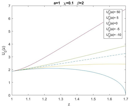
Figure 2. Solution $U_0\left(z\right)$ of Equation (47) for different values of $U_0^{″}\left(a\right):-10;-5;0;5;50$, presented in bottom-up order.

The graphs are presented for the following data: $a=1$, $\beta =2$, $\chi =0.1$ and the values of $U_0^{″}\left(a\right)$:

$$U_0^{″}\left(a\right):-10;-5;0;5;50.$$

In Figure 2 these graphs are presented in bottom-up order. Notice that $U_0^{″}\left(a\right)=0$ corresponds to the exact solution (48). From the calculations presented in Figure 2 one can note that the increase of the second-order derivative in the initial data leads to the solution, which for large values of z becomes close to linear.

7. Group Classification of the Boundary Layer Equations of Rivlin-Ericksen Fluids

Similar as for Equation (7), one derives that the classifying equation for the admitted Lie group is

$$k_1(x{P}_x-P)+k_3{P}_t+\xi P_x=-{\xi }^{″},$$

where

$$\xi =\xi \left(t\right),h=h\left(t\right),$$

and the generator has the form

$$X=k_1(u{\partial }_u+x{\partial }_x)+k_3{\partial }_t+\left(h{\partial }_y+h^{\prime }{\partial }_v\right)+({\xi }^{\prime }{\partial }_u+\xi {\partial }_x).$$

Hence, the kernel of admitted Lie algebras is defined by the generators

$$X_h=h{\partial }_y+h^{\prime }{\partial }_v.$$

Extensions of the kernel of admitted Lie algebras are the same as for Equation (7).

8. Discussion

8.1. Voitkunskii-Amfilokhiev-Pavlovskii Model

In Reference [23], a hereditary model of the motion of aqueous polymer solutions was formulated. It contains an integral operator of Volterra type and contains an additional material constant relaxation time of tangential stresses. In Reference [13], the equations of this model are reduced to the system of differential equations

$$\theta \frac{\partial }{\partial t}\frac{d\mathbf{v}}{dt}+\frac{d\mathbf{v}}{dt}=-\frac{\theta }{\rho }\frac{\partial \nabla p}{\partial t}-\frac{1}{\rho }\nabla p+\nu \theta \frac{\partial \Delta \mathbf{v}}{\partial t}+\nu \Delta \mathbf{v}+\kappa \frac{d\Delta \mathbf{v}}{dt},div\mathbf{v}=0,$$

(49)

where $\theta >0$ is a constant relaxation time. After reduction of system (49) to dimensionless variables, another (in addition to $\chi$) dimensionless parameter $\vartheta =\theta \nu /\kappa$ arises, which does not depend on the flow characteristics and is determined only by the properties of the medium. It can be small, and then a new problem of constructing an unsteady boundary layer for system (49) localized near the plane $t=0$ arises.

8.2. Blasius Problem

The classic problem of boundary layer theory is the Blasius problem on the uniform flow around a rectilinear plate under zero angle of attack [24]. This problem has a self-similar solution. Below an analogue of this problem is formulated for system (38), with $P=0$ written in Mises variables.

The problem is to find a solution of the system

$$\frac{\partial W}{\partial x}-\frac{\chi }{2}\frac{{\partial }^2\left(U^2\right)}{\partial {\psi }^2}=0,\frac{U}{2}\frac{{\partial }^2\left(U^2\right)}{\partial {\psi }^2}=U-W$$

(50)

in the half strip $S_l=\{x,\psi :0<x<l,\psi >\}$, satisfying the initial and boundary conditions

$$W=W_0\left(\psi \right),x=0,\psi \ge 0,$$

(51)

$$U=0,\psi =0;U\to 1,\psi \to \infty ,0\le x\le l.$$

(52)

In contrast to the Blasius problem, the problem (50)–(52) does not have self-similar solutions. Nevertheless, it is quite observable. For a given function W, the second equation of system (50) can be considered as an ordinary differential equation for the function U with respect to the variable $\psi$. A solution of the boundary value problem (52) for this equation forms the operator $U=F\left[W\right]$. Integrating the first Equation (50) with respect to x with the initial condition (51), one arrives at the operator equation

$$W(x,\psi )=W_0\left(\psi \right)+\frac{\chi }{2}\frac{{\partial }^2\left\{F{\left[W(x,\psi )\right]}^2\right\}}{\partial {\psi }^2}.$$

(53)

There is reason to believe that under the smoothness conditions and consistency on the function $W_0\left(\psi \right)$, the problem (50)–(52) possesses a solution for any $l>0$. It should be noted that the self-similar Blasius solution [24] has an unremovable defect: the transverse velocity tends to infinity when approaching the edge of the plate. We hope that by satisfying the condition ${\psi }^{-1/2}{W}_0\left(\psi \right)\in C^2[0,\infty )$, the Equation (53) has a solution which corresponds to a regular solution of the analog of the Blasius problem for the boundary layer system of Equation (38).

8.3. Separation

One of the central problems in the classical theory of the boundary layer is the problem of separation of the boundary layer. It is known that if the inequality $p_x\ge a>0$ for $x>0$ is satisfied, then there is an $x_{*}$ such that the solution of system (4) cannot be prolonged for the values of $x>x_{*}$ [24,31]. We believe that the condition of the positiveness of the function $p_x$ is also sufficient for the separation of the boundary layer in the Pavlovskii model of the motion of aqueous polymer solutions and in the Rivlin-Ericksen model of a second-order fluid. An interesting question is the dependence of the value $x_{*}$ on the parameter $\chi$.

9. Conclusions

The main results of our study are the construction of boundary layer equations of two mathematical models of the flow of aqueous polymer solutions [11,12], and the application of the group analysis method to their study.

In the previous section we have formulated three unsolved problems, which outline the plan of future analysis. In addition, we will be studying invariant and partially invariant solutions of system (6) of the boundary layer Rivlin-Ericksen model.

Our analysis allowed us to give a complete classification of invariant solutions of the boundary layer equations of two models describing the behaviour of polymer solutions. The solutions presented make it possible to evaluate the effect of polymer additives on the qualitative flow pattern in the boundary layer. In addition, they can be used as tests for developing numerical methods for solving systems of degenerate equations, which are systems (4) and (6).

References

- Toms, B.A. Some observations on the flow of linear polymer solutions through straight tubes at large Reynolds numbers. In Proceedings of the First International Congress on Rheology, Scheveningen, The Netherlands, 21–24 September 1948; Sissakian, A.N., Pogosyan, G.S.S., Eds.; North-Holland Publishing Company: Amsterdam, The Netherlands, 1948; Volume 2, pp. 135–141. [Google Scholar]
- Gupta, M.K.; Metzner, A.B.; Hartnett, J.P. Turbulent heat-transfer characteristics of viscoelastic fluids. Int. J. Heat Mass Transf. 1967, 10, 1211–1224. [Google Scholar] [CrossRef]
- Barenblatt, G.I.; Kalashnikov, V.N. Effect of high-molecular formations on turbulence in dilute polymer solutions. Fluid Dyn. 1968, 3, 45–48. [Google Scholar] [CrossRef]
- Barnes, H.A.; Townsend, P.; Walters, K. Flow of non-Newtonian liquids under a varying pressure gradient. Nature 1969, 224, 585–587. [Google Scholar] [CrossRef]
- Pisolkar, V.G. Effect of drag reducing additives on pressure loss across transitions. Nature 1970, 225, 936–937. [Google Scholar] [CrossRef] [PubMed]
- Amfilokhiev, V.B.; Pavlovskii, V.A. Experimental data on laminar-turbulent transition for flows of polymer solutions in pipes. Tr. Leningr. Korablestr. Inst. 1976, 104, 3–5. (In Russian) [Google Scholar]
- Amfilokhiev, V.B.; Pavlovskii, V.A.; Mazaeva, N.P.; Khodorkovskii, Y.S. Flows of polymer solutions in the presence of convective accelerations. Tr. Leningr. Korablestr. Inst. 1975, 96, 3–9. (In Russian) [Google Scholar]
- Sadicoff, B.L.; Brandao, E.M.; Lucas, E.F. Rheological behaviour of poly (Acrylamide-G-propylene oxide) solutions: Effect of hydrophobic content, temperature and salt addition. Int. J. Polym. Mater. 2000, 47, 399–406. [Google Scholar] [CrossRef]
- Fu, Z.; Otsuki, T.; Motozawa, M.; Kurosawa, T.; Yu, B.; Kawaguchi, Y. Experimental investigation of polymer diffusion in the drag-reduced turbulent channel flow of inhomogeneous solution. Int. J. Heat. Mass. Transfer. 2014, 77, 860–873. [Google Scholar] [CrossRef]
- Han, W.J.; Dong, Y.Z.; Choi, H.J. Applications of water-soluble polymers in turbulent drag reduction. Processes 2017, 5, 24. [Google Scholar] [CrossRef]
- Pavlovskii, V.A. Theoretical description of weak aqueous polymer solutions. Dokl. Akad. Nauk SSSR 1971, 200, 809–812. [Google Scholar]
- Rivlin, R.S.; Ericksen, J.L. Stress-deformation relations for isotropic materials. J. Ration. Mech. Anal. 1955, 4, 323–425. [Google Scholar] [CrossRef]
- Frolovskaya, O.A.; Pukhnachev, V.V. Analysis of the Models of Motion of Aqueous Solutions of Polymers on the Basis of Their Exact Solutions. Polymers 2018, 10, 684. [Google Scholar] [CrossRef] [PubMed]
- Oskolkov, A.P. On the uniqueness and global solvability of boundary-value problems for the equations of motion of aqueous solutions of polymers. Zap. Nauchn. Semin. LOMI 1973, 38, 98–136. (In Russian) [Google Scholar] [CrossRef]
- Oskolkov, A.P. Theory of nonstationary flows of Kelvin-Voigt fluids. J. Sov. Math. 1985, 28, 751–758. [Google Scholar] [CrossRef]
- Galdi, G.P.; Dalsen, M.G.V.; Sauer, N. Existence and uniqueness of classical solutions of equations of motion for second-grade fluids. Arch. Ration. Mech. Anal. 1993, 124, 221–237. [Google Scholar] [CrossRef]
- Roux, C.L. Existence and Uniqueness of the Flow of Second-Grade Fluids with Slip Boundary Conditions. Arch. Ration. Mech. Anal. 1999, 148, 309–356. [Google Scholar] [CrossRef]
- Zvyagin, A.V. Solvability for equations of motion of weak aqueous polymer solutions with objective derivative. Nonlinear Anal. Theory Methods Appl. 2013, 90, 70–85. [Google Scholar] [CrossRef]
- Zvyagin, A.V. Analysis of the solvability of a stationary model of motion of weak aqueous polymer solutions. Vestn. Voronezh. Gos. Univ. Ser. Fiz. Mat. 2011, 1, 147–156. (In Russian) [Google Scholar]
- Bozhkov, Y.D.; Pukhnachev, V.V. Group analysis of equations of motion of aqueous solutions of polymers. Dokl. Phys. 2015, 60, 77–80. [Google Scholar] [CrossRef]
- Bozhkov, Y.D.; Pukhnachev, V.V.; Pukhnacheva, T.P. Mathematical models of polymer solutions motion and their symmetries. AIP Conf. Proc. 2015, 1684, 77–80. [Google Scholar] [CrossRef]
- Pukhnachev, V.V.; Frolovskaya, O.A. On the Voitkunskii-Amfilokhiev-Pavlovskii model of motion of aqueous polymer solutions. Proc. Steklov Inst. Math. 2018, 300, 168–181. [Google Scholar] [CrossRef]
- Voitkunskii, Y.I.; Amfilokhiev, V.B.; Pavlovskii, V.A. Equations of motion of a fluid, with its relaxation properties taken into account. Tr. Leningr. Korablestr. Inst. 1970, 69, 19–26. (In Russian) [Google Scholar]
- Schlichting, H. Boundary-Layer Theory, 7th ed.; McGraw-Hill, Inc.: New York, NY, USA, 1979. [Google Scholar]
- Sadeghy, K.; Khabazi, N.; Taghavi, S.M. The Boundary Layer Flows of a Rivlin-Ericksen Fluid. In New Trends in Fluid Mechanics Research; Zhuang, F.G., Li, J.C., Eds.; Springer: Berlin, Germany, 2007. [Google Scholar]
- Ovsiannikov, L.V. Group Analysis of Differential Equations; English Translation; Ames, W.F., Ed.; Nauka: Moscow, Russia, 1978. [Google Scholar]
- Patera, J.; Winternitz, P. Subalgebras of real three- and four-dimensional Lie algebras. J. Math. Phys. 1977, 18, 1449–1455. [Google Scholar] [CrossRef]
- Pukhnachev, V.V.; Frolovskaya, O.A.; Petrova, A.G. Polymer solutions and their mathematical models. Proc. High Sch. North Cauc. Reg. Nat. Sci. 2020, 84–93. (In Russian) [Google Scholar]
- Petrova, A.G. On the Unique Solvability of the problem of the flow of an aqueous solution of polymers near a critical point. Math. Notes 2019, 106, 784–793. [Google Scholar] [CrossRef]
- Petrova, A.G. Justification of asymptotic decomposition of a solution for the problem of the motion of weak solutions of polymers near a critical point. Sib. Electron. Math. Rep. 2020, 17, 313–317. (In Russian) [Google Scholar] [CrossRef]
- Oleinik, O.A. On a system of equations in boundary layer theory. USSR Comput. Math. Math. Phys. 1963, 3, 650–673. [Google Scholar] [CrossRef]
© 2020 by the authors. Licensee MDPI, Basel, Switzerland. This article is an open access article distributed under the terms and conditions of the Creative Commons Attribution (CC BY) license (http://creativecommons.org/licenses/by/4.0/).