Abstract
We analyze constraints on the anomalous couplings from B-physics experiments, performing a correlated analysis and allowing all anomalous couplings to differ simultaneously from their Standard Model (SM) values. The B-physics observables allow one to probe three linear combinations out of the four anomalous couplings, which parameterize the vertex under the assumption that the SM symmetries remain the symmetries of the effective theory. The constraints in this work are obtained by taking into account the following B-physics observables: the oscillations, the leptonic decays, the inclusive radiative decays, and the differential branching fractions in the semileptonic inclusive and exclusive decays at small , with q the momentum of the pair. We find that the SM values of the anomalous couplings belong to the 95% CL allowed region obtained this way, but lie beyond the 68% allowed region. We also report that the distributions of the anomalous couplings obtained within our scenario differ from the results of the 1D scenario, when only one of the couplings is allowed to deviate from its SM value.
1. Introduction
The top quark is the heaviest of all known elementary particles and may be expected to have large couplings with physics beyond the Standard Model (BSM). One of the possibilities to probe BSM physics is to study the anomalous structure of the vertex.
At the scale , the effects of BSM interactions may be parameterized in the framework of an effective field theory by a tower of higher dimension operators constructed from the SM fields and obeying the SM symmetries [1]. The most general Lagrangian of the vertex has the following form [2]:
where , , g is the gauge coupling. The Lagrangian (1) corresponds to the choice of the covariant derivative acting on a left quark doublet with weak hypercharge Y in the form:
The anomalous couplings , , , and are induced by dimension-six operators of the effective theory. In the SM, all anomalous couplings have zero values: . (For convenience, we provide a comparison with the anomalous couplings used in other papers: One finds [3][4] [2]. For other couplings, [3][4] [2], [3][4] [2], and [3][4] [2].) Notice that vanishing of the anomalous couplings in the SM Lagrangian does not forbid the appearance of the corresponding Lorentz structures in the amplitude through radiative corrections [5].
The gauge invariance leads to the appearance of the anomalous structures not only in the , but also in other vertices [4]. Imposing a number of constraints (e.g., no tree-level FCNC), these structures are given in terms of the same anomalous couplings as in Equation (1) and the appropriate CKMmatrix elements.
The anomalous couplings are in general complex numbers [3,5,6,7]; this paper studies the constraints on the couplings in a restricted scenario assuming that they are real quantities.
Obtaining experimental bounds on the anomalous couplings is an important direction in the search for new physics. Such bounds may be obtained from different sources: e.g., from the direct production of top quarks at hadron colliders, where weak processes are the main mechanism of the single t-production [8]. Another promising way is the indirect probing of the anomalous couplings from FCNC processes in B-physics: here, the virtual top often gives the leading contribution, thus opening the possibility to constrain its anomalous couplings [3,4,9]. This paper follows the line of the analysis of [3] and studies more closely the correlations between the anomalous couplings that can be obtained from the B-physics data.
2. Effective Lagrangian for Weak FCNC -Decays
For the description of weak B-decays, an appropriate physics scale is GeV; all particles with much heavier masses are not dynamical and may be integrated out within the formalism based on the operator product expansion. The light degrees of freedom, such as the quarks, the photon, and the gluons are dynamical degrees of freedom. For FCNC B-decays, this approach leads to the effective Lagrangian, which involves operators built up of the light degrees of freedom (for details and the full set of the basis operators, see [10,11,12] and the discussion in [13,14,15]):
The operators in (3) are four-quark operators containing quark fields , b, , c with different color contractions. One also has the analogous four-quark operators with the c-quark replaced by the u-quark; the corresponding Wilson coefficients are however strongly CKM suppressed as . For instance, the operators generating the charming loops are:
The operators are bilinear in quark fields:
The -dependent Wilson coefficients at the scale encode the effects of heavy particles; in the SM, these are , Z, and the t-quark, but in the extensions of the SM, other heavy particles contribute, thus changing the values of the Wilson coefficients. One can write:
where the additional terms reflect the new physics contributions. The SM Wilson coefficients have the values: , , , . We do not consider in our analysis the operators with the opposite chirality compared to , respectively: In the SM, , , and the corrections induced by the anomalous couplings are proportional to and are thus much smaller than .
The additions to the Wilson coefficients due to the anomalous couplings were obtained in [3,4]; they are linear functions of the following anomalous couplings:
For the explicit formulas, we refer to Appendix B of [3], and we apply those formulas for the matching scale . We also use the B- oscillations; the correction to the corresponding amplitude due to the anomalous couplings was calculated in [9]. It is noteworthy that it contains only two anomalous couplings, and .
B-meson observables, in addition to the Wilson coefficients, involve the amplitudes of the effective operators; the latter contain complicated hadron effects. Therefore, in practice, only those processes involving B-mesons, where the hadron uncertainties are kept under reasonable theoretical control, may be used for probing the anomalous couplings. A plausible strategy for the purpose of searching for New Physics (NP) is to avoid, e.g., hadronic weak B-meson decays.
An unavoidable difficulty in the theoretical description of FCNC B-decays is the calculation of the contributions generated by the four-quark operators in (3), the so-called charming loops, especially their nonfactorizable parts [16,17,18,19]. Recall that the contribution of the virtual charm to FCNC B-decays is not CKM suppressed compared to the contribution of the top quark. In the amplitudes of -decays, the factorizable charm contribution is governed by the linear combination of the Wilson coefficients which is strongly scale dependent. For instance, at , is compared with the value that governs a part of the top quark contribution. Indeed, at small , with q the momentum of the pair, there is a sizeable numerical suppression of the charming loops compared to the top contribution, but this suppression is the subject of the precise choice of the scale , indicating the importance of higher order QCDcorrections. As increases, the charm contribution rises much faster than that of the top; the charm takes over the top when one approaches the charmonia region [16]. Finally, for the purpose of the search for NP, one can use FCNC B-decays below the charm threshold as soon as one has reliable theoretical predictions for the form factors and for the contribution of the charming loops.
For our further analysis, it is important to pay attention to the following facts:
- (i)
- the coefficients and , as well as the amplitude of the B- oscillations do not get contributions from and .
- (ii)
- the coefficient involves only one linear combination of and .
Therefore, in practice, precision measurements of () from B-physics allows one to get access to , , and one specific linear combination of and , determined by .
3. Bounds on Anomalous Couplings
When studying constraints on the anomalous couplings, both from direct top quark production and from B-physics, one often considers different scenarios, depending on how many couplings are allowed to vary from their zero SM values. For instance, one-dimensional scenarios, when only one of the couplings is allowed to be nonzero, are well known [3,4,8]. Using such an approach, however, one does not access those regions where different anomalous couplings may have strongly correlated values far away from their zero SM values. We therefore follow here a different strategy: we allow all couplings to be nonzero and obtain the corresponding bounds from the data.
As already noticed above, only those B-decay channels, where theoretical QCD uncertainties are kept under control, may be used for the extraction of the anomalous couplings. We use for our analysis the following channels:
- oscillations (see, e.g., [20]): We consider the ratio of in the theory with anomalous couplings over in the SM; its dependence on the anomalous couplings was calculated in [9]. We fit this quantity to the ratio of the experimental [21] over its lattice determination [22].
- : data from [21] and theoretical estimates from [23].
- , with q the momentum of the pair: data from [21] and theoretical inputs from [3].
- : data from [21,24] and the theoretical predictions from [23] (see also [25]).
- : data from [26] in the lowest -bins: GeV and GeV. The differential distributions and asymmetries for these decays were calculated in [27]; convenient formulas parameterizing the theoretical results as functions of the Wilson coefficients were given in [28]. In this channel, the accuracy of the experimental results is slightly better than that of the theoretical predictions: the form factors at small necessary for calculating the differential branching fractions of interest come mainly from Light-Cone QCD Sum Rules (LCSR); this method unfortunately does not allow a solid control over the systematic uncertainties of the calculated form factors [29,30] (cf. [31,32]). We assign a 15% uncertainty on the LCSR predictions for the form factors, yielding a 30% uncertainty on the differential distributions.
- : We make use of the LHCb data [33] in two bins, GeV and GeV (see also [34]). The necessary form factors come from LCSRs, e.g., [16,31,32]. The most recent analysis [32] yields the form factors and . These numbers are somewhat smaller than those from the previous analysis [16]: and . It is also noteworthy that the uncertainties reported in [32] are considerably larger compared to the previous estimates. Taking into account the already mentioned problem with the assignment of uncertainties within QCD sum rules, for the analysis, we employ the form factor parametrizations from [35], which correspond to and , and assign to them a 15% theoretical uncertainty. The full contribution of the charming loops, including the factorizable and the nonfactorizable effects, from [16], is taken into account. Convenient expressions for (in GeV) as functions of the additions to the Wilson coefficients in two bins of low- are given below:
The amplitudes of these processes involve, via , , and , the anomalous couplings , , but only one linear combination of the couplings and :
with and at the scale of 5 GeV [3]. In what follows, we obtain experimental bounds on f, , and at the scale of from the B-physics data listed above.
With the theoretical expressions for the observables of interest as functions of the anomalous couplings at hand, we proceed as follows: for a combination of the independent observables with the calculated theoretical dependence on the set of the anomalous couplings F in the form , the experimental averages , and the uncertainties , we obtain the combined probability distribution of F as follows:
where is obtained by combining the experimental and the theoretical uncertainties of the corresponding observable as .
Integrating these distributions over one of the couplings, we obtain normalized 2D distributions of two other couplings shown in Figure 1. In all cases, the SM values belong to the 95% CL; however, they are outside the 68% CL area.
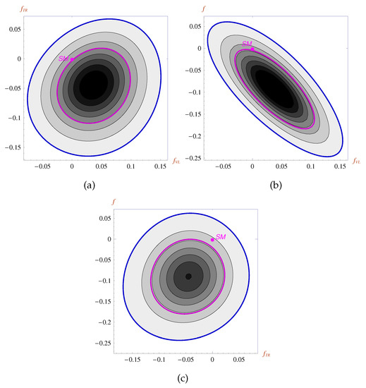
Figure 1.
The topographic maps of the 2D distributions of the anomalous couplings at the scale are obtained by integrating the 3D distribution over the third coupling: (a) -; (b) -f; and (c) -f. In each plot, the blue external contour embraces the 95% CL region; the violet contour embraces the 68% CL region. The black contours correspond to the values .
Finally, Figure 2 gives a one-dimensional distribution of the individual coupling, obtained by integrating the 3D distribution over other couplings. We emphasize that these 1D distributions differ from the 1D distributions obtained by setting all other couplings to their SM values.
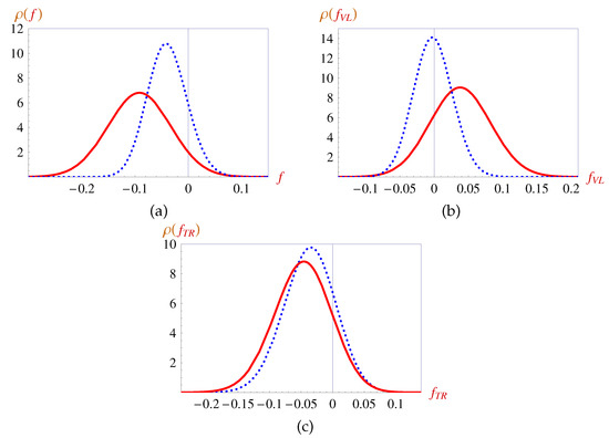
Figure 2.
The 1D distributions obtained by integrating the 3D distributions (red solid lines): (a) f; (b) ; and (c) . For comparison, the blue dashed lines show the distributions obtained by setting all other anomalous couplings to zero. The results present the distributions of the anomalous couplings at the matching scale .
4. Discussion and Conclusions
We presented a detailed analysis of the anomalous couplings based on a broad range of B-physics data allowing all of them to differ simultaneously from zero. Our conclusions may be summarized as follows:
- Taking into account that any analysis of the B-physics data involves the theoretical calculation of complicated nonperturbative QCD effects (e.g., related to B-meson in the initial state, light mesons in the final state, charming-loops, and charmonia resonances), only those modes where such effects may be controlled with good accuracy are appropriate for the analysis of the anomalous couplings. Presently, such effects are limited to FCNC radiative or semileptonic B-decays in the region of small momentum transfers of the pair, purely leptonic B-decays, and the oscillation of neutral B-mesons. In other interesting processes/kinematic regions, where the gluon penguin operator or four-quark operators provide sizeable or dominant contributions, the nonperturbative QCD effects are very difficult to calculate with good accuracy; therefore, such processes are not suitable for the analysis of the anomalous couplings from the data. Consequently, B-decays can provide bounds on three quantities: the anomalous couplings , , and one linear combination f of two other couplings, and , which appears in the Wilson coefficient .
- Allowing simultaneous deviations of all anomalous couplings from zero and calculating the 1D distributions by integrating the 3D distributions lead to rather visible differences from the 1D distributions obtained by allowing only one anomalous coupling to take a non-SM value and keeping all other couplings at zero; see Figure 2.
- Figure 1 and Figure 2 show our results for the distributions of the anomalous couplings at the scale of . In all considered 2D and 1D distributions, the SM values of the couplings belong to the region allowed at the 95% CL. However, the SM values lie beyond the 68% CL region of the anomalous couplings. To obtain further constraints on the anomalous couplings, in particular, for constraining the couplings and , separately, combining bounds on the anomalous couplings from the B-physics data with the direct bounds from single top quark production is a promising route to new physics [36,37,38]. The direct constraints on the anomalous couplings from LHC data depend on the scenarios of the anomalous couplings (1D or 2D) used in the analysis. Within 1D scenarios, indirect constraints from B-physics experiments are presently much more restrictive compared to the direct top quark measurements [37].
Author Contributions
Conceptualization and methodology of the paper, A.K. and D.M.; numerical calculations, A.K.; analysis, A.K. and D.M.; writing–original draft preparation, A.K. and D.M.; writing–review and editing, D.M. All authors have read and agreed to the published version of the manuscript.
Funding
This research was funded by Russian Foundation of Basic Research (RFBR) Grant 19-52-15022 (A.K. and D.M.) and by Russian Science Foundation (RSCF) Grant 16-12-10280 (A.K., Section 3).
Acknowledgments
We are grateful to C. Bobeth, E. Boos, V. Bunichev, M. Dubinin, L. Dudko, P. Mandrik, D. Savin, and D. van Dyk for stimulating and interesting discussions. We thank the Organizers of the MIAPP program “Deciphering Strong-Interaction Phenomenology through Precision Hadron-Spectroscopy” held 7-31 October 2019 at the Excellence Cluster “Universe” in Garching, Germany, for financial support of our participation at this workshop, where a major part of this work was done.
Conflicts of Interest
The authors declare no conflict of interest.
References
- Buchmuller, W.; Wyler, D. Effective Lagrangian Analysis of New Interactions and Flavor Conservation. Nucl. Phys. B 1986, 268, 621. [Google Scholar] [CrossRef]
- Kane, G.L.; Ladinsky, G.A.; Yuan, C.P. Using the top quark for testing Standard Model polarization and CP predictions. Phys. Rev. D 1992, 45, 124. [Google Scholar] [CrossRef] [PubMed]
- Drobnak, J.; Fajfer, S.; Kamenik, J.F. Probing anomalous tWb interactions with rare B decays. Nucl. Phys. B 2012, 855, 82. [Google Scholar] [CrossRef]
- Grzadkowski, B.; Misiak, M. Anomalous Wtb coupling effects in the weak radiative B-meson decay. Phys. Rev. D 2008, 78, 077501, Erratum in Phys. Rev. D 2011, 84, 059903. [Google Scholar] [CrossRef]
- Fischer, M.; Groote, S.; Körner, J.G. T-odd correlations in polarized top quark decays in the sequential decay t(↑)→XbW(→l++νl) and in the quasi three-body decay t(↑)→Xb+l++νl). Phys. Rev. D 2018, 97, 093001. [Google Scholar] [CrossRef]
- Groote, S.; Körner, J.G. Positivity bound on the imaginary part of the right-chiral tensor coupling gR in polarized top quark decay. Phys. Rev. D 2017, 96, 111301. [Google Scholar] [CrossRef]
- Alioli, S.; Cirigliano, V.; Dekens, W.; de Vries, J.; Mereghetti, E. Right-handed charged currents in the era of the Large Hadron Collider. JHEP 2017, 1705, 086. [Google Scholar] [CrossRef]
- Khachatryan, V.; Sirunyan, A.M.; Tumasyan, A.; Adam, W.; Aşılar, E.; Bergauer, T.; Brandstetter, J.; Brondolin, E.; Dragicevic, M.; Erö, J.; et al. Search for anomalous Wtb couplings and flavour-changing neutral currents in t-channel single top quark production in pp-collisions at = 7 and 8 TeV. JHEP 2017, 1702, 028. [Google Scholar] [CrossRef]
- Drobnak, J.; Fajfer, S.; Kamenik, J.F. Interplay of t→bW Decay and Bq Meson Mixing in Minimal Flavor Violating Models. Phys. Lett. B 2011, 701, 234. [Google Scholar] [CrossRef]
- Grinstein, B.; Savage, M.J.; Wise, M.B. B→X(s)e+e− in the Six Quark Model. Nucl. Phys. B 1989, 319, 271. [Google Scholar] [CrossRef]
- Buras, A.J.; Munz, M. Effective Hamiltonian for B→X(s)e+e− beyond leading logarithms in the NDR and HV schemes. Phys. Rev. D 1995, 52, 186. [Google Scholar] [CrossRef]
- Buchalla, G.; Buras, A.J.; Lautenbacher, M.E. Weak decays beyond leading logarithms. Rev. Mod. Phys. 1996, 68, 1125. [Google Scholar] [CrossRef]
- Altmannshofer, W.; Straub, D.M. New physics in b→s transitions after LHC run 1. Eur. Phys. J. C 2015, 75, 382. [Google Scholar] [CrossRef]
- Bobeth, C.; Misiak, M.; Urban, J. Matching conditions for b→sγ and b→s gluon in extensions of the standard model. Nucl. Phys. B 2000, 567, 153. [Google Scholar] [CrossRef]
- Bobeth, C.; Misiak, M.; Urban, J. Photonic penguins at two loops and mt dependence of BR[B→Xsl+l−]. Nucl. Phys. B 2000, 574, 291. [Google Scholar] [CrossRef]
- Khodjamirian, A.; Mannel, T.; Pivovarov, A.; Wang, Y.-M. Charm-loop effect in B→K(*)l+l− and B→K*γ. JHEP 2010, 9, 089. [Google Scholar] [CrossRef]
- Kozachuk, A.; Melikhov, D.; Nikitin, N. Rare FCNC radiative leptonic Bs,d→γl+l− decays in the standard model. Phys. Rev. D 2018, 97, 053007. [Google Scholar] [CrossRef]
- Kozachuk, A.; Melikhov, D. Revisiting nonfactorizable charm-loop effects in exclusive FCNC B-decays. Phys. Lett. B 2018, 786, 378. [Google Scholar] [CrossRef]
- Melikhov, D. Charming loops in exclusive rare FCNC B–decays. EPJ Web Conf. 2009, 222, 01007. [Google Scholar] [CrossRef][Green Version]
- Lenz, A.; Nierste, U.; Charles, J.; Descotes-Genon, S.; Jantsch, A.; Kaufhold, C.; Lacker, H.; Monteil, S.; Niess, V.; T’Jampens, S.; et al. Anatomy of New Physics in B-B¯ mixing. Phys. Rev. D 2011, 83, 036004. [Google Scholar] [CrossRef]
- Amhis, Y.; Banerjee, S.; Ben-Haim, E.; Bernlochner, F.; Bozek, A.; Bozzi, C.; Chrząszcz, M.; Dingfelder, J.; Duell, S.; Gersabeck, M.; et al. Averages of b-hadron, c-hadron, and π-lepton properties as of 2018. arXiv 2019, arXiv:1909.12524. [Google Scholar]
- Aoki, S.; Aoki, Y.; Becirevic, D.; Blum, T.; Colangelo, G.; Collins, S.; Morte, M.D.; Dimopoulos, P.; Durr, S.; Fukaya, H.; et al. FLAG Review 2019: Flavour Lattice Averaging Group (FLAG). Eur. Phys. J. C 2020, 80, 113. [Google Scholar] [CrossRef]
- Descotes-Genon, S.; Ghosh, D.; Matias, J.; Ramon, M. Exploring New Physics in the C7- plane. J. High Energy Phys. 2011, 1106, 099. [Google Scholar] [CrossRef]
- Aaij, R.; Adeva, B.; Adinolfi, M.; Ajaltouni, Z.; Akar, S.; Albrecht, J.; Alessio, F.; Alexander, M.; Ali, S.; Alkhazov, G.; et al. Measurement of the →μ+μ− branching fraction and effective lifetime and search for B0→μ+μ− decays. Phys. Rev. Lett. 2017, 118, 191801. [Google Scholar] [CrossRef]
- Hermann, T.; Misiak, M.; Steinhauser, M. Three-loop QCD corrections to Bs→μ+μ−. J. High Energy Phys. 2013, 1312, 097. [Google Scholar] [CrossRef]
- Aaij, R.; Adeva, B.; Adinolfi, M.; Ajaltouni, Z.; Akar, S.; Albrecht, J.; Alessio, F.; Alexander, M.; Ali, S.; Alkhazov, G.; et al. Measurements of the S-wave fraction in B0→K+π−μ+μ− decays and the B0→K*(892)0μ+μ− differential branching fraction. J. High Energy Phys. 2017, 1611, 047, Erratum in 2017, 1704, 142. [Google Scholar] [CrossRef]
- Altmannshofer, W.; Ball, P.; Bharucha, A.; Buras, A.; Straub, D.M.; Wick, M. Symmetries and asymmetries of B→K*μ+μ− decays in the Standard Model and beyond. J. High Energy Phys. 2009, 0901, 019. [Google Scholar] [CrossRef]
- Capdevila, B.; Crivellin, A.; Descotes-Genon, S.; Matias, J.; Virto, J. Patterns of New Physics in b→sl+l− transitions in the light of recent data. J. High Energy Phys. 2018, 1801, 093. [Google Scholar] [CrossRef]
- Melikhov, D. Hadron form factors from sum rules for vacuum-to-hadron correlators. Phys. Lett. B 2009, 671, 450. [Google Scholar] [CrossRef][Green Version]
- Lucha, W.; Melikhov, D.; Sazdjian, H.; Simula, S. Effective continuum threshold for vacuum-to-bound-state correlators. Phys. Rev. D 2009, 80, 114028. [Google Scholar] [CrossRef]
- Bharucha, A.; Straub, D.M.; Zwicky, R. B→Vl+l− in the Standard Model from light-cone sum rules. J. High Energy Phys. 2016, 1608, 098. [Google Scholar] [CrossRef]
- Gubernari, N.; Kokulu, A.; van Dyk, D. B→P and B→V Form Factors from B-Meson Light-Cone Sum Rules beyond Leading Twist. J. High Energy Phys. 2019, 1901, 150. [Google Scholar] [CrossRef]
- Aaij, R.; Amhis, Y.; Barsuk, S.; Callot, O.; He, J.; Kochebina, O.; Lefrançois, J.; Machefert, F.; Martin Sanchez, A.; Nicol, M.; et al. Differential branching fractions and isospin asymmetries of B→K(*)μ+μ− decays. J. High Energy Phys. 2014, 1406, 133. [Google Scholar] [CrossRef]
- Aaij, R.; Adeva, B.; Adinolfi, M.; Ajaltouni, Z.; Akar, S.; Albrecht, J.; Alessio, F.; Alexander, M.; Ali, S.; Alkhazov, G.; et al. Measurement of the phase difference between short- and long-distance amplitudes in the B+→K+μ+μ− decay. Eur. Phys. J. C 2017, 77, 161. [Google Scholar] [CrossRef] [PubMed]
- Bailey, J.A.; Bazavov, A.; Bernard, C.; Bouchard, C.M.; DeTar, C.; Du, D.; El-Khadra, A.X.; Foley, J.; Freeland, E.D.; Gámiz, E.; et al. B→Kl+l− Decay Form Factors from Three-Flavor Lattice QCD. Phys. Rev. D 2016, 93, 025026. [Google Scholar] [CrossRef]
- Dutta, S.; Goyal, A.; Kumar, M.; Mellado, B. Measuring anomalous Wtb couplings at e−p collider. Eur. Phys. J. 2015, C 75, 577. [Google Scholar] [CrossRef]
- Kozachuk, A. Combining direct and indirect constraints on anomalous Wtb couplings. EPJ Web Conf. 2019, 222, 04008. [Google Scholar] [CrossRef]
- Bißmann, S.; Erdmann, J.; Grunwald, C.; Hiller, G.; Kröninger, K. Constraining top quark couplings combining top quark and B decay observables. Eur. Phys. J. C 2020, 80, 136. [Google Scholar] [CrossRef]


© 2020 by the authors. Licensee MDPI, Basel, Switzerland. This article is an open access article distributed under the terms and conditions of the Creative Commons Attribution (CC BY) license (http://creativecommons.org/licenses/by/4.0/).