Investigation of the Thermal QCD Matter from Canonical Sectors

Abstract

We discuss the thermal phase structure of quantum chromodynamics (QCD) at zero real chemical potential (${\mu }_{\mathrm{R}}=0$) from the viewpoint of canonical sectors. The canonical sectors take the system to pieces of each elementary excitation mode and thus seem to be useful in the investigation of the confinement–deconfinement nature of QCD. Since the canonical sectors themselves are difficult to compute, we propose a convenient quantity which may determine the structural changes of the canonical sectors. We discuss the quantity qualitatively by adopting lattice QCD prediction for the phase structure with finite imaginary chemical potential. In addition, we numerically estimate this quantity by using the simple QCD effective model. It is shown that there should be a sharp change of the canonical sectors near the Roberge–Weiss endpoint temperature at ${\mu }_{\mathrm{R}}=0$. Then, the behavior of the quark number density at finite imaginary chemical potential plays a crucial role in clarifying the thermal QCD properties.

1. Introduction

Exploring the phase structure of quantum chromodynamics (QCD) at a finite temperature (T) and real chemical potential (${\mu }_{\mathrm{R}}$) is an important subject in elementary particle, hadron and nuclear physics and in astrophysics. Several studies have investigated the thermal QCD phase structure with ${\mu }_{\mathrm{R}}=0$ to date, but the full understanding of the system has not been obtained yet. Particularly, the understanding of the confinement–deconfinement nature of QCD is a long-standing problem; for example, see [1].

In the standard understanding of the confinement–deconfinement nature, the realistic thermal QCD matter at ${\mu }_{\mathrm{R}}=0$ is the crossover; there are no clear phase transitions. The Polyakov loop, which is a gauge-invariant holonomy, is usually employed to clarify the confinement–deconfinement nature since the Polyakov loop is directly related to the one-quark excitation free energy, at least in the pure gauge limit. Then, the confinement–deconfinement transition has a relation with the spontaneous breaking of ${\mathbb{Z}}_3$ symmetry. This is, of course, not clear in the realistic system with a finite quark mass because the relation between the Polyakov loop and the free energy is missed; for example, see [2] concerning this relation. There are also several investigations into the QCD confinement–deconfinement transition from topological viewpoints; see [1] for a review.

It is an interesting topic of study to investigate the confinement–deconfinement nature with a realistic quark mass based on topology; in this area, the idea of the topological order was used in [3]. In that study, the authors showed that the confinement and the deconfinement state at $T=0$ can be clarified by using the ground-state degeneracy which directly relates to the topological order. Of course, the ground-state degeneracy cannot be directly implemented to the thermal system, but it enhances our expectation that the QCD confinement–deconfinement nature is related to the topological phase transition even with a realistic quark mass. Since it is not necessary that the system has a singularity of local order parameters and thermodynamics quantities in the case of the topological phase transition, this expectation is not inconsistent with the crossover picture of realistic QCD. Actually, there have been some attempts to investigate the confinement–deconfinement nature based on this expectation [4,5,6].

In this paper, we employ the canonical ensemble to investigate the detailed structure of the thermal system since the partition function has almost all information of the thermal system, even if there are no singularities; see [7,8,9,10,11] for details of the canonical ensemble method in QCD. In other words, we attempt to find some interesting properties from the anatomy of the grand canonical partition function from the viewpoint of the canonical sectors. In [12], the authors showed that the investigation of canonical sectors represented by the Fourier decomposition is a useful and powerful tool to understand the QCD phase structure at a finite ${\mu }_{\mathrm{R}}$ with a sufficiently small T. This result enhances our expectation that the canonical ensemble can provide us with important information about the confinement–deconfinement nature of QCD even with a finite T. This paper is an extension of the paper [12] that explored the thermal QCD phase structure based on the canonical sectors. In addition, some previous studies have been based on the Fourier decomposition of the quark number density [13,14,15]. Those studies suggested that the chiral and/or deconfinement transitions affect Fourier coefficients determined from the quark number density. The difference between the previous studies and the present study is that we show clear connections between the canonical sectors and each component of the quark number density and investigate the influences of the phase structure at a finite $\theta$ to that at ${\mu }_{\mathrm{R}}=0$ from the viewpoint of the canonical sectors. The proposal of the convenient quantity that reflects the structure of the canonical sectors via the quark number density is also the main result of this work.

This paper is organized as follows. In the next section, we explain the construction of the canonical ensemble via the imaginary chemical potential region. Section 3 shows the known results of QCD with finite imaginary chemical potential. Our observations are shown in Section 4 and Section 5 is devoted to the discussion and summary.

2. Canonical Sectors

The important ingredient of the construction of the canonical ensemble is the imaginary chemical potential (${\mu }_{\mathrm{I}}$); see [16] for a review of studies into imaginary chemical potential. Below, we denote $\mu =({\mu }_{\mathrm{R}},{\mu }_{\mathrm{I}})$. Each canonical sector corresponding to the canonical partition function (${\mathcal{Z}}_{\mathrm{C}}$) with a fixed Q is given by

$$\begin{array}{cc}\hfill {\mathcal{Z}}_{\mathrm{C}}(T,Q)& =\frac{1}{2\pi }{\int }_{-\pi }^{\pi }d\theta e^{-iQ\theta }{\mathcal{Z}}_{\mathrm{GC}}(T,\theta )\hfill \\ \hfill & =\frac{1+z^Q+z^{2Q}}{2\pi }{\int }_{-\pi /3}^{\pi /3}d\theta e^{-iQ\theta }{\mathcal{Z}}_{\mathrm{GC}}(T,\theta )\hfill \\ & =\{\begin{array}{cc}\frac{3}{2\pi }{\int }_{-\pi /3}^{\pi /3}d\theta e^{-iQ\theta }{\mathcal{Z}}_{\mathrm{GC}}(T,\theta )\hfill & (Q=3k)\hfill \\ 0\hfill & (Q\ne 3k)\hfill \end{array},\end{array}$$

(1)

where Q means the quark number, $\theta$ denotes the dimensionless imaginary chemical potential, defined as $\theta :={\mu }_{\mathrm{I}}/T$, and $z=\exp (i2\pi /3)$ is the ${\mathbb{Z}}_3$ factor. With the fugacity expansion, the grand canonical partition function (${\mathcal{Z}}_{\mathrm{GC}}$) becomes

$$\begin{array}{cc}\hfill {\mathcal{Z}}_{\mathrm{GC}}(T,{\mu }_{\mathrm{R}})& =\sum _{Q=-\infty }^{\infty }{e}^{Q\beta {\mu }_{\mathrm{R}}}{\mathcal{Z}}_{\mathrm{C}}(T,Q)=\sum _{n_{\mathrm{B}}=-\infty }^{\infty }{e}^{n_{\mathrm{B}}\beta {\mu }_{\mathrm{B}}}{\mathcal{Z}}_{\mathrm{C}}(T,3n_{\mathrm{B}}),\hfill \end{array}$$

(2)

where $\beta =1/T$ is the inverse temperature and $n_{\mathrm{B}}$ is the baryon number, $Q=3n_{\mathrm{B}}$. It should be noted that we use the fact that terms with $n=3k$ where $k\in \mathbb{Z}$ only contribute to ${\mathcal{Z}}_{\mathrm{C}}$ in the last line because of the Roberge–Weiss (RW) periodicity; see Section 3 for more information about the RW periodicity, and Equation (1) and [17] for an example.

Unfortunately, the direct computation of ${\mathcal{Z}}_{\mathrm{GC}}$ is not possible in the standard Monte-Carlo simulation; thus, we need more indirect methods. One of the convenient approaches is to use the quark number density, defined as

$$\begin{array}{cc}\hfill n_q(T,{\mu }_{\mathrm{R}})& =\frac{1}{\beta V}\frac{\partial \ln {\mathcal{Z}}_{\mathrm{GC}}(T,{\mu }_{\mathrm{R}})}{\partial \mu }.\hfill \end{array}$$

(3)

After integrating out of $n_{\mathrm{q}}$ by $\mu$, we can evaluate the partition function. This approach is widely used to investigate the Lee–Yang zero analysis [18,19] in the lattice simulation by using $\theta$ [20,21,22,23,24]. However, a heavy numerical cost is required to control the numerical error by using multiprecision computation. From Equation (2), we find

$$\begin{array}{cc}\hfill n_{\mathrm{q}}(T,{\mu }_{\mathrm{R}}=0)& =\frac{1}{\beta V}\left\{\frac{\partial }{\partial {\mu }_{\mathrm{R}}}\ln \right[\sum _{n_{\mathrm{B}}=-\infty }^{\infty }{e}^{n_{\mathrm{B}}\beta {\mu }_{\mathrm{B}}}{\mathcal{Z}}_{\mathrm{C}}(T,3n_{\mathrm{B}})]{\}}_{{\mu }_{\mathrm{R}}=0}\hfill \\ \hfill & =\sum _{n_{\mathrm{B}}=-\infty }^{\infty }\left[\frac{{\mathcal{Z}}_{\mathrm{C}}(T,3n_{\mathrm{B}})}{{\mathcal{Z}}_{\mathrm{GC}}(T,0)}\right]{\langle n_{\mathrm{q}}\rangle }_{\mathrm{C}}(T,3n_{\mathrm{B}})=0.\hfill \end{array}$$

(4)

Thus, we need the detailed information of ${\mathcal{Z}}_{\mathrm{GC}}$ to evaluate it in this expression.

Fortunately, at ${\mu }_{\mathrm{R}}=0$, the authors showed the following different but equivalent expression of Equation (4) in [25] as

$$\begin{array}{cc}\hfill n_{\mathrm{q}}(T,0)& =\sum _{n_{\mathrm{B}}=-\infty }^{\infty }\left[\frac{{\mathcal{Z}}_{\mathrm{C}}(T,3n_{\mathrm{B}})}{{\mathcal{Z}}_{\mathrm{GC}}(T,0)}\right]{\langle n_{\mathrm{q}}\rangle }_{\mathrm{C}}(T,3n_{\mathrm{B}})=\sum _{n_{\mathrm{B}}=-\infty }^{\infty }{\langle n_{\mathrm{q}}\rangle }_{\mathrm{C}}^{\prime }(T,3n_{\mathrm{B}}),\hfill \end{array}$$

(5)

where

$$\begin{array}{cc}\hfill {\langle n_{\mathrm{q}}\rangle }_{\mathrm{C}}^{\prime }(T,3n_{\mathrm{B}})& ={\int }_{-\pi }^{\pi }\frac{d\theta }{2\pi }{e}^{-i3n_{\mathrm{B}}\theta }{n}_{\mathrm{q}}(T,\theta ).\hfill \end{array}$$

(6)

This expression is valid because of the properties of the Fourier transformation and the delta function and plays a crucial role in this paper. Thanks to this expression, we can proceed with our observation simply using the information of the quark number density at finite $\theta$ to investigate the canonical sectors, as shown in Equations (12) and (13). At a finite ${\mu }_{\mathrm{R}}$, of course, this expression deviates from the exact expression, and the canonical sectors are difficult to distinguish from the quark number density.

3. Known Results (Inputs)

To discuss the canonical sectors, we need some inputs for the quark number density at finite $\theta$. In this section, we summarize the QCD properties at a finite $\theta$ obtained from lattice QCD simulations; see [16] for more details. Particularly, we explain the QCD phase structure at a finite $\theta$ and the behavior of the quark number density. The important point is that the pure imaginary $\mu$ can be translated as the temporal boundary condition of quarks, and thus it does not introduce an additional energy scale to the system, unlike the real $\mu$. In addition, the imaginary $\mu$ region should have periodicity as a function of $\theta$ because $\theta$ is simply the phase of the boundary condition. For the reader’s convenience, we first summarize the important properties of QCD at a finite $\theta$ briefly;

• Roberge–Weiss (RW) periodicity: The special periodicity for several thermodynamic quantities and order parameters as a function of $\theta$. Its period depends on the number of colors as $2\pi /N_{\mathrm{c}}$;
• Roberge–Weiss (RW) transition: With a high T, several thermodynamic quantities and order parameters have singularities at $\theta =(2k-1)\pi /N_{\mathrm{c}}$ along the $\theta$ axis where $k\in \mathbb{Z}$—this is called the RW transition. The $\theta$-even quantities such as the chiral condensate represent the cusp and the $\theta$-odd quantities such as the quark number density represent the gap;
• Roberge–Weiss (RW) endpoint: The origin of the RW periodicity is different in the low and high T regions, and thus there is an endpoint of the RW transition line. This means that there are no singularities with a low T. It is natural that the effects of the temporal boundary condition finally vanish when we approach zero temperature.

Details of these properties are explained below.

The most famous property of QCD at a finite $\theta$ is the RW periodicity [17]. This property is related with the ${\mathcal{Z}}_{N_{\mathrm{c}}}$ symmetry of QCD in the pure gauge limit where $N_{\mathrm{c}}$ is the number of colors; we set $N_{\mathrm{c}}=3$ in this paper. Consequently, we can prove that the grand canonical partition function and several thermodynamic quantities have $2\pi /N_{\mathrm{c}}$ periodicity along the $\theta$ axis as

$$\begin{array}{c}\hfill {\mathcal{Z}}_{\mathrm{GC}}(T,\theta )={\mathcal{Z}}_{\mathrm{GC}}\left(T,\theta +\frac{2\pi k}{N_{\mathrm{c}}}\right),\end{array}$$

(7)

where

$$\begin{array}{cc}\hfill {\mathcal{Z}}_{\mathrm{GC}}(T,\theta )& =\int \left[\mathcal{D}A\right]\left[\mathcal{D}q\right]\left[\mathcal{D}\overline{q}\right]e^{-S_{\mathrm{QCD}}(T,\theta )},\hfill \end{array}$$

(8)

where $S_{\mathrm{QCD}}$ is the QCD action; see [17,26] for the proof of the RW periodicity appearing in QCD by using the path integral and the operator formalism, respectively.

The origin of the RW periodicity is perfectly different at low and high T values; see [17]. Because of the difference, the RW transition and its endpoint is at $\theta =(2k-1)\pi N_{\mathrm{c}}$. This transition is described by the spontaneous shift symmetry, ${\left({\mathbb{Z}}_2\right)}_{\mathrm{shift}}$, breaking; the symmetry at $\theta =(2k-1)\pi /N_{\mathrm{c}}$ is the invariance under the transformation associated with the time reversal ($\mathcal{T}$) or the charge conjugation ($\mathcal{C}$) and ${\mathbb{Z}}_{N_{\mathrm{c}}}$ transformations via the semidirect product [27,28,29,30]. This difference has been used to describe the confinement–deconfinement transition as gauge-invariant criteria [4,31]. Intuitively, the difference of the RW periodicity is induced from the dominant degree of freedoms in the low and high T regions. Since the baryons are the dominant degree of freedom in the low T region, the baryonic fugacity contribution leads to $\exp \left(\mp 3i\theta \right)$ in the partition function; this contribution does not induce singularities at $\theta =(2k-1)/N_{\mathrm{c}}$. However, $\exp (\mp i(g{A}_4+\theta ))$ represents an important contribution when the quarks becomes dominant contributorss in the partition function; this contribution can induce the singularities at $\theta =(2k-1)/N_{\mathrm{c}}$. Therefore, the origin of the RW periodicity is different at low and high T values, and we can expect the endpoint of the RW transition line as shown by the closed circle in Figure 1; we denote the RW endpoint temperature as $T_{\mathrm{RW}}$. Unfortunately, the order of the RW endpoint is not yet perfectly clear in the thermodynamic limit. The simple expectation is that the RW endpoint is a second-order point because it is the endpoint of the first-order RW transition line. However, some lattice QCD simulations [32,33,34] suggest that the order of the RW endpoint is the first order at the physical pion mass, at least in the two-flavor system. The RW endpoint then becomes the triple point where two more first-order lines depart from the RW endpoint; this first-order transition line is sometimes called the beard line, and its temperature is denoted by $T_{\mathrm{Beard}}$. The above-mentioned results are summarized in Figure 1.

We here assume that the thermodynamic quantities can have a singularity only once along the T axis if the singularity appears, and $T_{\mathrm{RW}}>T_{\mathrm{Beard}}$. For the case with multiple singularities, the extension is straightforward, and thus we do not show it here. It should be note again that panels (2) and (3) are the expected phase diagram in a realistic QCD from several lattice QCD simulations.

The oscillating behavior of physical quantities at a finite $\theta$ depends on the considered quantity being either $\theta$-odd or $\theta$-even functions. For example, the quark number density is a $\theta$-odd quantity, and thus it has a gap at $\theta =(2k-1)\pi /N_{\mathrm{c}}$ along the $\theta$ direction when the RW transition happens; see [5,35]. In the case of $\theta$-even quantities, such as the chiral condensate and the entropy density, this quantity shows a cusp at $\theta =(2k-1)\pi /N_{\mathrm{c}}$ along the $\theta$ direction when the RW transition happens. Of course, there are no singularities below $T_{\mathrm{RW}}$ or $T_{\mathrm{Beard}}$ if the RW endpoint is the second-order or the triple point, respectively; this can be easily understood from the fact that $\theta$ can be translated as the phase of the boundary condition, and thus its effects must weaken when T approaches to zero.

There are several important features that can be observed from the above properties of QCD at a finite $\theta$. The most famous is the convergence radius of the Taylor expansion method since the RW transition induces the singularities at $\theta =\pi /N_{\mathrm{c}}$ and leads the convergence radius at finite ${\mu }_{\mathrm{R}}$ via the analytic continuation [36]. In this sense, several important restrictions for QCD are hidden in the imaginary chemical potential region.

4. Anatomy of Thermal QCD (Output)

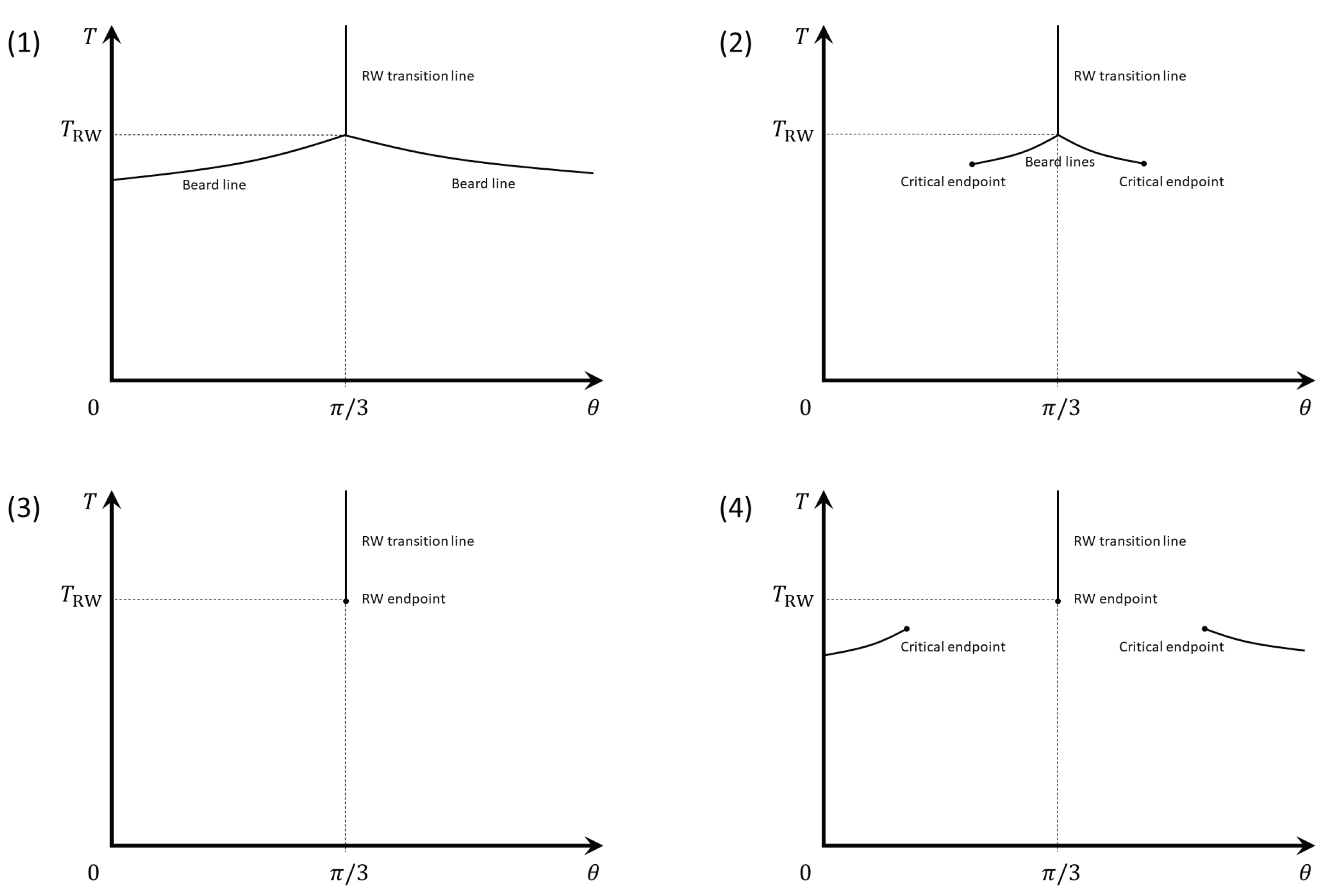
Throughout this paper, we only consider ${\mu }_{\mathrm{R}}=0$. In the thermodynamics limit, the quark number density should have a gap at $\theta =(2k-1)\pi /3$ with $T>T_{\mathrm{RW}}$; this is simply the RW transition. It should be noted that there is the possibility that the quark number density would have a gap near $\theta =(2k-1)\pi /3$ corresponding to points on the beard line starting from the RW endpoint. In the Fourier expansion of such a first-order singular quantity, we encounter the Gibbs phenomenon [37], which is not desirable. To control this phenomenon, extreme care must be taken; the Riesz summation is a famous example. One technical method is to consider a finite but sufficiently large system volume, and then the Gibbs phenomenon can be avoided thanks to the finite volume effect; the first-order singularity is turned into the steep change. In the lattice QCD simulation, the finite size effect always exists, and thus the above method is natural.

For a sufficiently small T, the quark number density can be approximated as the functional form

$$\begin{array}{cc}\hfill n_{\mathrm{q}}(T,\theta )& \sim i{a}_1\sin \left(3\theta \right),\hfill \end{array}$$

(9)

where $a_1\in \mathbb{R}$ is the T-dependent Fourier coefficient, and it approaches to 0 with the $T\to 0$ limit because $\theta$ can be absorbed into the temporal boundary condition of quarks [17]. It should be noted that constant terms do not exist in Equation (9) because $n_q(T,0)$ must be zero. If we increase T, higher-order oscillating modes must join to Equation (9);

$$\begin{array}{cc}\hfill n_{\mathrm{q}}(T,\theta )& =\sum _{n_{\mathrm{B}}=1}^{\infty }i{a}_{N_{\mathrm{B}}}\sin \left(3n_{\mathrm{B}}\theta \right),\hfill \end{array}$$

(10)

where all Fourier coefficients are real. If we consider several QCD effective models, we can estimate each coefficient numerically or analytically; for example, see [14,15]. However, we are interested in the qualitative properties of the canonical sectors in this study, and thus we do not need the actual functional form of the coefficients; we employ some lattice QCD predictions at a finite $\theta$ as summarized in the previous section.

Expression (9) is simply the Fourier decomposition, and thus we can employ several important pieces of knowledge obtained in the Fourier transformation to understand the canonical sectors. Then, we can understand that $a_k$ are common coefficients for ${\langle n_{\mathrm{q}}\rangle }_{\mathrm{C}}(T,3k)$ and ${\mathcal{Z}}_{\mathrm{C}}(T,3k)$ from Equation (4) if we consider the system with ${\mu }_{\mathrm{R}}=0$; ${\mathcal{Z}}_{\mathrm{C}}(T,k)\propto a_k$. Therefore, we can evaluate the canonical sectors from the behavior of $n_{\mathrm{q}}$. The important point is that we need a larger number of relevant expansion coefficients if the quark number density shows a steep change at certain $\theta$ which is induced by the first-order singularity in the thermodynamic limit. Moreover, there are contributions of k-quarks with $\left(k\mathrm{mod}3\right)=0$, but other contributions are forbidden because of the continuous RW periodicity of the quark number density in the finite-volume system. This fact may have a similarity with the following thermodynamic considerations: if we use the thermal mixed states from pure states at $T=0$ to describe the thermal system, there are only confined k-quark pure-states with $\left(k\mathrm{mod}3\right)=0$ even if we consider the deconfined phase at high T.

Let us denote n as the highest number of expansion coefficients for the quark number density, and $\delta$ is the error between the exact value of the quark number density and its expansion. It is known that the root mean square error is the convenient error estimation of the Fourier decomposition from the viewpoint of the pointwise convergence;

$$\begin{array}{cc}\hfill {\delta }_n& =\sqrt{{\int }_{-\pi /3}^{\pi /3}d\theta {|n_{\mathrm{q}}-{\tilde{n}}_{\mathrm{q}}|}^2}\ge 0,\hfill \end{array}$$

(11)

where ${\tilde{n}}_{\mathrm{q}}$ is the Fourier decomposed quark number density with fixed n. It should be noted that we here restrict the integral range to the $2\pi /3$ period because of the RW periodicity. This quantity converges with increasing n even if there is a first-order singularity. Based on the root mean square error, we can consider the following quantity:

$$\begin{array}{c}\hfill \overline{\delta }\equiv \sqrt{{\int }_{-\pi /3}^{\pi /3}d\theta {\left|n_{\mathrm{q}}\right|}^2}\sim \sqrt{{\int }_{-\pi /3}^{\pi /3}d\theta {\left|{\tilde{n}}_{\mathrm{q}}\right|}^2}\ge 0,\end{array}$$

(12)

where n is taken to be sufficiently large. From Parseval’s identity, we have

$$\begin{array}{cc}\hfill {\overline{\delta }}^2& \propto \sum _{n_{\mathrm{B}}=1}^{\infty }|a_{3n_{\mathrm{B}}}{|}^2=\frac{1}{{\mathcal{N}}^2}\sum _{n_{\mathrm{B}}=1}^{\infty }{\left|3n_{\mathrm{B}}{A}_{3n_{\mathrm{B}}}\right|}^2,\hfill \end{array}$$

(13)

with

$$\begin{array}{cc}\hfill \mathcal{N}& =V{\mathcal{Z}}_{\mathrm{GC}}(T,0),\hfill \end{array}$$

(14)

where $A_k$ are the Fourier coefficients coming from the partition function. The quantity $\overline{\delta }$ manifests

$$\begin{array}{c}\hfill \left|\sum _{n_{\mathrm{B}}=1}^{\infty }{a}_k\right|\le \overline{\delta }.\end{array}$$

(15)

Equation (13) is obtained from expressions (2) and (5) via the differential with respect to $\mu$. In quantity ${\overline{\delta }}^2$, coefficients induced from higher-order oscillating modes are enhanced by the $3n_{\mathrm{B}}$ factor, and this throws those contributions into sharp relief.

Computations of individual Fourier coefficients coming from canonical sectors are difficult, particularly for highly oscillating modes, but ${\overline{\delta }}^2$ is rather easy to compute. Equation (15) clearly shows the relation between ${\overline{\delta }}^2$ and the structure of the canonical sectors. Therefore, we can define the following quantity for each T:

$$\begin{array}{cc}\hfill d{\overline{\delta }}^2& =\frac{\partial {\overline{\delta }}^2}{\partial T},\hfill \end{array}$$

(16)

This quantity is directly related to the thermal modification of the canonical sectors. Based on the quantity, we can evaluate the canonical sectors from the behavior of the quark number density without the direct evaluation of ${\mathcal{Z}}_{\mathrm{C}}(T,Q)$. Moreover, in QCD, we can consider some other quantities such as the chiral condensate, the entropy density and so on in the evaluation of the canonical sectors, in principle. However, ${\mathcal{Z}}_{\mathrm{C}}$ depends on the current quark mass, the temperature and some other parameters except the chemical potential. Therefore, those quantities are not preferable to see the information of pure canonical sectors; the pressure is, of course, a good quantity, but the pressure is difficult to calculate precisely compared with the quark number density in the lattice QCD simulation.

Let us summarize some asymptotic behavior of ${\overline{\delta }}^2$ here. We discuss the limits of $T\to \infty$ and $m\to \infty$ as follows. The infinite T limit of ${\tilde{\delta }}^2$ can be obtained as

$$\begin{array}{c}\hfill {\overline{\delta }}^2\to {\int }_{-\pi /3}^{\pi /3}d\theta {\left|n_{\mathrm{q}}^{\mathrm{pert}.}\right|}^2,\end{array}$$

(17)

where $n_{\mathrm{q}}^{\mathrm{pert}.}$ is the quark number density obtained from the perturbative one-loop effective potential [38,39,40] as

$$\begin{array}{cc}\hfill & p^{\mathrm{pert}}.\to \frac{{\pi }^{2}i{N}_{\mathrm{c}}{N}_{\mathrm{f}}{T}^4}{3}\left[\frac{7}{60}-2{\left(\frac{\theta }{2\pi }\right)}^2+4{\left(\frac{\theta }{2\pi }\right)}^4\right],\hfill \\ \hfill & n_{\mathrm{q}}^{\mathrm{pert}.}(T,\theta )\to \frac{2\pi i{N}_{\mathrm{c}}{N}_{\mathrm{f}}{T}^3}{3}\left[\frac{\theta }{2\pi }-4{\left(\frac{\theta }{2\pi }\right)}^3\right],\hfill \end{array}$$

(18)

in the $-\pi /3\le \theta \le \pi /3$ range where p is the pressure defined as

$$\begin{array}{cc}\hfill p& =\frac{1}{\beta V}\ln {\mathcal{Z}}_{\mathrm{GC}}.\hfill \end{array}$$

(19)

Then, the quark number density can be derived from the pressure. The above expression becomes exact in the $T\to \infty$ limit; see [41] and references therein for some discussions of the Stefan–Boltzmann limit at a finite $\theta$. It should be noted that we simply estimate $\tilde{\delta }$ with the infinite T limit, and thus some more contributions must be considered when we consider realistic situations; for example, see [42]. In addition, the above potential cannot work for the whole ${\mu }_{\mathrm{R}}$ region because of the convergence restriction; for example, see [40]. Fortunately, our calculation is done with a pure imaginary $\mu$, and thus the above one-loop potential can describe the infinite T limit because the pure imaginary $\mu$ does not introduce an additional energy scale unlike the real $\mu$. In addition, we can simply discuss the infinite quark mass limit by using the hopping parameter expansion on the lattice. After the straightforward calculation, the quark number density can be expressed with the hopping parameter expansion and lattice discretization as

$$\begin{array}{c}\hfill n_{\mathrm{q}}(T,\theta )=-\frac{i{N}_{\mathrm{f}}{T}^3}{N_s^3{N}_t}\sum _{l=1}^{\infty }{\kappa }^l\langle \mathrm{Tr}\left(\frac{\partial D}{\partial \mu }{D}^{l-1}\right){\rangle }_{\mathrm{GC}},\end{array}$$

(20)

where $\kappa =1/(2m+8)$ with the quark mass m, $N_s^3{N}_t$ is the four dimensional lattice volume and D denotes the covariant derivative; see [43] for details of the expansion. Since Equation (22) is $1/m$ suppressed, ${\overline{\delta }}^2$ becomes zero in the $m\to \infty$ limit, and thus we need extreme care to determine the confinement–deconfinement transition temperature in the pure gauge limit. In this sense, ${\tilde{\delta }}^2$ is mainly responsible for the quark properties because the $n=0$ contribution in the canonical sector, which mainly contains the gluonic and mesonic contributions, disappears in $n_{\mathrm{q}}$.

Panels in Figure 1 show possible scenarios for the phase structure of QCD at a finite $\theta$ in the thermodynamic limit. The first, second and third panels are expected to be realized in the heavy quark mass regime, the moderate quark mass regime and the small quark mass regime, respectively. We here summarize what we can expect in each case.

(1)

In the case of the first panel of Figure 1, there is no second-order transition point at a finite $\theta$ with any T. However, $n_{\mathrm{q}}$ is 0 at $\mu =0$ and thus the first-order singularity cannot induce the singularity in ${\overline{\delta }}^2$. We can expect a rapidly changing point near the temperature at which the first-order transition line meets the T-axis. The temperature of the rapidly changing point approaches to $T_{\mathrm{RW}}$ with increasing quark mass. Then, the temperature is the characteristic energy scale of the confinement–deconfinement transition;

(2)

In the case of the second panel of Figure 1, there are second-order points corresponding to the endpoints of the beard lines. In this case, ${\overline{\delta }}^2$ rapidly changes around $T_{\mathrm{Beard}}$ and/or $T_{\mathrm{RW}}$, but there are no singularities. We may interpret this as the characteristic energy scale for the confinement–deconfinement transition;

(3)

In the case of the third panel of Figure 1, there are second-order points at the RW endpoints. From the same discussion as in case 2, we can observe a steep change of ${\overline{\delta }}^2$ around $T_{\mathrm{RW}}$, but there are no singularities. We may interpret this as the characteristic energy scale for the confinement–deconfinement transition;

(4)

In the case of the fourth panel of Figure 1, the first-order transition line is attached to the $\mu =0$ line, but it does not start from the RW endpoint. At present, this situation is not obtained in lattice QCD simulations and QCD effective model computations. We here present it as a possible scenario, but it seems to be unfeasible in QCD.

These observations indicate that properties of the system at a finite T with ${\mu }_{\mathrm{R}}=0$ are characterized by the phase structure at finite imaginary chemical potential; the canonical sectors represent elementary excitation modes in the system and thus structural changes of the relevant canonical sectors are important factors to understand the thermal confinement–deconfinement transition. This result is almost consistent with the results obtained in [4,5,6] and also the crossover behavior reported in several studies. In the case with ${\mu }_{\mathrm{R}}\ne 0$, Equation (6) is no longer valid, and thus we cannot proceed with our discussion straightforwardly; we keep this extension for our future work.

For the reader’s convenience, we here show the T-dependence of ${\overline{\delta }}^2$ in Figure 2 as an example by employing the Polyakov-loop extended Nambu–Jona-Lasinio (PNJL) model [44] with the same model setting used in [25]. In the following, we briefly summarize the formulation of the PNJL model.

The Lagrangian density of the two-flavor PNJL model is

$$\begin{array}{cc}\hfill {\mathcal{L}}_{\mathrm{PNJL}}=& \overline{q}(i{\gamma }_{\nu }{D}^{\nu }-m_0)q+G[{\left(\overline{q}q\right)}^2+{\left(\overline{q}i{\gamma }_5\overrightarrow{\tau }q\right)}^2]-\mathcal{U}(\Phi \left[A\right],\overline{\Phi }\left[A\right],T),\hfill \end{array}$$

(21)

where $D^{\nu }={\partial }^{\nu }+i{A}^{\nu }$, q denotes the quark field, $m_0$ is the current quark mass and $\mathcal{U}$ means the Polyakov-loop potential; here, we use the same potential proposed in [45]. The gluon field $A^{\nu }$ is defined as $A^{\nu }=g{A}_a^{\nu }\frac{{\lambda }_a}{2}$ with the gauge field $A_a^{\nu }$, the Gell–Mann matrix ${\lambda }_a$, the gauge coupling constant g and the matrix $\overrightarrow{\tau }$, which stands for the isospin matrix. The symbol G denotes the coupling constant. In the PNJL model, the gauge field $A_{\mu }$ is treated as a homogeneous static temporal background field $A_4$; $A_{\mu }={\delta }_{4\mu }{A}_4$. In the Polyakov gauge, the Polyakov loop and its conjugate, $\Phi$ and $\overline{\Phi }$, are diagonal in the color space as

$$\begin{array}{cc}\hfill \Phi & =\frac{1}{3}{\mathrm{tr}}_{\mathrm{c}}\left(L\right),\overline{\Phi }=\frac{1}{3}{\mathrm{tr}}_{\mathrm{c}}\left(\overline{L}\right),\hfill \end{array}$$

(22)

with

$$\begin{array}{cc}\hfill L& =e^{ig{A}_4/T}=\mathrm{diag}\left(e^{i{\varphi }_a/T},e^{i{\varphi }_b/T},e^{-i({\varphi }_a+{\varphi }_b)/T}\right),\hfill \end{array}$$

(23)

where ${\varphi }_a$ and ${\varphi }_b$ are represented by ${\varphi }_3$ and ${\varphi }_8$ combined with ${\lambda }_3$ and ${\lambda }_8$ like as

$$\begin{array}{c}\hfill g{A}_4={\varphi }_3{\lambda }_3+{\varphi }_8{\lambda }_8.\end{array}$$

(24)

After using the mean field approximation in Equation (21), the thermodynamic potential per unit volume can be obtained as

$$\begin{array}{cc}\hfill & {\Omega }_{\mathrm{PNJL}}=-2N_{\mathrm{f}}\int \frac{d^{3}p}{{\left(2\pi \right)}^3}[3E_p\hfill \\ \hfill & +\frac{1}{\beta }\ln [1+3(\Phi +\overline{\Phi }{e}^{-\beta (E_p-\mu )})e^{-\beta (E_p-\mu )}+e^{-3\beta (E_p-\mu )}]\hfill \\ \hfill & +\frac{1}{\beta }\ln [1+3(\overline{\Phi }+\Phi e^{-\beta (E_p+\mu )})e^{-\beta (E_p+\mu )}+e^{-3\beta (E_p+\mu )}]]\hfill \\ \hfill & +U_{\mathrm{M}}+\mathcal{U},\hfill \end{array}$$

(25)

where we fix $N_{\mathrm{f}}=2$, $\mu ={\mu }_{\mathrm{R}}+i{\mu }_{\mathrm{I}}={\mu }_{\mathrm{R}}+iT\theta$, $E_p=\sqrt{{\mathbf{p}}^2+{(m_0-2G\sigma )}^2}$ and $U_{\mathrm{M}}=G{\sigma }^2$ here $\sigma =\langle \overline{q}q\rangle$. It should be noted that the thermodynamic limit is imposed to use the mean-field approximation here, and we normalize ${\overline{\delta }}^2$ by $1/T_{\mathrm{RW}}^6$ to make it dimensionless where $T_{\mathrm{RW}}$ is about 254 MeV in the present model setting.

We can see the rapid change of ${\tilde{\delta }}^2$ in this model. From the figure, we can see that the structure of canonical sectors begins to change strongly above $T\sim 0.9$ and rapidly changes around $T/T_{\mathrm{RW}}\sim 1$; see also Figure 3 for the numerical result of $d{\overline{\delta }}^2$.

It should be noted that similar quantities of ${\overline{\delta }}^2$ have been calculated to date, such as the dual chiral condensate [46,47,48,49,50], the dual meson condensate [51] and the dual version of the pressure [52]. All of these are quantities that are obtained via the integration of the corresponding quantities by $\theta$:

$$\begin{array}{cc}\hfill {\Sigma }_{\mathcal{O}}^{\left(n\right)}(T,{\mu }_{\mathrm{R}}=0)& ={\int }_{-\pi }^{\pi }\frac{d\theta }{2\pi }{e}^{-in\theta }{\langle \mathcal{O}\rangle }_{\mathrm{GC}},\mathrm{fix}(T,\theta ),\hfill \end{array}$$

(26)

where ${\langle \mathcal{O}\rangle }_{\mathrm{GC}},\mathrm{fix}$ is the expectation value of the arbitrary operator $\mathcal{O}$ at each $\theta$ with the fixed gauge configurations at $\mu =0$. The $n=1$ component has usually been treated as the approximate order parameter of the confinement–deconfinement transition so far. Unfortunately, with the quantity (26), it is unclear how to remove the Roberge–Weiss periodicity to obtain a nonzero value for $n=1$ after the integration except the quenched calculation; there is no clear reason that we always restrict the gauge configuration to compute ${\langle \mathcal{O}\rangle }_{\mathrm{GC}},\mathrm{fix}$ at $\mu =0$. From those perspectives, ${\overline{\delta }}^2$ is the better quantity in comparison with the dual quantity (26) because ${\overline{\delta }}^2$ does not suffer from uncertainty regarding its foundation. If we change ${\overline{\delta }}^2$ to be a closer form of the dual quantity (26), the following functional form seems to be suitable:

$$\begin{array}{cc}\hfill {\Sigma }_{n_{\mathrm{q}}^2}^{\left(n\right)}(T,{\mu }_{\mathrm{R}}=0)& \equiv {\int }_{-\pi /3}^{\pi /3}\frac{d\theta }{2\pi }{e}^{-in\theta }{\left|n_{\mathrm{q}}(T,\theta )\right|}^2,\hfill \end{array}$$

(27)

where we do not need to fix the gauge configuration at $\mu =0$. In this quantity, the integration range is restricted to one period ($2\pi /3$), and thus the quantity with $n=1$ can be nonzero. This restriction of the integral range was first proposed in [25] in a different context. Interestingly, the Fourier transformation with the restriction can reproduce the full-range Fourier transformation; it holds not only for the chiral condensate but also for the Polyakov loop, which is not the RW periodic quantity [25]. Therefore, the above restriction does not lose any information regarding the thermodynamic quantities in the Fourier transformation. We verified that the same tendency appears for ${\overline{\delta }}^2$ and ${\Sigma }_{n_{\mathrm{q}}^2}^{\left(1\right)}$, at least in the present model, and thus we do not show the actual result of ${\Sigma }_{n_{\mathrm{q}}^2}^{\left(1\right)}$ here.

5. Discussion and Summary

In this study, we have investigated the QCD phase structure at a finite temperature (T) and zero real chemical potential (${\mu }_{\mathrm{R}}=0$) by using the canonical ensemble. We have constructed the canonical ensemble by using the imaginary chemical potential (${\mu }_{\mathrm{I}}$). With the relation between the quark number density and the grand canonical partition function, we can investigate the canonical sectors from the structure of the quark number density at finite $\theta$ where $\theta :={\mu }_{\mathrm{I}}/T$.

To evaluate the structure of the canonical sectors not only for lower oscillating modes but also for higher oscillating modes, we propose a new quantity which is based on the mean root squared error denoted as ${\overline{\delta }}^2$. This quantity is directly related with the sum of Fourier coefficients which have a relation with each canonical sector via Parseval’s identity known in the Fourier transformation. With this quantity, we consider the possible scenario of the thermal QCD phase structure at ${\mu }_{\mathrm{R}}=0$ and clarify the corresponding consequences. In realistic QCD, we usually encounter second-order points at a finite $\theta$ which can be expected from the state-of-art lattice QCD results, and then we can expect a rapid change of ${\overline{\delta }}^2$ near the $T_{\mathrm{RW}}$. This result perfectly matches our crossover expectation that there are no singularities in the thermodynamic quantities. Therefore, we clarify that the phase structure at a finite $\theta$ is a crucial ingredient to understand the thermal QCD phase structure at zero density. Finally, we discuss the relation between the dual chiral condensate and ${\overline{\delta }}^2$.

We here summarize the advantages of the present $\tilde{\delta }$. First, this quantity reflects the changes of the canonical sectors at finite T. Particularly, it can represent the effects induced by higher-order modes of the canonical sectors; those higher-order modes may have information about the deconfined state. Second, $\tilde{\delta }$ can be easily calculated in comparison with the canonical partition function itself, even in lattice QCD simulation. Third, $\tilde{\delta }$ is constructed from the quark number density which is not directly related to the ${\mathbb{Z}}_{\mathrm{N}}\mathrm{c}$ symmetry unlike the Polyakov loop, and thus its relation with the deconfinement transition is interesting from the viewpoint of symmetries. We hope that $\tilde{\delta }$ sheds light on the confinement–deconfinement transition from the canonical sectors.

Unfortunately, we cannot investigate the spatial structure of the gauge configuration from the structure of the canonical sectors because our present discussions are based on the quark number density, where the spatial average is implicitly imposed. We will keep this topic for our future work. Therefore, some more investigations are required; for example, a persistent homology may be a promising tool [53,54,55,56,57]. In addition, our numerical estimation of $\tilde{\delta }$ is based on the PNJL model, which is a very simple and effective QCD model. Thus, the PNJL model may not have some important features of QCD even if it can describe some QCD properties, such as the chiral property, qualitatively; for example, see [58]. For example, the PNJL model does not have tetraquark contributions, but tetraquarks are expected to induce interesting phenomena even at zero chemical potential from the viewpoint of the chiral symmetry; for example, see [59]. These points will also be covered in our future work.

References

1. Greensite, J. An Introduction to the Confinement Problem; Springer: Heidelberg, Germany, 2011; Volume 821. [Google Scholar]
2. Detar, C.E.; McLerran, L.D. Order Parameters for the Confinement - Deconfinement Phase Transition in SU(N) Gauge Theories With Quarks. Phys. Lett. 1982, 119B, 171–173. [Google Scholar] [CrossRef]
3. Sato, M. Topological discrete algebra, ground state degeneracy, and quark confinement in QCD. Phys. Rev. 2008, D77, 045013. [Google Scholar] [CrossRef] [Green Version]
4. Kashiwa, K.; Ohnishi, A. Topological feature and phase structure of QCD at complex chemical potential. Phys. Lett. 2015, B750, 282–286. [Google Scholar] [CrossRef] [Green Version]
5. Kashiwa, K.; Ohnishi, A. Quark number holonomy and confinement-deconfinement transition. Phys. Rev. 2016, D93, 116002. [Google Scholar] [CrossRef] [Green Version]
6. Kashiwa, K.; Ohnishi, A. Topological deconfinement transition in QCD at finite isospin density. Phys. Lett. 2017, B772, 669–674. [Google Scholar] [CrossRef]
7. Alexandru, A.; Faber, M.; Horvath, I.; Liu, K.F. Lattice QCD at finite density via a new canonical approach. Phys. Rev. 2005, D72, 114513. [Google Scholar] [CrossRef] [Green Version]
8. Kratochvila, S.; de Forcrand, P. QCD at zero baryon density and the Polyakov loop paradox. Phys. Rev. 2006, D73, 114512. [Google Scholar] [CrossRef] [Green Version]
9. De Forcrand, P.; Kratochvila, S. Finite density QCD with a canonical approach. Nucl. Phys. Proc. Suppl. 2006, 153, 62–67. [Google Scholar] [CrossRef] [Green Version]
10. Fukuda, R.; Nakamura, A.; Oka, S. Canonical approach to finite density QCD with multiple precision computation. Phys. Rev. 2016, D93, 094508. [Google Scholar] [CrossRef] [Green Version]
11. Oka, S. Canonical approach - Investigation of finite density QCD phase transition. arXiv 2017, arXiv:1712.08974. [Google Scholar]
12. Kashiwa, K.; Kouno, H. Anatomy of the dense QCD matter from canonical sectors. arXiv 2021, arXiv:2103.11579. [Google Scholar]
13. Kashiwa, K.; Ohnishi, A. Investigation of confinement-deconfinement transition via probability distributions. arXiv 2017, arXiv:1712.06220. [Google Scholar]
14. Almasi, G.A.; Friman, B.; Morita, K.; Lo, P.M.; Redlich, K. Fourier coefficients of the net-baryon number density and chiral criticality. arXiv 2018, arXiv:1805.04441. [Google Scholar] [CrossRef] [Green Version]
15. Vovchenko, V.; Greiner, C.; Koch, V.; Stoecker, H. Critical point signatures in the cluster expansion in fugacities. Phys. Rev. D 2020, 101, 014015. [Google Scholar] [CrossRef] [Green Version]
16. Kashiwa, K. Imaginary Chemical Potential, NJL-Type Model and Confinement–Deconfinement Transition. Symmetry 2019, 11, 562. [Google Scholar] [CrossRef] [Green Version]
17. Roberge, A.; Weiss, N. Gauge Theories With Imaginary Chemical Potential and the Phases of QCD. Nucl.Phys. 1986, B275, 734. [Google Scholar] [CrossRef]
18. Yang, C.N.; Lee, T.D. Statistical theory of equations of state and phase transitions. I. Theory of condensation. Phys. Rev. 1952, 87, 404. [Google Scholar] [CrossRef]
19. Lee, T.D.; Yang, C.N. Statistical theory of equations of state and phase transitions. II. Lattice gas and Ising model. Phys. Rev. 1952, 87, 410. [Google Scholar] [CrossRef]
20. Boyda, D.L.; Bornyakov, V.G.; Goy, V.A.; Zakharov, V.I.; Molochkov, A.V.; Nakamura, A.; Nikolaev, A.A. Novel approach to deriving the canonical generating functional in lattice QCD at a finite chemical potential. JETP Lett. 2016, 104, 657–661. [Google Scholar] [CrossRef]
21. Bornyakov, V.G.; Boyda, D.L.; Goy, V.A.; Molochkov, A.V.; Nakamura, A.; Nikolaev, A.A.; Zakharov, V.I. New approach to canonical partition functions computation in Nf=2 lattice QCD at finite baryon density. Phys. Rev. D 2017, 95, 094506. [Google Scholar] [CrossRef] [Green Version]
22. Wakayama, M.; Bornyakov, V.G.; Boyda, D.L.; Goy, V.A.; Iida, H.; Molochkov, A.V.; Nakamura, A.; Zakharov, V.I. Lee-Yang zeros in lattice QCD for searching phase transition points. Phys. Lett. B 2019, 793, 227–233. [Google Scholar] [CrossRef]
23. Wakayama, M.; Nam, S.i.; Hosaka, A. Use of the canonical approach in effective models of QCD. Phys. Rev. D 2020, 102, 034035. [Google Scholar] [CrossRef]
24. Wakayama, M.; Hosaka, A. Search of QCD phase transition points in the canonical approach of the NJL model. Phys. Lett. B 2019, 795, 548–553. [Google Scholar] [CrossRef]
25. Kashiwa, K.; Kouno, H. Roberge-Weiss periodicity, canonical sector and modified Polyakov-loop. Phys. Rev. 2019, D100, 094023. [Google Scholar] [CrossRef] [Green Version]
26. Ghoroku, K.; Kashiwa, K.; Nakano, Y.; Tachibana, M.; Toyoda, F. Extension to imaginary chemical potential in a holographic model. Phys. Rev. D 2020, 102, 046003. [Google Scholar] [CrossRef]
27. Kashiwa, K.; Sasaki, T.; Kouno, H.; Yahiro, M. Two-color QCD at imaginary chemical potential and its impact on real chemical potential. Phys. Rev. 2013, D87, 016015. [Google Scholar] [CrossRef] [Green Version]
28. Shimizu, H.; Yonekura, K. Anomaly constraints on deconfinement and chiral phase transition. Phys. Rev. 2018, D97, 105011. [Google Scholar] [CrossRef] [Green Version]
29. Kikuchi, Y. ’t Hooft Anomaly, Global Inconsistency, and Some of Their Applications. Ph.D. Thesis, Kyoto University, Kyoto, Japan, 2018. [Google Scholar]
30. Nishimura, H.; Tanizaki, Y. High-temperature domain walls of QCD with imaginary chemical potentials. arXiv 2019, arXiv:1903.04014. [Google Scholar] [CrossRef] [Green Version]
31. Weiss, N. How to Distinguish a Confining From a Deconfining Phase in Gauge Theories With Fermions. Phys. Rev. 1987, D35, 2495–2500. [Google Scholar] [CrossRef]
32. D’Elia, M.; Sanfilippo, F. The Order of the Roberge-Weiss endpoint (finite size transition) in QCD. Phys. Rev. D 2009, 80, 111501. [Google Scholar] [CrossRef] [Green Version]
33. Bonati, C.; Cossu, G.; D’Elia, M.; Sanfilippo, F. The Roberge-Weiss endpoint in Nf=2 QCD. Phys. Rev. 2011, D83, 054505. [Google Scholar]
34. Bonati, C.; de Forcrand, P.; D’Elia, M.; Philipsen, O.; Sanfilippo, F. Chiral phase transition in two-flavor QCD from an imaginary chemical potential. Phys. Rev. 2014, D90, 074030. [Google Scholar] [CrossRef] [Green Version]
35. Kashiwa, K.; Yahiro, M.; Kouno, H.; Matsuzaki, M.; Sakai, Y. Correlations among discontinuities in the QCD phase diagram. J. Phys. 2009, G36, 105001. [Google Scholar] [CrossRef] [Green Version]
36. De Forcrand, P.; Philipsen, O. The QCD phase diagram for small densities from imaginary chemical potential. Nucl. Phys. 2002, B642, 290–306. [Google Scholar] [CrossRef] [Green Version]
37. Gibbs, J.W. Fourier’s series. Nature 1898, 59, 200. [Google Scholar] [CrossRef]
38. Weiss, N. The Effective Potential for the Order Parameter of Gauge Theories at Finite Temperature. Phys. Rev. 1981, D24, 475. [Google Scholar] [CrossRef]
39. Gross, D.J.; Pisarski, R.D.; Yaffe, L.G. QCD and Instantons at Finite Temperature. Rev. Mod. Phys. 1981, 53, 43. [Google Scholar] [CrossRef]
40. Meisinger, P.N.; Ogilvie, M.C. Complete high temperature expansions for one loop finite temperature effects. Phys. Rev. D 2002, 65, 056013. [Google Scholar] [CrossRef] [Green Version]
41. Kashiwa, K.; Pisarski, R.D. Roberge-Weiss transition and ’t Hooft loops. Phys. Rev. 2013, D87, 096009. [Google Scholar] [CrossRef] [Green Version]
42. Ghiglieri, J.; Kurkela, A.; Strickland, M.; Vuorinen, A. Perturbative Thermal QCD: Formalism and Applications. Phys. Rept. 2020, 880, 1–73. [Google Scholar] [CrossRef]
43. Aarts, G.; Seiler, E.; Sexty, D.; Stamatescu, I.O. Simulating QCD at nonzero baryon density to all orders in the hopping parameter expansion. Phys. Rev. 2014, D90, 114505. [Google Scholar] [CrossRef] [Green Version]
44. Fukushima, K. Chiral effective model with the Polyakov loop. Phys. Lett. 2004, B591, 277–284. [Google Scholar] [CrossRef] [Green Version]
45. Roessner, S.; Ratti, C.; Weise, W. Polyakov loop, diquarks and the two-flavour phase diagram. Phys. Rev. 2007, D75, 034007. [Google Scholar]
46. Bilgici, E.; Bruckmann, F.; Gattringer, C.; Hagen, C. Dual quark condensate and dressed Polyakov loops. Phys. Rev. 2008, D77, 094007. [Google Scholar] [CrossRef] [Green Version]
47. Fischer, C.S. Deconfinement phase transition and the quark condensate. Phys. Rev. Lett. 2009, 103, 052003. [Google Scholar] [CrossRef] [PubMed] [Green Version]
48. Kashiwa, K.; Kouno, H.; Yahiro, M. Dual quark condensate in the Polyakov-loop extended NJL model. Phys. Rev. 2009, D80, 117901. [Google Scholar]
49. Benič, S. Physical interpretation of the dressed Polyakov loop in the Nambu–Jona-Lasinio model. Phys. Rev. 2013, D88, 077501. [Google Scholar] [CrossRef] [Green Version]
50. Xu, F.; Mao, H.; Mukherjee, T.K.; Huang, M. Dressed Polyakov loop and flavor dependent phase transitions. Phys. Rev. 2011, D84, 074009. [Google Scholar] [CrossRef] [Green Version]
51. Zhang, Z.; Wang, Y.; Lu, H. Dual meson condensates in the Polyakov-loop enhanced linear sigma model. Phys. Rev. D 2021, 103, 034017. [Google Scholar] [CrossRef]
52. Kashiwa, K. Implications of imaginary chemical potential for model building of QCD. arXiv 2016, arXiv:1603.04958. [Google Scholar]
53. Nakamura, T.; Hiraoka, Y.; Hirata, A.; Escolar, E.G.; Nishiura, Y. Persistent homology and many-body atomic structure for medium-range order in the glass. Nanotechnology 2015, 26, 304001. [Google Scholar] [CrossRef] [Green Version]
54. Hiraoka, Y.; Nakamura, T.; Hirata, A.; Escolar, E.G.; Matsue, K.; Nishiura, Y. Hierarchical structures of amorphous solids characterized by persistent homology. Proc. Natl. Acad. Sci. USA 2016, 113, 7035–7040. [Google Scholar] [CrossRef] [PubMed] [Green Version]
55. Donato, I.; Gori, M.; Pettini, M.; Petri, G.; De Nigris, S.; Franzosi, R.; Vaccarino, F. Persistent homology analysis of phase transitions. Phys. Rev. E 2016, 93, 052138. [Google Scholar] [CrossRef] [PubMed] [Green Version]
56. Hirakida, T.; Kashiwa, K.; Sugano, J.; Takahashi, J.; Kouno, H.; Yahiro, M. Persistent homology analysis of deconfinement transition in effective Polyakov-line model. Int. J. Mod. Phys. A 2020, 35, 2050049. [Google Scholar] [CrossRef]
57. Kashiwa, K.; Hirakida, T.; Kouno, H. Persistent homology analysis for dense QCD effective model with heavy quarks. arXiv 2021, arXiv:2103.12554. [Google Scholar]
58. Fukushima, K.; Skokov, V. Polyakov loop modeling for hot QCD. Prog. Part. Nucl. Phys. 2017, 96, 154–199. [Google Scholar] [CrossRef] [Green Version]
59. Pisarski, R.D.; Skokov, V.V. How tetraquarks can generate a second chiral phase transition. Phys. Rev. D 2016, 94, 054008. [Google Scholar] [CrossRef] [Green Version]
Figure 1. The schematic figures of the QCD phase diagram on the θ -T plane in the thermodynamic limit. Solid lines represent the first-order phase transition lines and closed circles mean the second-order points. We here assume that the thermodynamic quantities have a singularity only once along the T axis and T RW > T beard . Furthermore, the transition temperature is decreased with decreasing θ from θ = π / 3 0 .
Symmetry 13 01273 g001
Figure 2. The T-dependence of δ ¯ 2 at μ R = 0 is calculated by using the PNJL model. In the panel, δ ¯ 2 is normalized by 1 / T RW 6 .
Symmetry 13 01273 g002
Figure 3. The T-dependence of d δ ¯ 2 at μ R = 0 is calculated by using the PNJL model. In the panel, d δ ¯ 2 is normalized by 1 / T RW 5 .
Symmetry 13 01273 g003
Publisher’s Note: MDPI stays neutral with regard to jurisdictional claims in published maps and institutional affiliations.