Abstract
In this work, we obtain exact solutions and continuous numerical approximations for mixed problems of coupled systems of diffusion equations with delay. Using the method of separation of variables, and based on an explicit expression for the solution of the separated vector initial-value delay problem, we obtain exact infinite series solutions that can be truncated to provide analytical–numerical solutions with prescribed accuracy in bounded domains. Although usually implicit in particular applications, the method of separation of variables is deeply correlated with symmetry ideas.
1. Introduction
In real-world problems, there are time lags between actions and responses. When these time delays are much shorter than the scale of observation, and they do not significantly affect the dynamics of the system, these problems might be satisfactorily modeled using ordinary or partial differential equations (PDEs). However, there are many situations where the presence of delays can not be safely ignored, requiring the use of modeling tools such as delay differential equations (DDEs) and partial delay differential equations (PDDEs) [1,2], including, among others, problems in life sciences [3], population dynamics [4], and control engineering [5].
For transport phenomena, diffusion, and heat conduction problems, it has been long pointed out that classical models, derived from Fourier or Fick laws and resulting in parabolic partial differential equations, implied infinite speed of propagation [6,7,8,9], and alternative models including the presence of delays have been proposed, finding increasing interest and wider areas of applications in recent years (see [10,11] and references therein).
Exact and analytical–numerical solutions for the generalized diffusion equation with delay, where a delay term is added to the classical model, have been previously obtained [12,13]. In the present work, we consider coupled systems of generalized diffusion equations with delay, written in matrix form as
where ; is the delay; and the coefficient matrices A, are, in general, not simultaneously diagonalizable. We consider mixed problems for these systems, with initial condition
and boundary conditions
Exact solutions in the form of infinite series for linear constant coefficients PDEs can be obtained using the method of separation of variables (MSV). Application of the MSV to particular problems is usually straightforward, without explicit symmetry ideas, but the MSV itself, and the properties of special functions appearing in the solutions of some problems, are deeply correlated with symmetry concepts (see, e.g., [14]).
Truncating the exact infinite series solutions, obtained by applying the MSV, up to a certain term can provide continuous numerical solutions satisfying a-priori error bounds in bounded domains. The use of these approaches has proven to be useful for more general PDEs, including time-dependent PDEs [15,16], strongly coupled problems [17], and also for different types of PDDEs [12,13,18,19,20,21,22].
In the case of PDDEs, application of the MSV results in initial-value problems for DDEs, and explicit constructive solutions for these problems are required in order to derive computable analytical–numerical solutions satisfying accuracy prescriptions. One key point in the problem considered in this work is being able to obtain closed form constructive solutions of the separated vector delay problem without requiring commutativity of the matrix coefficients. A result of this type will be obtained in the next section, and, as will be indicated in the final section, it could also pave the way to address different related problems.
The structure of this paper is as follows. In the next section, an explicit expression for the initial-value vector delay problem resulting from the application of the MSV to (1)–(3) is obtained. In Section 4, a formal series solution of problems (1)–(3), resulting from the application of the MSV, is proved to be an exact classical solution of this problem under certain regularity conditions on the initial function . Next, in Section 4, bounds on the approximation errors from truncating the infinite series solution to a finite number of terms are given, allowing the construction of continuous numerical solutions with prescribed accuracy in bounded domains. In the final section, the results are summarized and discussed.
2. Separated Initial-Value Vector Delay Differential Problem
We apply the MSV to problem (1)–(3) by writing , where and . Thus, we are led to two separated problems, the spatial scalar boundary problem
with solutions , corresponding to the sequence of eigenvalues ; and the corresponding temporal initial-value vector delay differential problems
where are the Fourier coefficients in the expansion of the initial function in terms of the eigenfunctions , i.e.,
so that
We consider first the auxiliary matrix problem
where and I is the identity matrix, whose solution is given in the next lemma.
Lemma 1.
Proof.
It is clear that is a well-defined continuous function, as in each interval it is a sum of continuous functions, and values at the ends of the intervals agree. It is also immediate to check that the matrix functions defined in (15) satisfy
Thus, for , one has
Moreover, for , with , one has
□
The next lemma gives an expression for the solution of problem (11) and (12) in terms of the function defined in Lemma 1.
Lemma 2.
Consider problem (11) and (12) with and invertible. For a differentiable initial function , its solution is given by , for , and, for and , by
Proof.
A more explicit expression for the solution is presented in the next theorem.
Theorem 1.
The solution of problem (11) and (12), with conditions as in Lemma 2, is given by for , and, for and , by
where the second summation is assumed to be empty for .
Proof.
It is immediate by substituting in (21) the expression of given in (17), taking into account that , and cancelling out some terms. □
Remark 1.
Although the matrix functions have been defined in (15) recursively, they can be written explicitly as iterated integrals,
When and commute, it is not difficult to check that they are given by the following compact expression without integrals,
In particular, if and are diagonal, or with the appropriate change of variables when they are simultaneously diagonalizable, problems (11) and (12) consist of M independent scalar problems, and it can be checked that the expressions given by Theorem 1 for each component of agree with those given in [12,13] for the corresponding scalar problems.
Remark 2.
In scalar problems, diffusion coefficients are always positive, so it is common to assume in diffusion vector problems that the corresponding matrix coefficients are positive defined (see, e.g., [23]). In the next sections, where exact and numerical solutions for the coupled diffusion problems (1) and (3) are derived, we will assume the weaker condition of A being positive stable, i.e., having eigenvalues with positive real part, similar to the condition assumed in [16] for diffusion problems without delay. In this section, in Lemma 2 and Theorem 1, we have only required A to be invertible, and similarly for , or equivalently , which would be the coefficient when . As will be indicated in the last section, the solution of (11) and (12) given in Theorem 1 might find application in different problems, not necessarily of diffusion type, so that only conditions guaranteeing the obtention of compact, closed form solutions of (11) and (12) have been assumed.
When A is singular, matrices can still be defined, by replacing the definition of in (15) with the nonintegrated form
However, even in the much simpler case of commuting coefficients, infinite sums seem unavoidable, as the expression corresponding to (25) would be
3. Exact Infinite Series Solution
The solution of the general initial-value vector DDE problem given in Theorem 1 provides expressions for the functions in (10), by taking in (11) and (12) , , and . The corresponding functions for each of these problems will be denoted . Writing , the candidate series solution of problem (1)–(3) for can be written as
where
In the next theorem, we show that under a condition on the eigenvalues of A and for sufficiently regular initial functions, the three series in (29)–(31) converge uniformly and can be differentiated termwise with respect to t and twice with respect to x, and the candidate series (29) is a classical solution of problem (1)–(3). Specifically, we will assume the following conditions on the initial function :
Theorem 2.
Consider problem (1)–(3). Assume that every eigenvalue of A has positive real part, and that is invertible, where and I is the identity matrix. For any initial function satisfying the conditions given in (32), the function defined in (29) is continuous in , its derivatives and are continuous in , and it is an exact solution of problem (1)–(3).
Before proving this theorem, we present in the next lemmas bounds for the norms of matrix exponentials and of the functions . In what follows, denotes a vector norm or a compatible norm for matrices, and we will assume that the conditions of Theorem 2 hold.
Lemma 3.
For a matrix , let be the set of its eigenvalues, and . Then, for each , we can find a constant such that
Proof.
Consider the Jordan decomposition , so that , where D is diagonal, with eigenvalues of , and E is an upper triangular nilpotent matrix. Letting , one has ([24], p. 396) that . Thus, for any , there is such that for , and we can take . □
Lemma 4.
Let and . Fix such that , and write K for a constant satisfying the condition of Lemma 3. Then, can be written in the form
where the matrices admit the bounds
Proof.
We proceed by induction on k. For , one has , and we can write , where , so that
which is of the form (35).
We can now proceed to the proof of Theorem 2. We note that the conditions (3) assumed for the initial function ensure convergence of the Fourier expansions of and .
Proof of Theorem 2.
From Lemma 2, since , it follows that for each k and any finite positive t, the functions are bounded. In addition, for each t there is N such that is decreasing for .
Consider now the series obtained by termwise differentiating , as given in (28) and (29)–(31), with respect to t. We denote this series , as it will be proved that it converges uniformly in . For each of the subseries in (29)–(31) and for each k, and letting aside some constant terms, one gets infinite series of the form
for , and of the form
for and . From the conditions assumed in (3) for the initial function , it follows the uniform converge and continuity of the series
and
for . Hence, since are bounded and decreasing for n large, it follows that converges uniformly in . It is immediate to check the continuity at the connecting intervals for . For , at it is easy to check the continuity of , but in general this is not the case for , unless a special condition is required on the initial function .
Similar arguments apply for the series resulting from termwise twice differentiating with respect to x, since they have the same form as those previously discussed for . □
4. Continuous Numerical Solutions
In this section, we will obtain bounds on the errors of continuous numerical solutions of problem (1)–(3), computed by truncating to N terms the exact series solution defined in Theorem 2.
Using the decomposition of given in (34), it is immediate that the series in (29)–(31) can be written in the form
where are the respective infinite sums in (29)–(31) corresponding to the terms . Hence, the errors resulting from approximating by using the expressions for given in (44)–(46) but computing only a finite number of terms, N, in the infinite sums are
To bound these errors, we will use bounds for derived from (35), in terms of incomplete gamma functions ([25], p. 174). Letting , from (35) it follows that
We note that, from the conditions (3) assumed for the initial function , the Fourier coefficients of and decay as , so we can find constants H and such that, for ,
Hence, writing , one has
since is decreasing with respect to v and .
Similarly, for , one has
since for .
Finally, for , one has
and with the change of variable , one gets
since and .
Therefore, we have proved the following theorem.
Theorem 3.
Consider problem (1)–(3), let be the exact series solution given in Theorem 2, and let be the approximation obtained when the infinite series’ in (44)–(46) are replaced by the corresponding partial sums with N terms. Then, for
Consequently, for any and given a prescribed a-priori error there is N such that for
Next, we present an example showing the practical feasibility of computing the numerical solutions and the error bounds given in Theorem 3. In this example, we used the infinity norm; computations were performed using Maple, and graphics were prepared using Matlab.
Example 1.
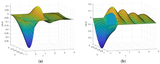
Figure 1.
Numerical solutions computed with for Example 1. (a) First component. (b) Second component.
In the next figure (Figure 2), total error bounds and individual contributions to the error bounds by the three terms in (56) are presented.
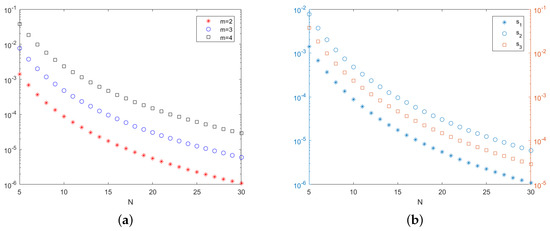
Figure 2.
Maximum error bounds (log-scale) for numerical solutions of Example 1 for , with , in terms of N. (a) Error bounds for different m values. (b) Individual contributions to total error bound, for , of the first (), second (), and third term () in (56), with different scales for the first two terms (left axis) and the third term (right axis).
In this example, the Fourier coefficients of the initial function satisfy more stringent conditions than those assumed in (51), since one has
Thus, taking , one has and . Hence, the bounds given in (56) can be refined for this example by substituting N in the denominator of the first two terms by , and in the denominator of the third term by .
For the rest of the constants in (56), it is straightforward to compute that and . Since , letting we can choose , and also, since , one gets , for .
5. Conclusions
In this work, we have presented exact and continuous numerical solutions for coupled systems of diffusion equations with delay, extending previous results for scalar problems [12,13]. These solutions are expressed in terms of the parameters of the problem, and may be used to analyze how the system behavior depends on those parameters.
As shown in Theorem 3, the analytic–numerical solutions proposed in this work may provide numerical approximations with a-priori prescribed errors in bounded domains. The error bounds given in Theorem 3 for the first two terms, and , depending on gamma incomplete functions, are essentially exponentially decaying with N; and the third term, , is . As was shown in [13], the rate of convergence can also be made exponential for this last term, by using suitable polynomial approximations to the initial function. In any case, the error bounds guaranteed by Theorem 3 are usually far from being sharp, and convergence can be much faster, especially for problems with highly regular initial functions. Additionally, when the initial function consists of a finite combination of the eigenfunctions , the exact solution defined in Theorem 2 reduces to a finite sum.
The expression given in Theorem 1 for the solution of a general initial value vector DDE problem may find applications in a wide variety of problems, beyond its use in this work. For instance, it would provide the basis to deal with related problems for coupled system with delay, as the type of reaction–diffusion equations with delay considered in [13]. More generally, since the matrix coefficients are not required to commute, this expression can be applied to obtain constructive solutions for problems involving scalar higher-order linear DDE, as they can be converted into a first-order system of the type considered in Theorem 1. The exact solution given in Theorem 1 could also provide the basis for extending previous works dealing with random scalar delay problems [26,27] to general vector delay problems, or with the construction of numerical schemes based on exact solutions [28,29,30].
Author Contributions
Conceptualization, E.R. and F.R.; methodology and formal analysis, all authors; writing—original draft preparation, F.R.; writing—review and editing, all authors. All authors have read and agreed to the published version of the manuscript.
Funding
This research was funded by Ministerio de Economía y Competitividad grant number CGL2017-89804-R.
Conflicts of Interest
The authors declare no conflict of interest. The funders had no role in the design of the study; in the collection, analyses, or interpretation of data; in the writing of the manuscript, or in the decision to publish the results.
References
- Kolmanovskii, V.; Myshkis, A. Introduction to the Theory and Applications of Functional Differential Equations; Kluwer Academic Publishers: Dordrecht, The Netherlands, 1999. [Google Scholar]
- Wu, J. Theory and Applications of Partial Functional Differential Equations; Springer: New York, NY, USA, 1996. [Google Scholar]
- Smith, H. An Introduction to Delay Differential Equations with Applications to the Life Sciences; Springer: New York, NY, USA, 2011. [Google Scholar]
- Kuang, Y. Delay Differential Equations: With Applications in Population Dynamics; Academic Press: San Diego, CA, USA, 1993. [Google Scholar]
- Wu, M.; He, Y.; She, J.-H. Stability Analysis and Robust Control of Time-Delay Systems; Science Press: Beijing, China; Springer: Berlin/Heidelberg, Germany, 2010. [Google Scholar]
- Cattaneo, C. Sur une forme de l’équation de la chaleur éliminant le paradoxe d’une propagation instantanée. C. R. Acad. Sci. 1958, 247, 431–433. [Google Scholar]
- Vernotte, P. Les paradoxes de la théorie continue de l’équation de la chaleur. C. R. Acad. Sci. 1958, 246, 3154–3155. [Google Scholar]
- Vernotte, P. Some possible complications in the phenomena of thermal conduction. C. R. Acad. Sci. 1961, 252, 2190–2191. [Google Scholar]
- Joseph, D.D.; Preziosi, L. Heat waves. Rev. Mod. Phys. 1989, 61, 41–73. [Google Scholar] [CrossRef]
- Tzou, D.Y. Macro-to Microscale Heat Transfer: The Lagging Behavior, 2nd ed.; John Wiley & Sons: Chichester, UK, 2015. [Google Scholar]
- Ghazanfarian, J.; Shomali, Z.; Abbassi, A. Macro-to Nanoscale Heat and Mass Transfer: The Lagging Behavior. Int. J. Thermophys. 2015, 36, 1416–1467. [Google Scholar] [CrossRef]
- Martín, J.A.; Rodríguez, F.; Company, R. Analytic solution of mixed problems for the generalized diffusion equation with delay. Math. Comput. Model. 2004, 40, 361–369. [Google Scholar] [CrossRef]
- Reyes, E.; Rodríguez, F.; Martín, J.A. Analytic-numerical solutions of diffusion mathematical models with delays. Comput. Math. Appl. 2008, 56, 743–753. [Google Scholar] [CrossRef]
- Miller, W. Symmetry and Separation of Variables; Cambridge University Press: Cambridge, UK, 1984. [Google Scholar]
- Jódar, L.; Almenar, P. Accurate continuous numerical solutions of time dependent mixed partial differential problems. Comput. Math. Appl. 1996, 32, 5–19. [Google Scholar] [CrossRef][Green Version]
- Jódar, L.; Navarro, E.; Martín, J.A. Exact and Analytic-Numerical Solutions of Strongly Coupled Mixed Diffusion Problems. Proc. Edinb. Math. Soc. 2000, 43, 1–25. [Google Scholar] [CrossRef]
- Almenar, P.; Jódar, L.; Martín, J.A. Mixed Problems for the Time-Dependent Telegraph Equation: Continuous Numerical Solutions with A Priori Error Bounds. Math. Comput. Model. 1997, 25, 31–44. [Google Scholar] [CrossRef]
- Scott, E.J. On a Class of Linear Partial Differential Equations with Retarded Argument in Time. Bul. Inst. Politeh. Din Iasi 1969, 15, 99–103. [Google Scholar]
- Wiener, J.; Debnath, L. Boundary value problems for the diffusion equation with piecewise continuous time delay. Int. J. Math. Math. 1997, 20, 187–195. [Google Scholar] [CrossRef]
- Khusainov, D.Y.; Ivanov, A.F.; Kovarzh, I. Solution of one heat equation with delay. Nonlinear Oscil. 2009, 12, 260. [Google Scholar] [CrossRef]
- Escolano, J.; Rodríguez, F.; Castro, M.A.; Vives, F.; Martín, J.A. Exact and analytic-numerical solutions of bidimensional lagging models of heat conduction. Math. Comput. Model. 2011, 54, 1841–1845. [Google Scholar] [CrossRef]
- Rodríguez, F.; Roales, M.; Martín, J.A. Exact solutions and numerical approximations of mixed problems for the wave equation with delay. Appl. Math. Comput. 2012, 219, 3178–3186. [Google Scholar] [CrossRef]
- Kushnir, V.P. On the Absolute Exponential Stability of Solutions of Systems of Linear Parabolic Differential Equations with One Delay. Nonlinear Oscill. 2012, 6, 50–53. [Google Scholar] [CrossRef]
- Golub, G.; Van Loan, C.F. Matrix Computations; Johns-Hopkins University Press: Baltimore, MD, USA, 1989. [Google Scholar]
- Olver, F.W.; Lozier, D.W.; Boisvert, R.F.; Clark, C.W. (Eds.) NIST Handbook of Mathematical Functions; Cambridge University Press: New York, NY, USA, 2010. [Google Scholar]
- Caraballo, T.; Cortés, J.C.; Navarro-Quiles, A. Applying the Random Variable Transformation method to solve a class of random linear differential equation with discrete delay. Appl. Math. Comput. 2019, 356, 198–218. [Google Scholar] [CrossRef]
- Calatayud, J.; Cortés, J.C.; Jornet, M. Lp-calculus approach to the random autonomous linear differential equation with discrete delay. Mediterr. J. Math. 2019, 16, 85–101. [Google Scholar] [CrossRef]
- García, M.A.; Castro, M.A.; Martín, J.A.; Rodríguez, F. Exact and nonstandard numerical schemes for linear delay differential models. Appl. Math. Comput. 2018, 338, 337–345. [Google Scholar] [CrossRef]
- García, M.A.; Castro, M.A.; Martín, J.A.; Rodríguez, F. Exact and nonstandard finite difference schemes for coupled linear delay differential systems. Mathematics 2019, 7, 1038. [Google Scholar]
- Calatayud, J.; Cortés, J.C.; Jornet, M.; Rodríguez, F. Mean Square Convergent Non-Standard Numerical Schemes for Linear Random Differential Equations with Delay. Mathematics 2020, 8, 1417. [Google Scholar] [CrossRef]


© 2020 by the authors. Licensee MDPI, Basel, Switzerland. This article is an open access article distributed under the terms and conditions of the Creative Commons Attribution (CC BY) license (http://creativecommons.org/licenses/by/4.0/).