
Local and Global Stability Analysis of Dengue Disease with Vaccination and Optimal Control


Abstract
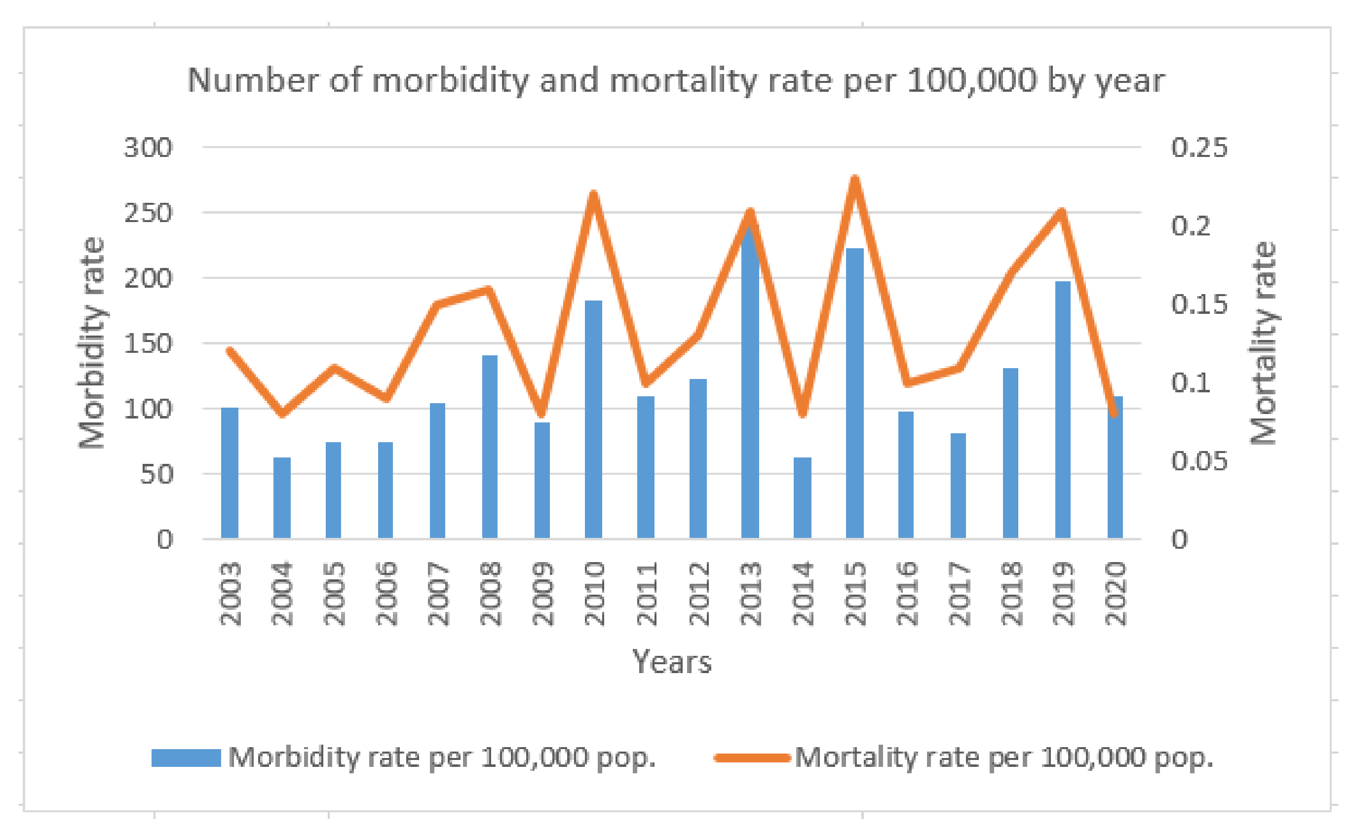
:1. Introduction
2. Materials and Methods
3. Analysis of the Model
3.1. Positivity Invariant Sets of the Model
3.2. Equilibrium Points of the Model
3.3. Basic Reproductive Number
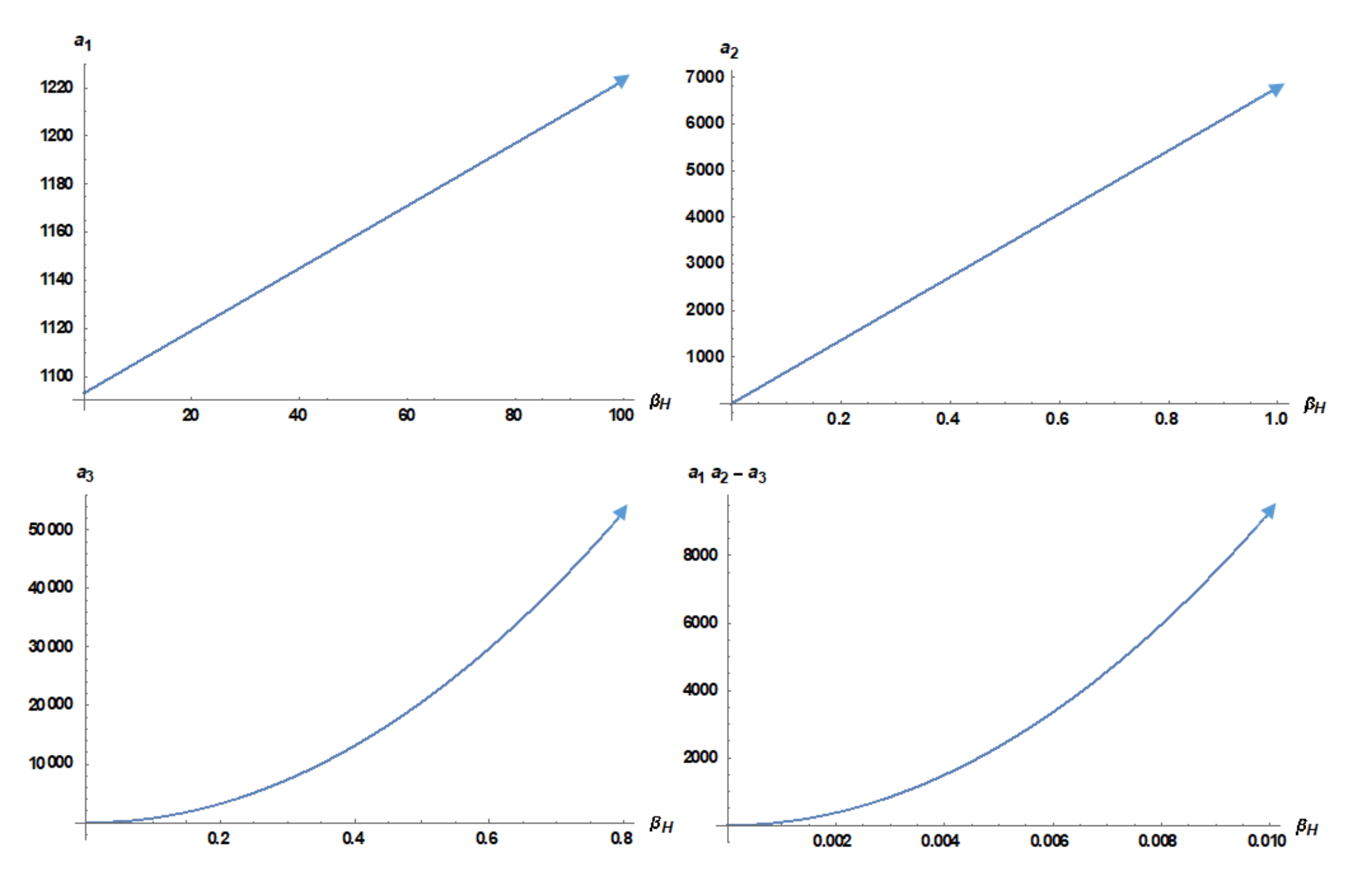
3.4. Local Stability Analysis
3.5. Global Stability Analysis
- (i)
- (ii)
- in, except at
- (iii)
- (iv)
- in, except at
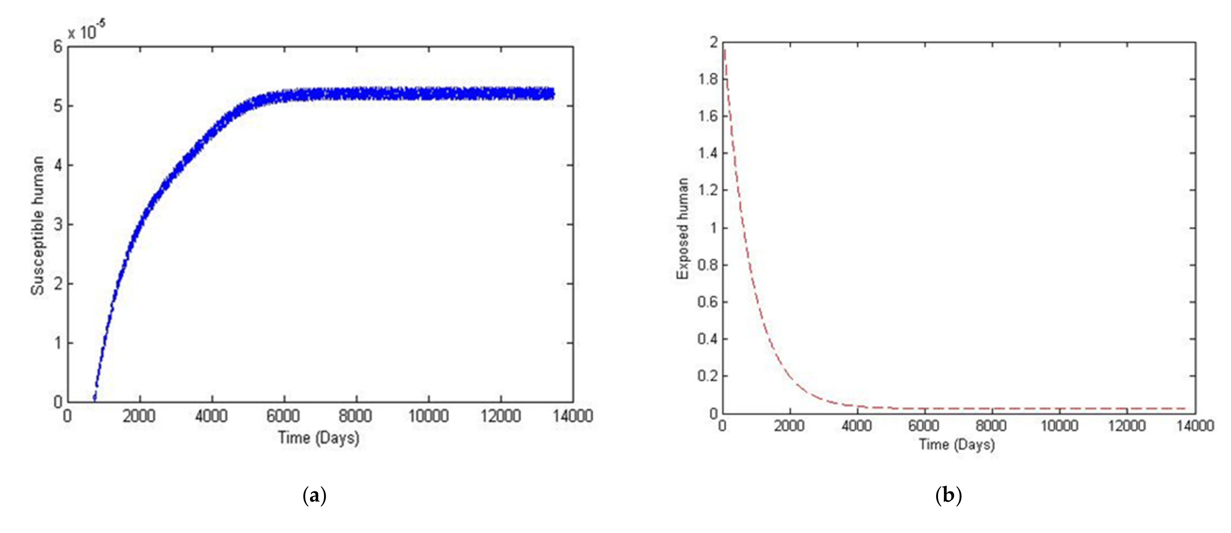
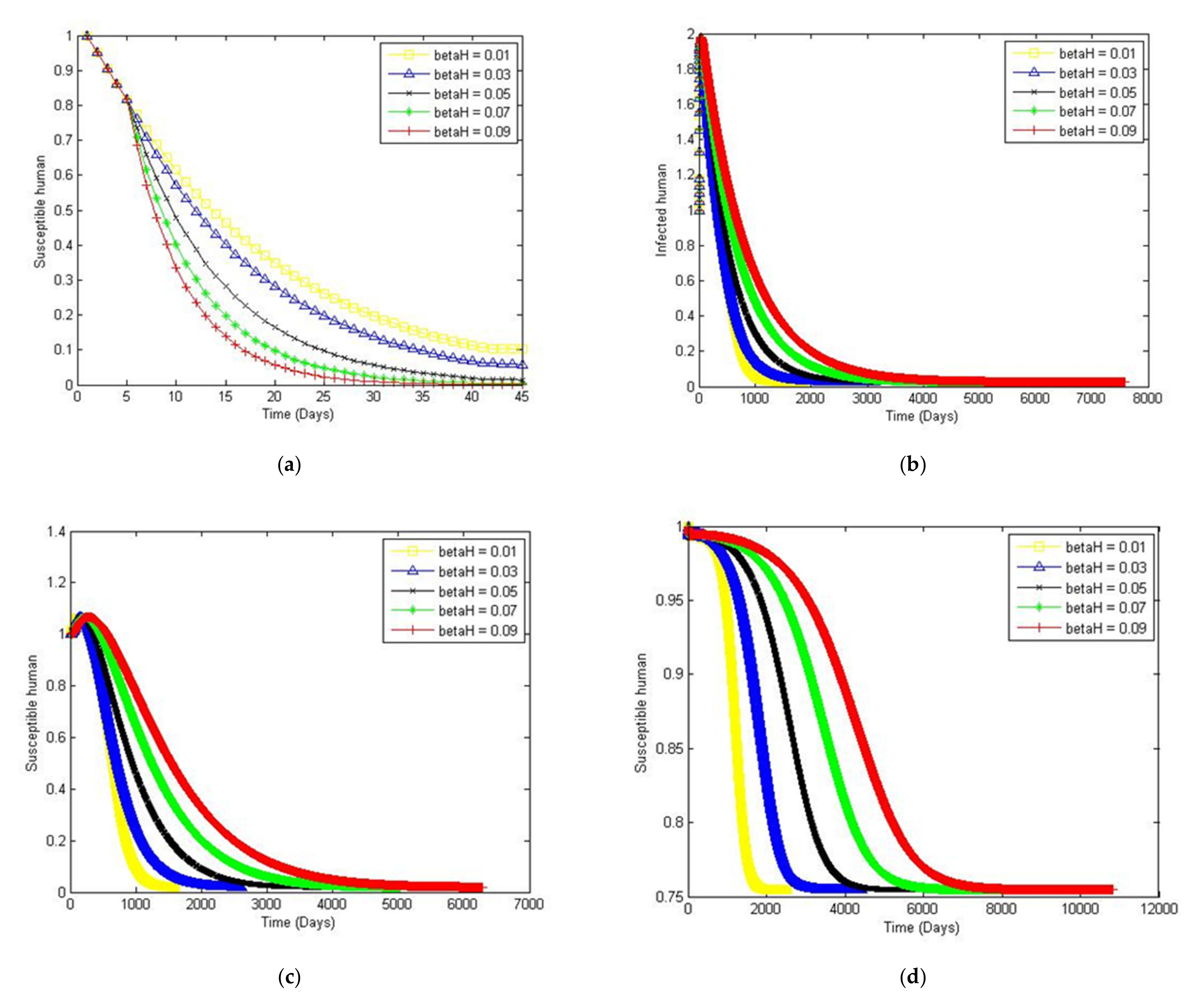
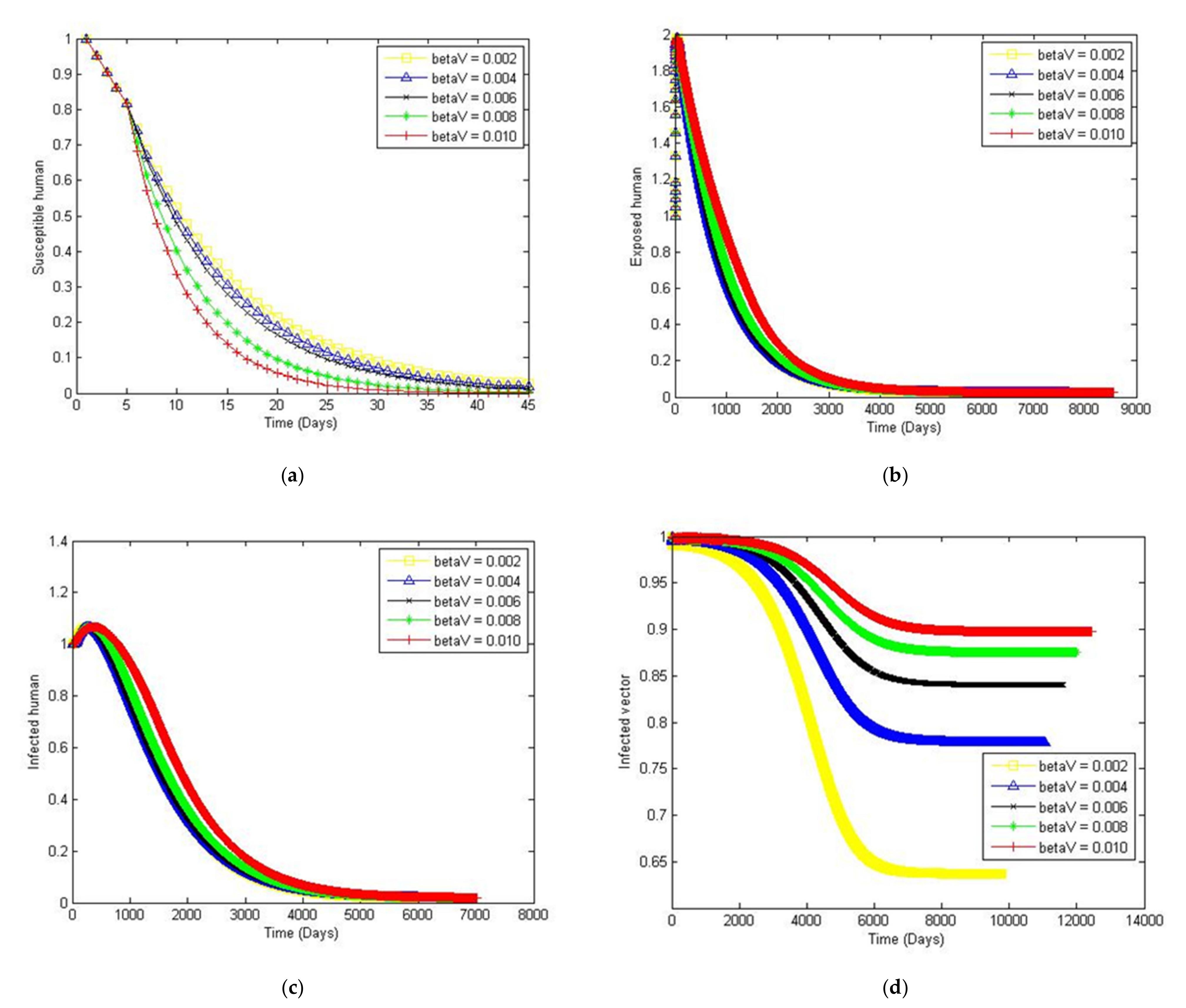
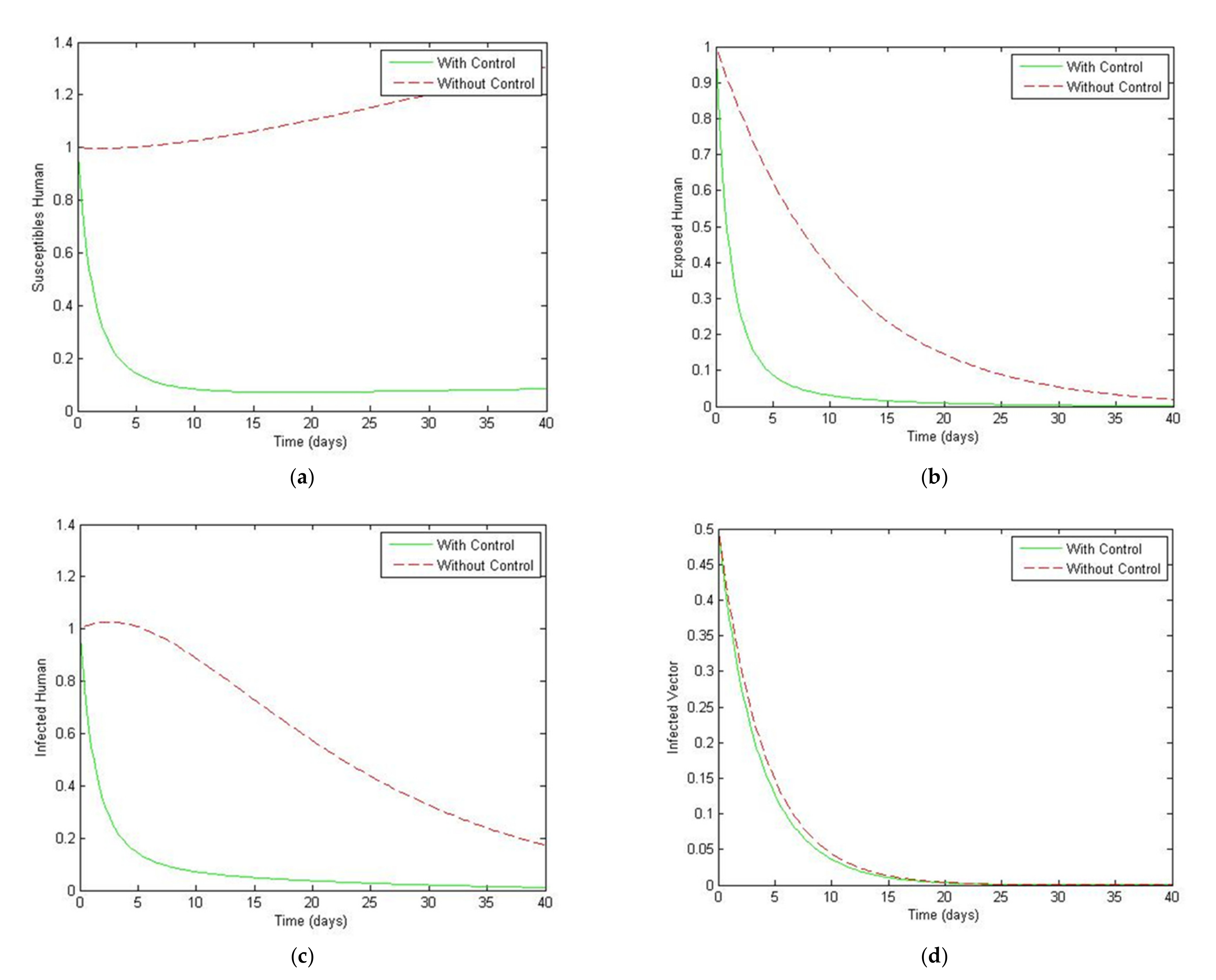
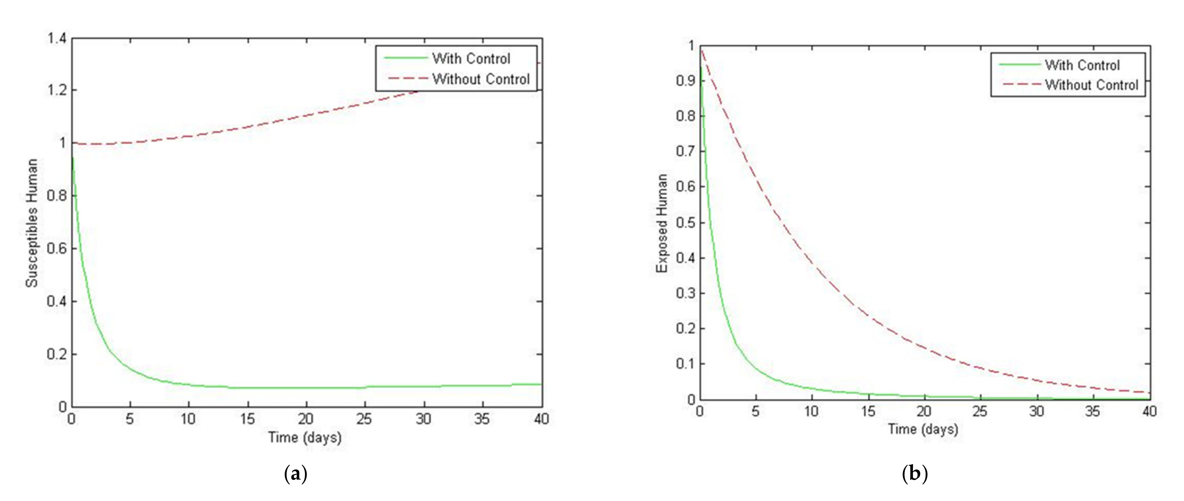
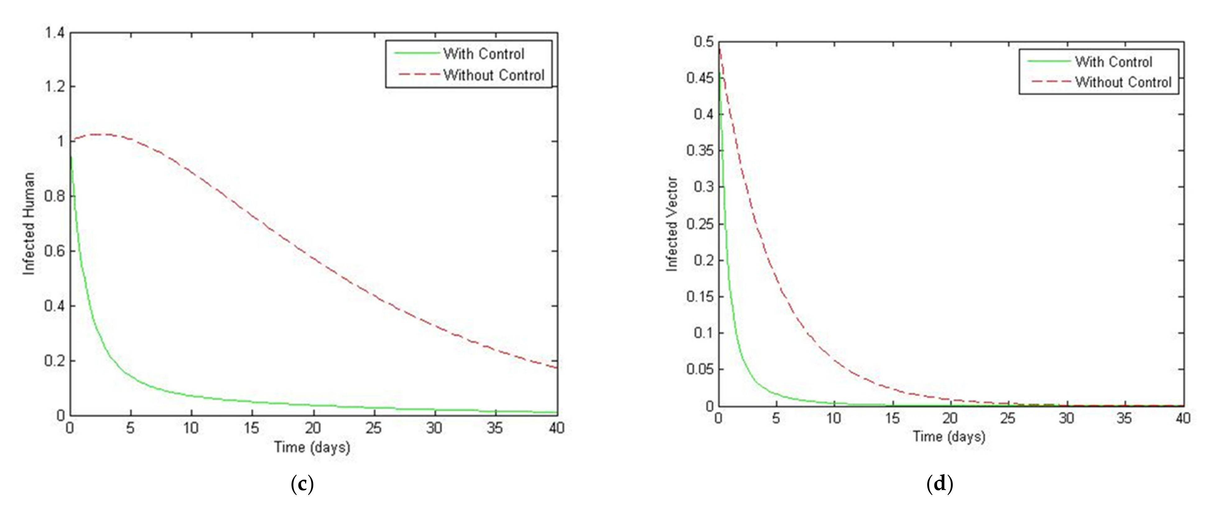
4. Numerical Simulation
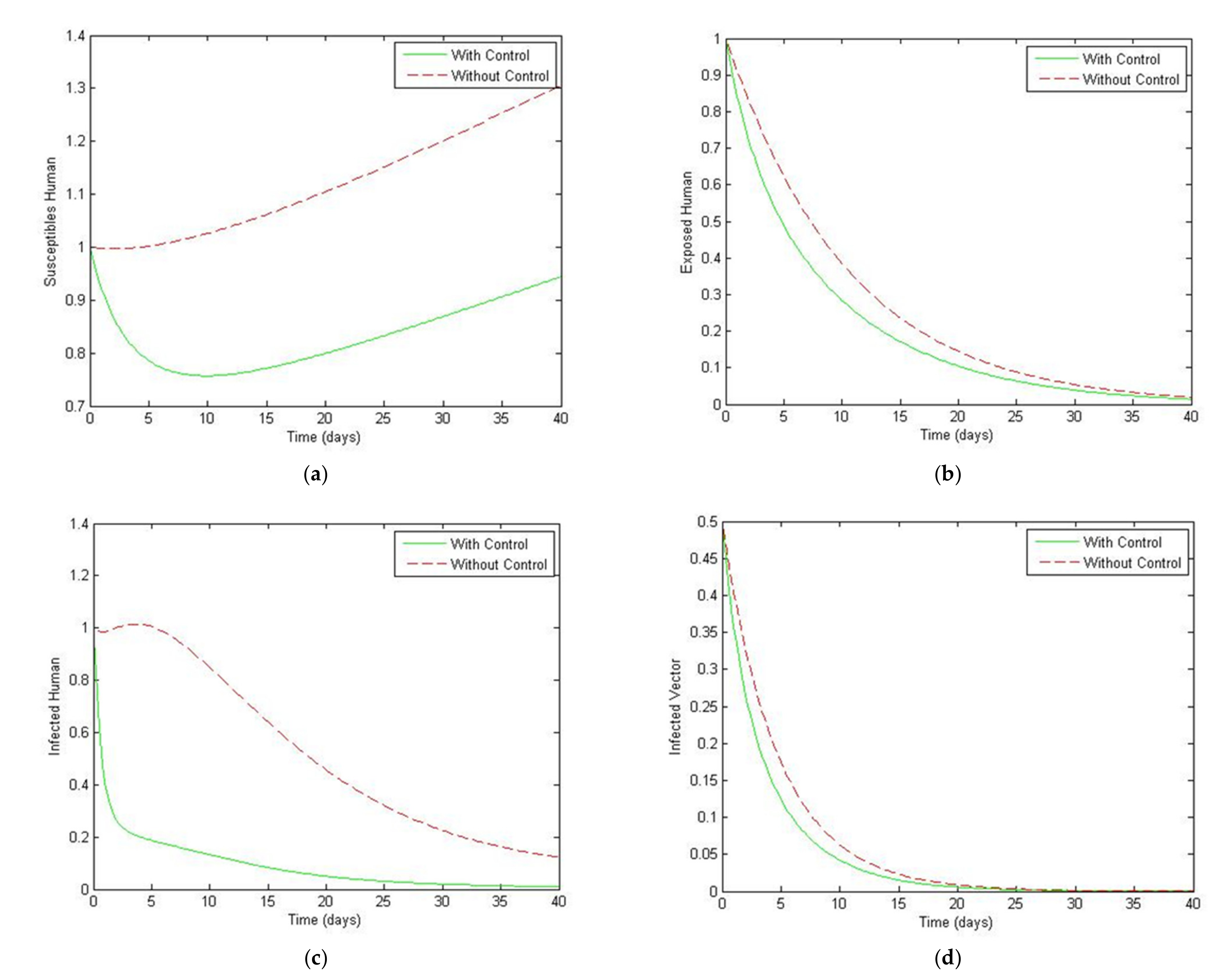
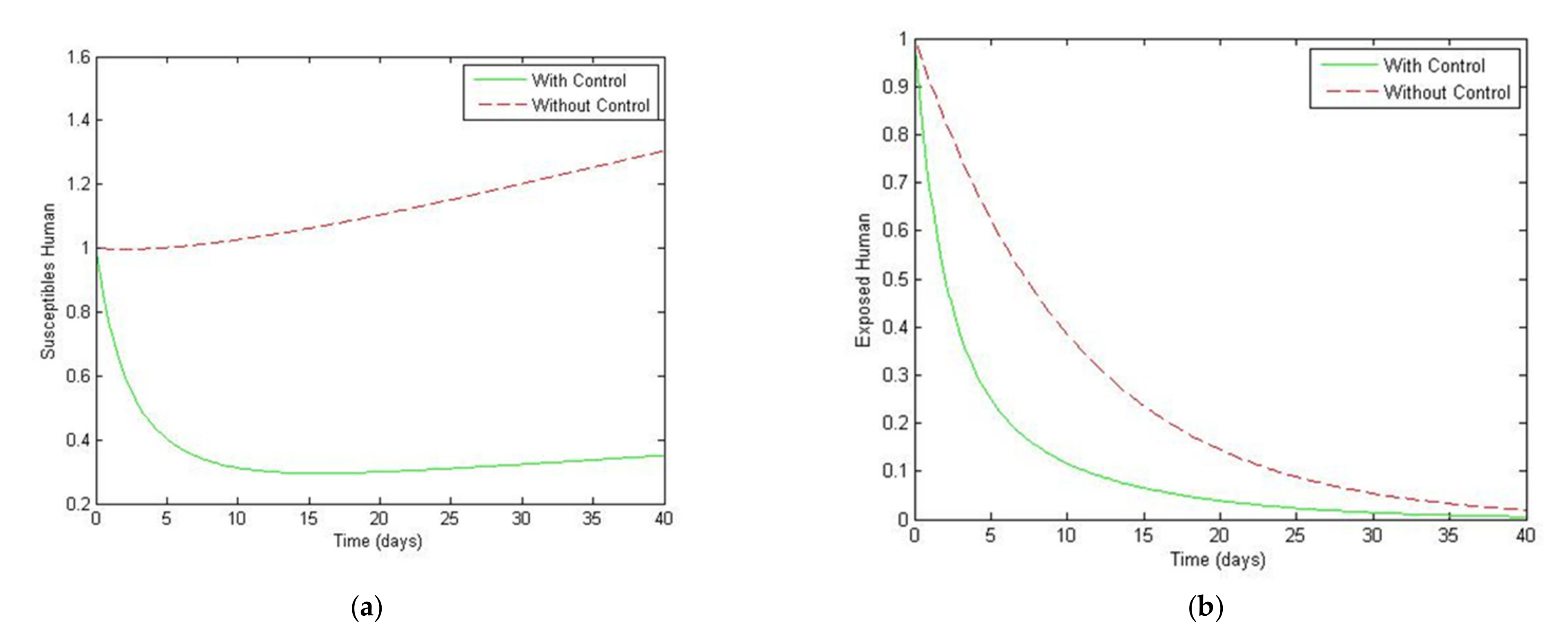
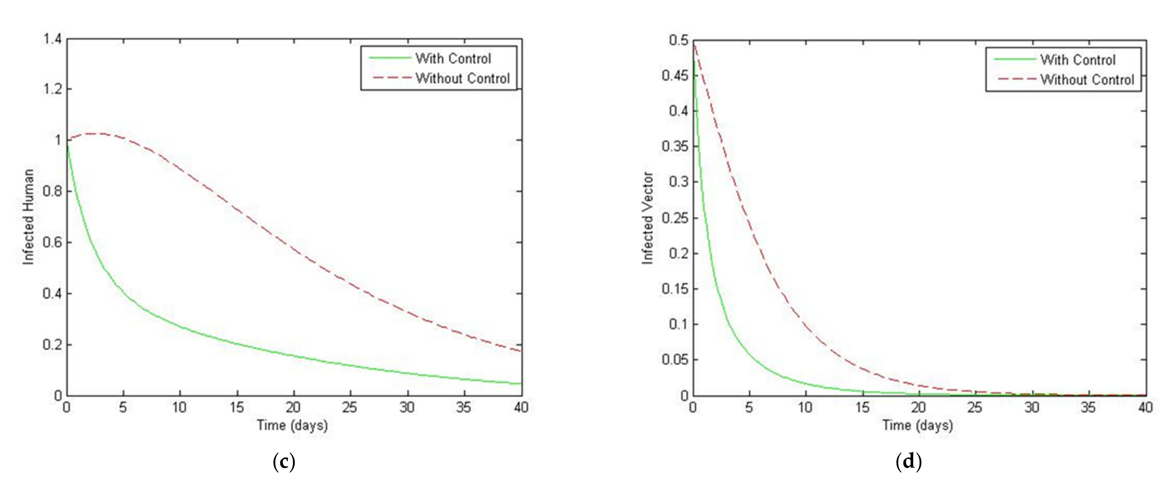
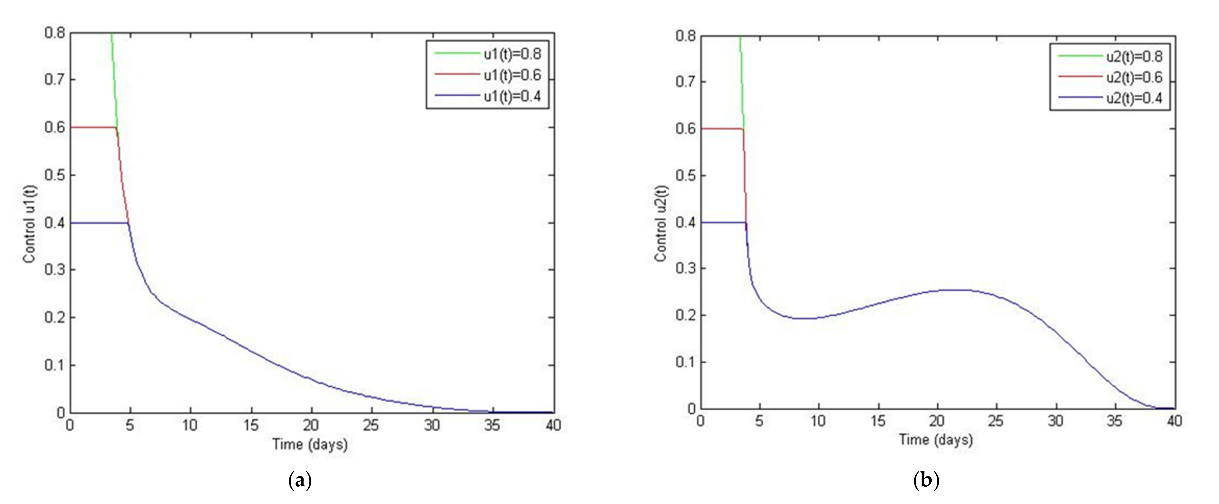
5. Optimal Control Strategies
6. Conclusions
Author Contributions
Funding
Institutional Review Board Statement
Informed Consent Statement
Data Availability Statement
Acknowledgments
Conflicts of Interest
References
- Remy, M.M. Dengue fever: Theories of immunopathogenesis and challenges for vaccination. Inflamm. Allergy Drug Targets 2014, 13, 262–274. [Google Scholar] [CrossRef]
- Ministry of Public Health, Thailand. Dengue Fever. Available online: https://ddc.moph.go.th/disease_detail.php?d=44 (accessed on 20 June 2021).
- World Health Organization. Dengue and Severe Dengue. Available online: https://www.who.int/news-room/fact-sheets/detail/dengue-and-severe-dengue (accessed on 22 January 2021).
- World Health Organization (WHO). Dengue: Guidelines for Diagnosis, Treatment, Prevention and Control: New Edition. Available online: https://apps.who.int/iris/handle/10665/44188 (accessed on 15 September 2020).
- Scott, T.W.; Amerasinghe, P.H.; Morrison, A.C.; Lorenz, L.H.; Clark, G.G.; Strickman, D.; Kittayapong, P.; Edman, J.D. Lon-gitudinal studies of aedes aegypti (Diptera: Culicidae) in Thailand and Puerto Rico: Blood feeding frequency. J. Med. Entomol. 2000, 37, 89–101. [Google Scholar] [CrossRef]
- Medlock, J.M.; Avenell, D.; Barrass, I.; Leach, S. Analysis of the potential for survival and seasonal activity of aedes albopictus (Diptera: Culicidae) in the United Kingdom. J. Vector Ecol. 2006, 31, 292–304. [Google Scholar] [CrossRef]
- World Health Organization. Updated Questions and Answers Related to the Dengue Vaccine Dengvaxia® and its Use. Available online: https://www.who.int/immunization/diseases/dengue/QA_dengue_vaccine_22Dec2017.pdf (accessed on 15 August 2021).
- World Health Organization. Comprehensive Guideline for Prevention and Control of Dengue and Dengue Haemorrhagic Fever. Revised and Expanded Edition. Available online: https://apps.who.int/iris/handle/10665/204894 (accessed on 15 August 2021).
- Kalayanarooj, S. Clinical Manifestations and Management of Dengue/DHF/DSS. Trop. Med. Health 2011, 39, S83–S87. [Google Scholar] [CrossRef] [PubMed] [Green Version]
- Gubler, D.J. Dengue and Dengue Hemorrhagic Fever. Clin. Microbiol. Rev. 1998, 11, 480–496. [Google Scholar] [CrossRef] [PubMed] [Green Version]
- Pongsumpun, P.; Tang, I. Transmission of Dengue Hemorrhagic Fever in an Age Structured Population. Math. Comput. Model. 2003, 37, 949–961. [Google Scholar] [CrossRef]
- Sriprom, M.; Pongsumpun, P.; Yoksan, S.; Barbazan, P.; Gonzalez, J.P.; Tang, I.M. Dengue haemorrhagic fever in Thailand, 1998-2003: Primary or Secondary Infection. Dengue Bull. 2003, 27, 39–45. [Google Scholar]
- Burke, D.S.; Scott, R.M.; Johnson, D.E.; Nisalak, A. A Prospective Study of Dengue Infections in Bangkok. Am. J. Trop. Med. Hyg. 1988, 38, 172–180. [Google Scholar] [CrossRef] [PubMed]
- Villar, L.; Dayan, G.H.; Arredondo-Garcia, J.L.; Rivera, D.M.; Cunha, R.; Deseda, C.; Reynales, H.; Costa, M.S.; Morales-Ramírez, J.O.; Carrasquilla, G.; et al. Efficacy of a Tetravalent Dengue Vaccine in Children in Latin America. N. Engl. J. Med. 2015, 372, 113–123. [Google Scholar] [CrossRef]
- Sabchareon, A.; Wallace, D.; Sirivichayakul, C.; Limkittikul, K.; Chanthavanich, P.; Suvannadabba, S.; Jiwariyavej, V.; Dulyachai, W.; Pengsaa, K.; Wartel, T.A.; et al. Protective efficacy of the recombinant, live-attenuated, CYD tetravalent dengue vaccine in Thai schoolchildren: A randomised, controlled phase 2b trial. Lancet 2012, 380, 1559–1567. [Google Scholar] [CrossRef]
- World Health Organization. Fact Sheet: Questions and Answers on Dengue Vaccines: Phase III Study of CYD-TDV in Latin America. Available online: http://www.who.int/immunization/research/development/QA_Dengue_vaccine_LA_phIIIstudy_final.pdf (accessed on 15 August 2021).
- Hadinegoro, S.R.; Arredondo-Garcia, J.L.; Capeding, M.R.; Deseda, C.; Chotpitayasunondh, T.; Dietze, R.; Ismail, H.H.M.; Reynales, H.; Limkittikul, K.; Rivera-Medina, D.M.; et al. Efficacy and Long-Term Safety of a Dengue Vaccine in Regions of Endemic Disease. N. Engl. J. Med. 2015, 373, 1195–1206. [Google Scholar] [CrossRef] [Green Version]
- Wilder-Smith, A. Dengue Vaccines: Dawning at last? Lancet 2014, 384, 1327–1329. [Google Scholar] [CrossRef]
- World Health Organization. Fact Sheet: Global Strategy for Dengue Prevention and Control 2012–2020. Available online: http://www.who.int/immunization/sage/meetings/2013/april/5_Dengue_SAGE_Apr2013_Global_Strategy.pdf (accessed on 5 January 2021).
- Esteva, L.; Vargas, C. Analysis of a dengue disease transmission model. Math. Biosci. 1998, 150, 131–151. [Google Scholar] [CrossRef]
- Chanprasopchai, P.; Tang, I.M.; Pongsumpun, P. SIR Model for Dengue Disease with Effect of Dengue Vaccination. Comput. Math. Methods Med. 2018, 2018, 1–14. [Google Scholar] [CrossRef] [PubMed]
- Phaijoo, G.R.; Gurung, D.B. Mathematical model of dengue fever with and without awareness in host population. Int. J. Adv. Eng. Res. Appl. 2015, 1, 239–245. [Google Scholar]
- Wu, C.; Wong, P.J.Y. Dengue transmission: Mathematical model with discrete time delays and estimation of the reproduction number. J. Biol. Dyn. 2019, 13, 1–25. [Google Scholar] [CrossRef]
- Derouich, M.; Boutayeb, A. Dengue fever: Mathematical modelling and computer simulation. Appl. Math. Comput. 2006, 177, 528–544. [Google Scholar] [CrossRef]
- Khan, M.A. Dengue infection modeling and its optimal control analysis in East Java, Indonesia. Heliyon 2021, 7, e06023. [Google Scholar] [CrossRef]
- Pongsumpun, P.; Tang, I.M.; Wongvanich, N. Optimal control of the dengue dynamical transmission with vertical transmission. Adv. Differ. Equ. 2019, 176, 1–25. [Google Scholar] [CrossRef] [Green Version]
- Chamnan, A.; Pongsumpun, P.; Tang, I.-M.; Wongvanich, N. Optimal Control of Dengue Transmission with Vaccination. Mathematics 2021, 9, 1833. [Google Scholar] [CrossRef]
- Xue, L.; Ren, X.; Magpantay, F.; Sun, W.; Zhu, H. Optimal Control of Mitigation Strategies for Dengue Virus Transmission. Bull. Math. Biol. 2021, 83, 1–28. [Google Scholar] [CrossRef] [PubMed]
- Ndaïrou, F.; Torres, D. Pontryagin Maximum Principle for Distributed-Order Fractional Systems. Mathematics 2021, 9, 1883. [Google Scholar] [CrossRef]
- Liu, G.; Chen, J.; Liang, Z.; Peng, Z.; Li, J. Dynamical Analysis and Optimal Control for a SEIR Model Based on Virus Mutation in WSNs. Mathematics 2021, 9, 929. [Google Scholar] [CrossRef]
- Ndii, M.Z.; Mage, A.R.; Messakh, J.J.; Djahi, B.S. Optimal vaccination strategy for dengue transmission in Kupang city, Indonesia. Heliyon 2020, 6, e05345. [Google Scholar] [CrossRef] [PubMed]
- Momoh, A.A.; Bala, Y.; Washachi, D.J.; Déthié, D. Mathematical analysis and optimal control interventions for sex structured syphilis model with three stages of infection and loss of immunity. Adv. Differ. Equ. 2021, 2021, 1–26. [Google Scholar] [CrossRef]
- Ministry of Public Health Thailand. Dengue Fever. Available online: http://www.boe.moph.go.th/boedb/surdata/disease.php?dcontent=old&ds=66 (accessed on 5 January 2021).
- Lamwong, J.; Wongvanich, N.; Tang, I.M.; Changpuek, T.; Pongsumpun, P. Global stability of the transmission of hand-foot-mouth disease according to the age structure of the population. Curr. Appl. Sci. Technol. 2021, 21, 351–369. [Google Scholar]
- Prathumwan, D.; Trachoo, K.; Chaiya, I. Mathematical Modeling for Prediction Dynamics of the Coronavirus Disease 2019 (COVID-19) Pandemic, Quarantine Control Measures. Symmetry 2020, 12, 1404. [Google Scholar] [CrossRef]
- Ajbar, A.; Alqahtani, R.; Boumaza, M. Dynamics of a COVID-19 Model with a Nonlinear Incidence Rate, Quarantine, Media Effects, and Number of Hospital Beds. Symmetry 2021, 13, 947. [Google Scholar] [CrossRef]
- Edelstein-Keshet, L. Mathematical Models in Biology; SIAM: New York, NY, USA, 2005. [Google Scholar]
- Basti, B.; Hammami, N.; Berrabah, I.; Nouioua, F.; Djemiat, R.; Benhamidouche, N. Stability Analysis and Existence of Solutions for a Modified SIRD Model of COVID-19 with Fractional Derivatives. Symmetry 2021, 13, 1431. [Google Scholar] [CrossRef]
- La Salle, J.; Lefschetz, S. Stability by Liapunov’s Direct Method with Applications; Academic Press: Cambridge, MA, USA, 1961. [Google Scholar]
- Rouche, N.; Habets, P.; Laloy, M. Stability Theory by Liapunov’s Direct Method; Springer: New York, NY, USA, 1977. [Google Scholar]
- Sanusi, W.; Badwi, N.; Zaki, A.; Sidjara, S.; Sari, N.; Pratama, M.I.; Side, S. Analysis and Simulation of SIRS Model for Dengue Fever Transmission in South Sulawesi, Indonesia. J. Appl. Math. 2021, 2021, 1–8. [Google Scholar] [CrossRef]
- Chien, F.; Shateyi, S. Volterra–Lyapunov Stability Analysis of the Solutions of Babesiosis Disease Model. Symmetry 2021, 13, 1272. [Google Scholar] [CrossRef]
- Shang, Y. A lie algebra approach to susceptible-infected-susceptible epidemics. Electron. J. Differ. Equ. 2012, 2012, 1–7. [Google Scholar]
- Shang, Y. Analytical Solution for an In-host Viral Infection Model with Time-inhomogeneous Rates. Acta Phys. Pol. B 2015, 46. [Google Scholar] [CrossRef] [Green Version]
- Aguiar, M.; Stollenwerk, N.; Halstead, S.B. The Impact of the Newly Licensed Dengue Vaccine in Endemic Countries. PLoS Negl. Trop. Dis. 2016, 10, e0005179. [Google Scholar] [CrossRef] [Green Version]
- Matheus, S.; Deparis, X.; Labeau, B.; Lelarge, J.; Morvan, J.; Dussart, P. Discrimination between primary and secondary dengue virus infection by an immunoglobuling avidity test using a single acute-phase serum sample. J. Clin. Microbiol. 2005, 46, 2793–2797. [Google Scholar] [CrossRef] [PubMed] [Green Version]
- Shim, E. Optimal dengue vaccination strategies of seropositive individuals. Math. Biosci. Eng. 2019, 16, 1171–1189. [Google Scholar] [CrossRef] [PubMed]
- Ndii, M.Z.; Allingham, D.; Hickson, R.; Glass, K. The effect of Wolbachia on dengue outbreaks when dengue is repeatedly introduced. Theor. Popul. Biol. 2016, 111, 9–15. [Google Scholar] [CrossRef]
- Ndii, M.Z.; Allingham, D.; Hickson, R.I.; Glass, K. The effect of Wolbachia on dengue dynamics in the presence of two serotypes of dengue: Symmetric and asymmetric epidemiological characteristics. Epidemiol. Infect. 2016, 144, 2874–2882. [Google Scholar] [CrossRef] [Green Version]
- Yang, H.M.; Macoris, M.L.G.; Galvani, K.C.; Andrighetti, M.T.M.; Wanderley, D.M.V. Assessing the effects of temperature on the population of Aedes aegypti, the vector of dengue. Epidemiol. Infect. 2009, 137, 1188–1202. [Google Scholar] [CrossRef] [Green Version]
- Lukes, D.L. Differential Equations Electronics Resource: Classical to Controlled; Academic Press: London, UK, 1982. [Google Scholar]
- Lenhart, S.; Workman, J.T. Optimal Control Applied to Biological Models; Chapman and Hall/CRC: Boca Raton, FL, USA, 2007. [Google Scholar]


| Variables and Parameters | Biological Meaning |
|---|---|
| The number of susceptible human population | |
| The number of susceptible vector population | |
| The number of exposed human population | |
| The number of infected human population | |
| The number of infected vector population | |
| The number of recovered vector population | |
| The vaccine efficiency | |
| The transmission rate of dengue virus from vector to the human | |
| The transmission rate of dengue virus from the human to vector | |
| The biting rate of vector population | |
| The recurrent infection rate | |
| The incubation rate | |
| The recovery rate | |
| The constant recruitment rate | |
| The natural mortality rate of the human population | |
| The mortality rate from infection of the human population | |
| The natural mortality rate of the vector population | |
| The mortality rate from infection of the vector population | |
| The birth rate | |
| The total number of the human population | |
| The total number of the vector population |
| Parameters | The Disease-Free | The Endemic | Source |
|---|---|---|---|
| 1/7 | 1/7 | [45,46,47,48,49,50] | |
| 1/10 | 1/10 | [45,46,47,48,49,50] | |
| 0.5 | 0.5 | [45,46,47,48,49,50] | |
| 1/(30 × 6) | 1/(30 × 6) | [45,46,47,48,49,50] | |
| 250,000 | 250,000 | estimated | |
| 200,000 | 200,000 | estimated | |
| 0.00000025 | 0.005 | assumed | |
| 0.00000012 | 0.003 | assumed | |
| 1/(365 × 70) | 1/(365 × 70) | [45,46,47,48,49,50] | |
| 1/(365 × 70) | 1/(365 × 70) | [45,46,47,48,49,50] | |
| 1/14 | 1/14 | [45,46,47,48,49,50] | |
| 1/14 | 1/14 | estimated | |
| 1/7 | 1/7 | estimated | |
| 1/14 | 1/14 | [45,46,47,48,49,50] |
Publisher’s Note: MDPI stays neutral with regard to jurisdictional claims in published maps and institutional affiliations. |
© 2021 by the authors. Licensee MDPI, Basel, Switzerland. This article is an open access article distributed under the terms and conditions of the Creative Commons Attribution (CC BY) license (https://creativecommons.org/licenses/by/4.0/).
Share and Cite
Chamnan, A.; Pongsumpun, P.; Tang, I.-M.; Wongvanich, N. Local and Global Stability Analysis of Dengue Disease with Vaccination and Optimal Control. Symmetry 2021, 13, 1917. https://doi.org/10.3390/sym13101917
Chamnan A, Pongsumpun P, Tang I-M, Wongvanich N. Local and Global Stability Analysis of Dengue Disease with Vaccination and Optimal Control. Symmetry. 2021; 13(10):1917. https://doi.org/10.3390/sym13101917
Chicago/Turabian StyleChamnan, Anusit, Puntani Pongsumpun, I-Ming Tang, and Napasool Wongvanich. 2021. "Local and Global Stability Analysis of Dengue Disease with Vaccination and Optimal Control" Symmetry 13, no. 10: 1917. https://doi.org/10.3390/sym13101917