ℒ_p-Norm-like Affine Projection Sign Algorithm for Sparse System to Ensure Robustness against Impulsive Noise

Abstract

An improved affine projection sign algorithm (APSA) was developed herein using a ${\mathcal{L}}_p$-norm-like constraint to increase the convergence rate in sparse systems. The proposed APSA is robust against impulsive noise because APSA-type algorithms are generally based on the ${\mathcal{L}}_1$-norm minimization of error signals. Moreover, the proposed algorithm can enhance the filter performance in terms of the convergence rate due to the implementation of the ${\mathcal{L}}_p$-norm-like constraint in sparse systems. Since a novel cost function of the proposed APSA was designed for maintaining the similar form of the original APSA, these have symmetric properties. According to the simulation results, the proposed APSA effectively enhances the filter performance in terms of the convergence rate of sparse system identification in the presence of impulsive noises compared to that achieved using the existing APSA-type algorithms.

1. Introduction

The adaptive filtering theory has been widely applied in several domains such as system identification, channel estimation, as well as noise and echo cancellation [1,2,3,4,5,6]. As shown in Figure 1, the main purpose of an adaptive filter is to accomplish the precise estimation of filter coefficients to minimize error signals with the same input signals. Representative adaptive filtering algorithms include the least-mean-squares (LMS) algorithm and normalized LMS algorithm, which have a low computational complexity and can be easily implemented. In addition, the affine projection algorithm (APA) [7,8,9] has been developed to enhance the convergence performance associated with correlated input signals. However, because LMS-type and APA-type algorithms are based on the ${\mathcal{L}}_2$-norm optimization of error signals, their performance deteriorates in the presence of system output noise, which includes impulsive noise.

To ensure satisfactory filter performance even in the presence of impulsive noise, several adaptive filtering algorithms derived from ${\mathcal{L}}_1$-norm optimization have recently been proposed [10,11,12,13]. A representative algorithm that is robust against impulsive noises is the affine projection sign algorithm (APSA) [11]. However, the APSA is not particularly useful in sparse system identification as network echo cancellation or underwater acoustic channel estimation, in which the impulse response is primarily composed of near-zero coefficients and only a few large coefficients. In this context, many adaptive filters have been proposed to optimize filter performance by considering the system sparsity [12,13,14,15,16,17]. Among such frameworks, adaptive filtering algorithms based on the concept of an ${\mathcal{L}}_0$-norm constraint have been considered to enhance the convergence rate of sparse systems [13,14]. In accordance with the ${\mathcal{L}}_0$-norm constraint, a ${\mathcal{L}}_p$-norm-like concept has been introduced to enhance the filter performance of LMS-type algorithms [18,19,20] and it has been demonstrated that the ${\mathcal{L}}_p$-norm-like concept can contribute to the performance enhancement of adaptive filters in sparse systems. However, due to the inherent characteristics of LMS-type algorithms, their performance remains unsatisfactory in cases involving impulsive noise.

Considering these aspects, this paper reports on an improved APSA for sparse system identification. The algorithm is based on a novel cost function derived from ${\mathcal{L}}_1$-norm optimization including the ${\mathcal{L}}_p$-norm-like constraint. Unlike the original APSA, the proposed cost function uses the a priori error instead of the a posteriori error. Consequently, the proposed APSA does not employ the approximation of the a posteriori error with the a priori error while formulating the equation to update the filter coefficient vectors. The performance of the proposed APSA in a general sparse system was evaluated and compared with those of the APSA [11], real-coefficient proportionate APSA (RP-APSA) [12], real-coefficient improved proportionate APSA (RIP-APSA) [12] and ${\mathcal{L}}_0$-APSA [13].

This paper is organized as follows. In the following Section 2, the original APSA is described. In Section 3, the proposed ${\mathcal{L}}_p$-norm-like APSA is explained in detail. In Section 4, we present the simulation results to verify the performance of the proposed APSA. Finally, Section 5 gives the conclusions of this paper.

2. Original APSA

The data vector ${\mathbf{d}}_i$ from an unknown target system is defined as

$$d_i={\mathbf{u}}_i^T{\mathbf{w}}_o+v_i,$$

(1)

where ${\mathbf{w}}_o$ is the n-dimensional column vector to be estimated, $v_i$ indicates the measurement noise with a variance ${\sigma }_v^2$, and the input vector ${\mathbf{u}}_i={[u_i{u}_{i-1}\cdots u_{i-n+1}]}^T$. The output error vector is denoted by ${\mathbf{e}}_i$, where the desired output data vector is denoted by ${\mathbf{d}}_i$, the data matrix is denoted by ${\mathbf{U}}_i$, and ${\widehat{\mathbf{w}}}_i$ is the estimate of ${\mathbf{w}}_o$ at iteration i, as follows:

$$\begin{array}{cc}\hfill {\mathbf{e}}_i& ={\mathbf{d}}_i-{\mathbf{U}}_i^T{\widehat{\mathbf{w}}}_i,\hfill \end{array}$$

(2)

$$\begin{array}{cc}\hfill {\mathbf{d}}_i& ={[d_i{d}_{i-1}\cdots d_{i-M+1}]}^T,\hfill \end{array}$$

(3)

$$\begin{array}{cc}\hfill {\mathbf{U}}_i& =[{\mathbf{u}}_i{\mathbf{u}}_{i-1}\cdots {\mathbf{u}}_{i-M+1}],\hfill \end{array}$$

(4)

$$\begin{array}{cc}\hfill {\widehat{\mathbf{w}}}_i& ={[{\widehat{w}}_i\left(0\right),\dots ,{\widehat{w}}_i(n-1)]}^T.\hfill \end{array}$$

(5)

The original APSA [11] is derived by minimizing the ${\mathcal{L}}_1$-norm of the a posteriori error vector with a constraint on the filter coefficient vectors, as shown below:

$$\underset{{\widehat{\mathbf{w}}}_{i+1}}{min}\left|\right|{\mathbf{d}}_i-{\mathbf{U}}_i^T{\widehat{\mathbf{w}}}_{i+1}{\left|\right|}_1\mathrm{subject}\mathrm{to}\left|\right|{\widehat{\mathbf{w}}}_{i+1}-{\widehat{\mathbf{w}}}_i{\left|\right|}_2^2\le {\mu }^2.$$

(6)

where ${\mu }^2$ ensures that the filter coefficient vectors do not abruptly change. Using the gradient descent method, the filter coefficient vector of the original APSA is recursively defined using the following updating Equation [11]:

$${\widehat{\mathbf{w}}}_{i+1}={\widehat{\mathbf{w}}}_i+\mu \frac{{\mathbf{U}}_i\mathrm{sgn}\left({\mathbf{e}}_i\right)}{\sqrt{\mathrm{sgn}\left({\mathbf{e}}_i^T\right){\mathbf{U}}_i^T{\mathbf{U}}_i\mathrm{sgn}\left({\mathbf{e}}_i\right)}},$$

(7)

where $\mu$ represents the step size, $sgn(·)$ is the sign function and $\mathrm{sgn}\left({\mathbf{e}}_i\right)={[\mathrm{sgn}\left(e_i\right),\dots ,\mathrm{sgn}(e_i-M+1)]}^T$.

3. Proposed ${\mathcal{L}}_p$-Norm-like APSA

The proposed affine projection sign algorithm is newly formulated by minimizing the ${\mathcal{L}}_1$-norm of the $apriori$ error vector with the ${\mathcal{L}}_p$-norm-like constraint [18] as follows:

$$\underset{{\widehat{\mathbf{w}}}_i}{min}\left|\right|{\mathbf{d}}_i-{\mathbf{U}}_i^T{\widehat{\mathbf{w}}}_i{\left|\right|}_1+\gamma \left|\right|{\widehat{\mathbf{w}}}_i{\left|\right|}_p^p,$$

(8)

where $\left|\right|·{\left|\right|}_p^p$ denotes the ${\mathcal{L}}_p$-norm-like entity that exerts zero attraction, p denotes the order of the norm, and $\gamma$ is used to adjust the effect of the ${\mathcal{L}}_p$-norm-like constraint. The proposed cost function can be derived from (8) as

$$J\left({\widehat{\mathbf{w}}}_i\right)=\left|\right|{\mathbf{e}}_i{\left|\right|}_1+\gamma \left|\right|{\widehat{\mathbf{w}}}_i{\left|\right|}_p^p.$$

(9)

The derivative of the proposed cost function (9) with respect to the filter coefficient vector ${\widehat{\mathbf{w}}}_i$ is as follows:

$$\begin{array}{cc}\hfill {\nabla }_{{\widehat{\mathbf{w}}}_i}J\left({\widehat{\mathbf{w}}}_i\right)=\frac{\partial J\left({\widehat{\mathbf{w}}}_i\right)}{\partial {\widehat{\mathbf{w}}}_i}& =-{\mathbf{U}}_i\mathrm{sgn}\left({\mathbf{e}}_i\right)+\gamma \frac{\partial \left|\right|{\widehat{\mathbf{w}}}_i{\left|\right|}_p^p}{\partial {\widehat{\mathbf{w}}}_i}\hfill \\ \hfill & \triangleq -{\mathbf{U}}_i\mathrm{sgn}\left({\mathbf{e}}_i\right)+\gamma \mathbf{f}\left({\widehat{\mathbf{w}}}_i\right),\hfill \end{array}$$

(10)

where $\mathbf{f}\left({\widehat{\mathbf{w}}}_i\right)\triangleq {[f\left({\widehat{w}}_i\left(0\right)\right),\dots ,f\left({\widehat{w}}_i(n-1)\right)]}^T$.

The ${\mathcal{L}}_p$-norm-like entity is widely defined as

$$\left|\right|{\widehat{\mathbf{w}}}_i{\left|\right|}_p^p=\sum _{k=0}^{n-1}{\left|{\widehat{w}}_i\left(k\right)\right|}^p,0\le p\le 1.$$

(11)

The derivative of (11) with respect to the filter coefficient vector can be expressed in a component-wise manner as

$$\begin{array}{cc}\hfill f\left({\widehat{w}}_i\left(k\right)\right)& =\frac{\partial \left|\right|{\widehat{\mathbf{w}}}_i{\left|\right|}_p^p}{\partial {\widehat{w}}_i\left(k\right)}\hfill \\ \hfill & =\frac{p\mathrm{sgn}\left({\widehat{w}}_i\left(k\right)\right)}{|{\widehat{w}}_i{\left(k\right)|}^{1-p}+ϵ},\forall 0\le k<n,\hfill \end{array}$$

(12)

where $ϵ$ is an extremely small positive parameter that is introduced to avoid division by zero.

Moreover, the normalized gradient descent method is used to modify the updating equation of the filter coefficient vectors derived from the proposed cost function:

$$\begin{array}{cc}\hfill {\widehat{\mathbf{w}}}_{i+1}& ={\widehat{\mathbf{w}}}_i-\mu \frac{{\nabla }_{{\widehat{\mathbf{w}}}_i}J\left({\widehat{\mathbf{w}}}_i\right)}{\left|\right|{\nabla }_{{\widehat{\mathbf{w}}}_i}J\left({\widehat{\mathbf{w}}}_i\right){\left|\right|}_2}\hfill \\ \hfill & ={\widehat{\mathbf{w}}}_i+\mu \frac{({\mathbf{U}}_i\mathrm{sgn}\left({\mathbf{e}}_i\right)-\gamma \mathbf{f}\left({\widehat{\mathbf{w}}}_i\right))}{\sqrt{{({\mathbf{U}}_i\mathrm{sgn}\left({\mathbf{e}}_i\right)-\gamma \mathbf{f}\left({\widehat{\mathbf{w}}}_i\right))}^T({\mathbf{U}}_i\mathrm{sgn}\left({\mathbf{e}}_i\right)-\gamma \mathbf{f}\left({\widehat{\mathbf{w}}}_i\right))}},\hfill \end{array}$$

(13)

where $\mu$ is a step-size parameter of the proposed APSA. As can be seen in (7) and (13), the original APSA and proposed APSA have a symmetric relationship to maintain their robustness against impulsive noise. Moreover, owing to the ${\mathcal{L}}_p$-norm-like constraint, the proposed APSA has the zero-attraction property for increasing the convergence rate in the sparse system.

4. Simulation Results

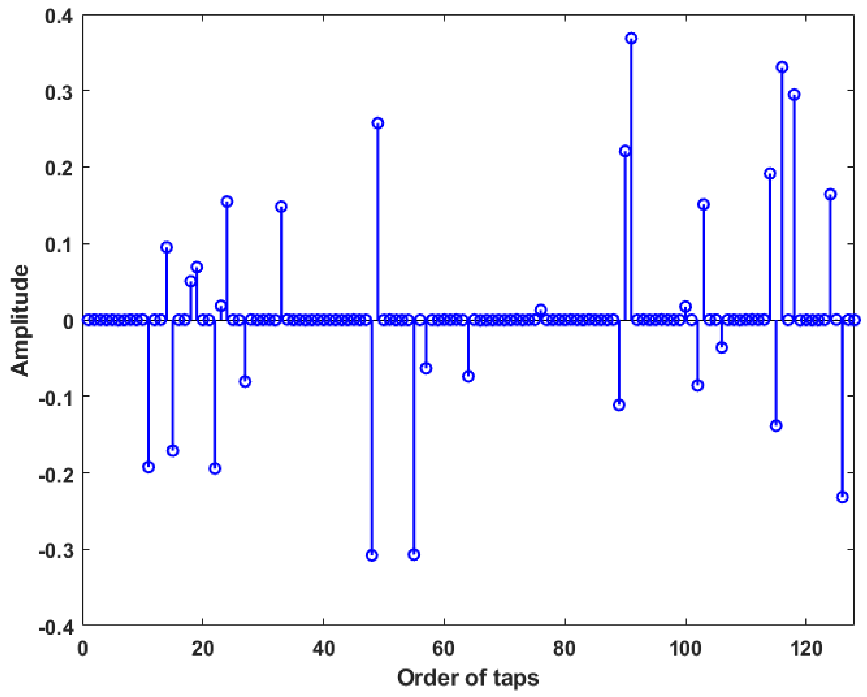
The filter performance of the proposed APSA was evaluated through computer simulations involving system-identification scenarios. An unknown target system was randomly generated with 128 taps (n = 128) and the adaptive filter and unknown target system were considered to have the same number of taps. Moreover, we set 96 near-zero filter coefficients among the 128 taps to establish a general sparse system. The general sparse system has the property of sparsity as shown in Figure 2.

Each adaptive filter was tested for a projection order M = 4. In our simulations, three types of input signal—white input, autoregressive (AR) and autoregressive–moving-average (ARMA)—were used, and correlated input signals for AR and ARMA models were generated by filtering white Gaussian noise through the following systems as

$$\begin{array}{cc}\hfill G_1\left(z\right)& =\frac{1}{1-0.7z^{-1}},\hfill \end{array}$$

(14)

$$\begin{array}{cc}\hfill G_2\left(z\right)& =\frac{1+0.6z^{-1}}{1+z^{-1}+0.21z^{-2}}.\hfill \end{array}$$

(15)

The signal-to-noise ratio (SNR) was set to 30 dB for adding the measurement noise at the output signal $y_i$. The SNR is defined by $y_i={\mathbf{u}}_i^T{\mathbf{w}}_o$ as follows:

$$\mathrm{SNR}\triangleq 10lo{g}_{10}\left(\frac{E\left[y_i^2\right]}{E\left[v_i^2\right]}\right).$$

(16)

The impulsive noise $n_i$ was generated as $n_i=k_i{A}_i$ where $k_i$ represents a Bernoulli process with a probability of success $P[k_i=1]=Pr$, and $A_i$ represents zero-mean Gaussian noise with the power ${\sigma }_A^2=1000{\sigma }_y^2$ [11,13]. $Pr$, which denotes the probability of the occurrence of impulsive noise, was set to 0.001. The normalized mean squared deviation (NMSD) was defined as

$$\mathrm{NMSD}\triangleq 10{log}_{10}\left(\frac{E\left[{\tilde{\mathbf{w}}}^T\left(k\right)\tilde{\mathbf{w}}\left(k\right)\right]}{{\mathbf{w}}_o^T{\mathbf{w}}_o}\right),$$

(17)

where the filter-coefficient error vector ${\tilde{\mathbf{w}}}_i\triangleq {\mathbf{w}}_o-{\widehat{\mathbf{w}}}_i$. The results were obtained via ensemble averaging over 100 trials.

4.1. System Identification for Sparse System in Presence of Impulsive Noises

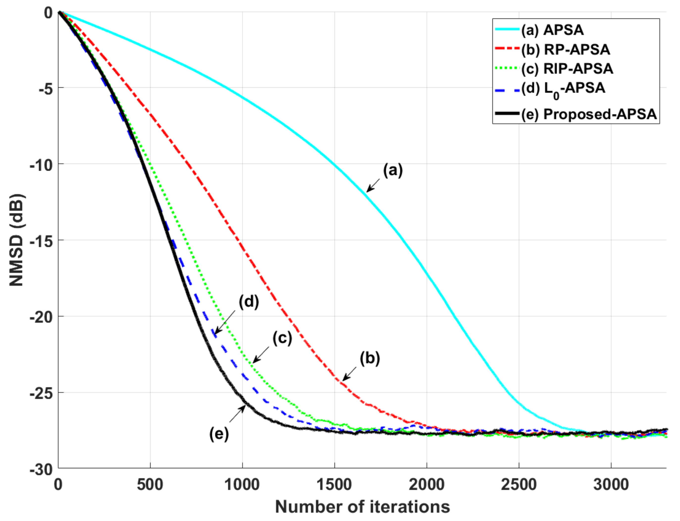
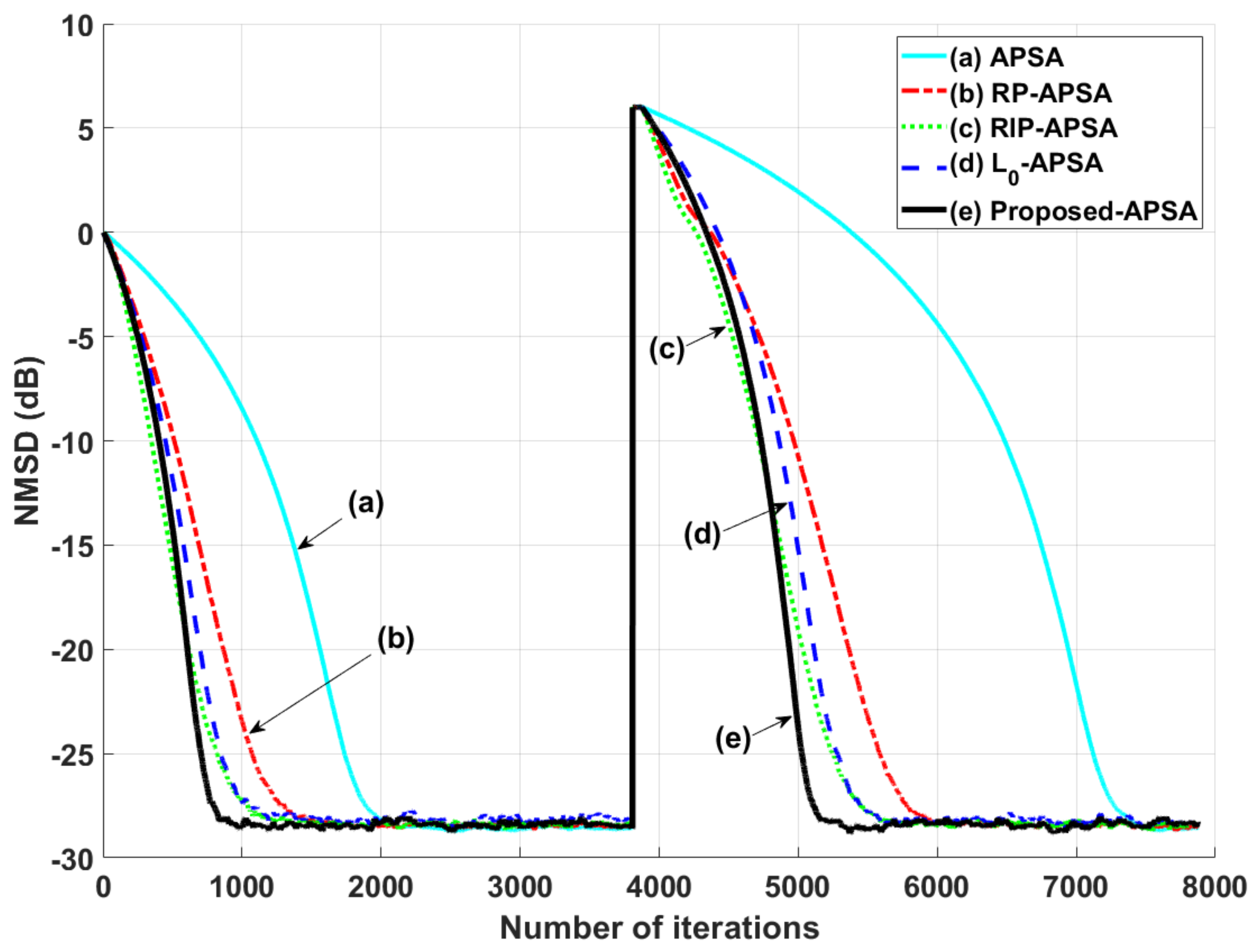
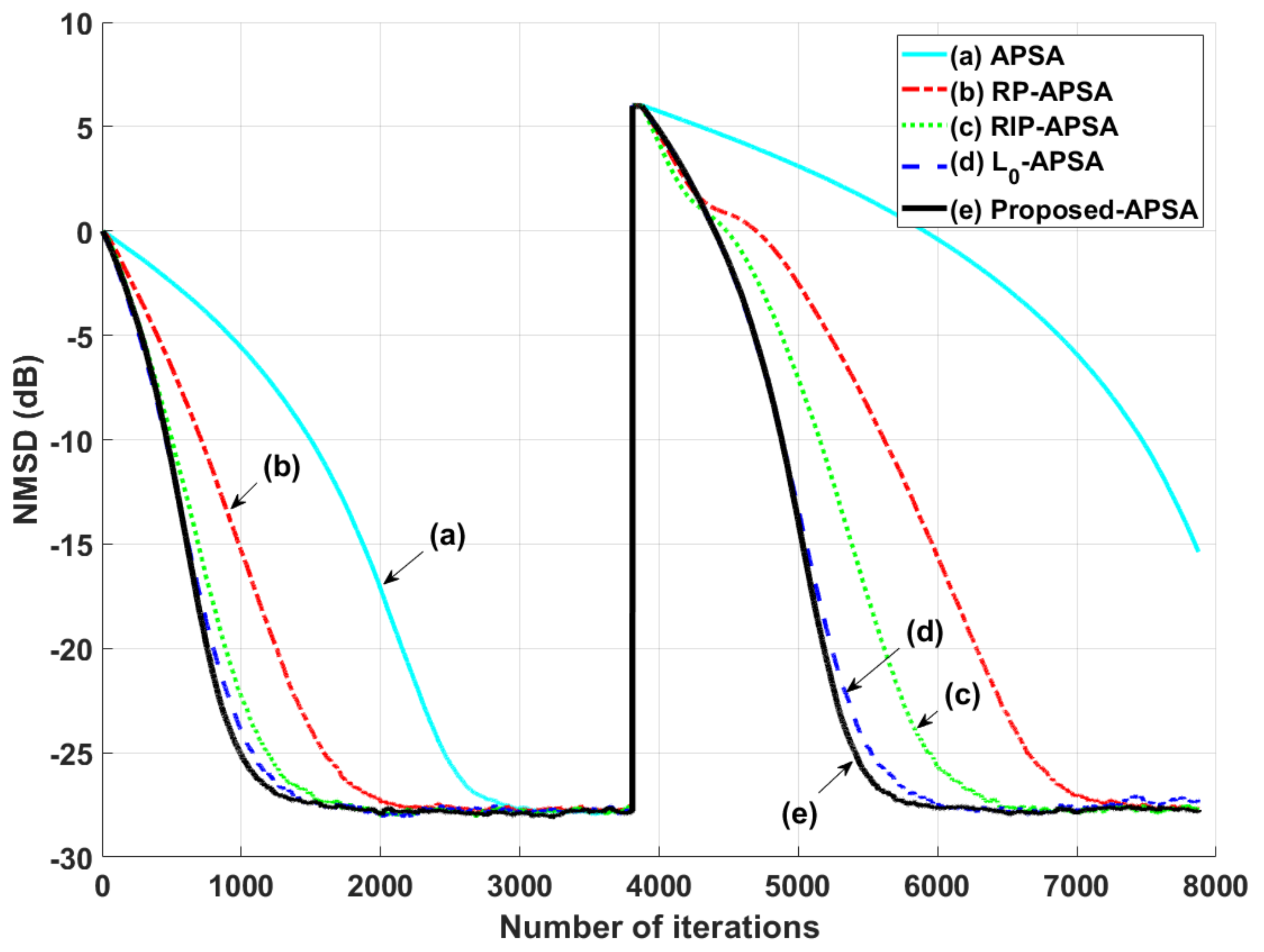
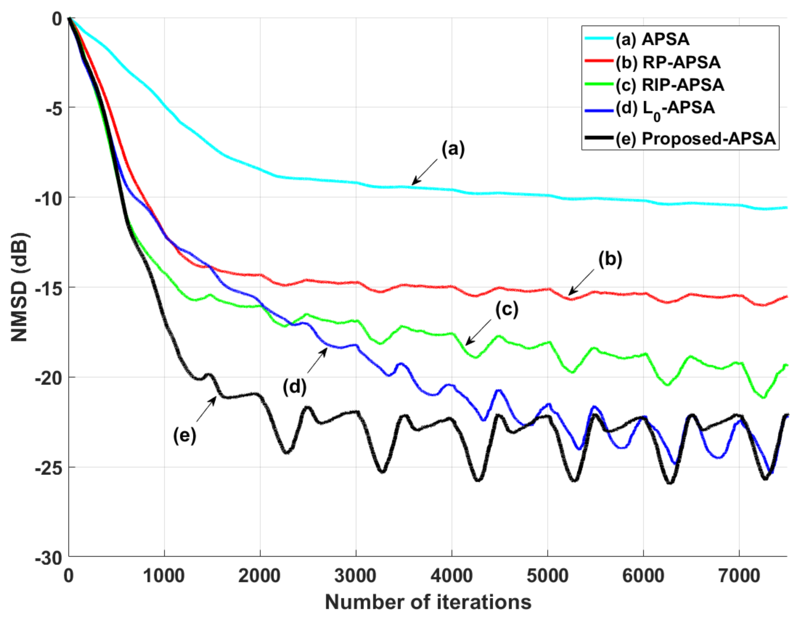
Figure 3 shows the NMSD learning curves for the original APSA [11], RP-APSA [12], RIP-APSA [12], ${\mathcal{L}}_0$-APSA [13] and proposed APSA with white input signals. Figure 4 and Figure 5 also indicate the NMSD learning curves for the original APSA, RP-APSA, RIP-APSA, ${\mathcal{L}}_0$-APSA and the proposed APSA with correlated input signals $G_1\left(z\right)$ and $G_2\left(z\right)$, respectively. According to Figure 3, Figure 4 and Figure 5, the proposed ${\mathcal{L}}_p$-norm-like APSA has a faster convergence rate than the existing algorithms when the representative white, AR and ARMA input signals were used. Because the convergence rate and steady-state estimation errors have a trade-off relationship, we focus on the comparison in aspects of the convergence rate. To ensure a fair comparison of the convergence rate of the proposed APSA and other algorithms, the algorithm parameters were selected such that the steady-state errors for all the algorithms were identical. Specifically, the parameters were set as follows: APSA ($\mu =0.005$); RP-APSA ($\mu =0.007,p=0.1$); RIP-APSA ($\mu =0.009,\alpha =0$); ${\mathcal{L}}_0$-APSA ($\mu =0.022,\beta =20,\gamma =0.003$); and the proposed APSA ($\mu =0.017$ for the white input/$\mu =0.02$ for $G_1\left(z\right),G_2\left(z\right)$ and speech input, $\gamma =0.03$, $p=0.1$, $ϵ=0.01$). To set almost the same convergence rate for all algorithms, the step sizes of the proposed algorithm for the white input are slightly slight difference compared to those of the AR and ARMA cases. The p parameter of RP-APSA and the $\alpha$ parameter of RIP-APSA were set with reference to an existing study [12] for fair comparison. As shown in Figure 1 and Figure 2, the proposed APSA exhibited a higher convergence rate than those of the other algorithms. In addition, the proposed APSA maintains filter performance in terms of the convergence rate even though the system change suddenly occurs—as shown in Figure 6, Figure 7 and Figure 8.

4.2. Speech Input Test Including a Double-Talk Situation

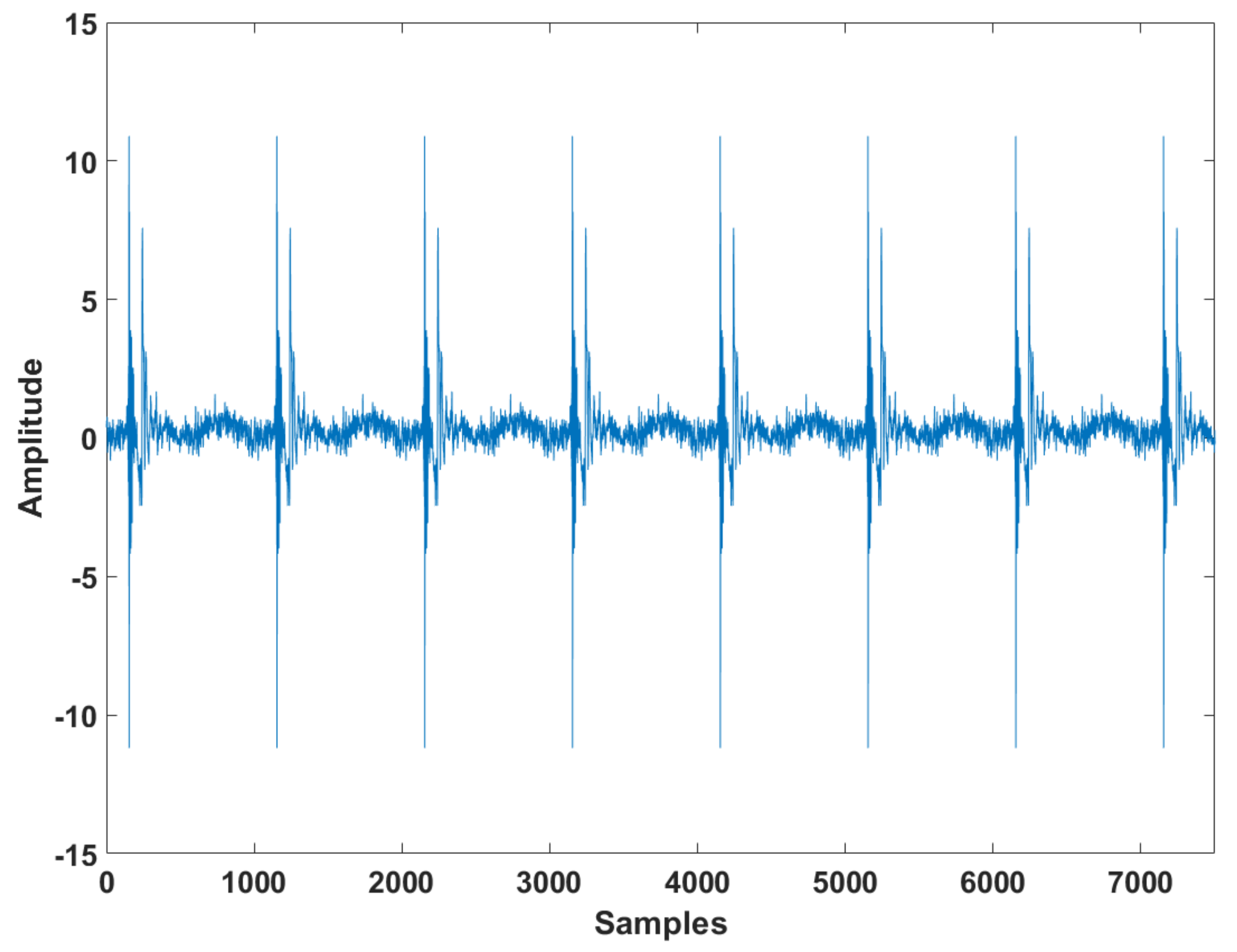
The proposed APSA was subjected to an experiment using a speech input signal to ensure the filter performance in practical scenarios, as can be seen in Figure 9. Since speech input signals are real human speech data, this simulation result for speech input increases the reliability of the proposed APSA for the practical use. As can be seen in Figure 10, we can find that the proposed APSA can accomplish a faster convergence rate and smaller steady-state estimation errors compared to the other algorithms. The proposed algorithm was also tested in a double-talk situation as shown in Figure 11. The far-end input signal and near-end input signal were speech signals where the power of the near-end input signal was two times greater than that of the far-end input signal. The near-end input signal was added between iterations $5.2\times {10}^3$ and $6.2\times {10}^3$. Figure 11 shows that the proposed APSA delivered better performance than the other algorithms in terms of the convergence rate and the steady-state estimation error. Even after the double-talk occurrence, we found that the proposed APSA consistently has smaller steady-state estimation errors.

4.3. Practical Considerations for the p Parameter

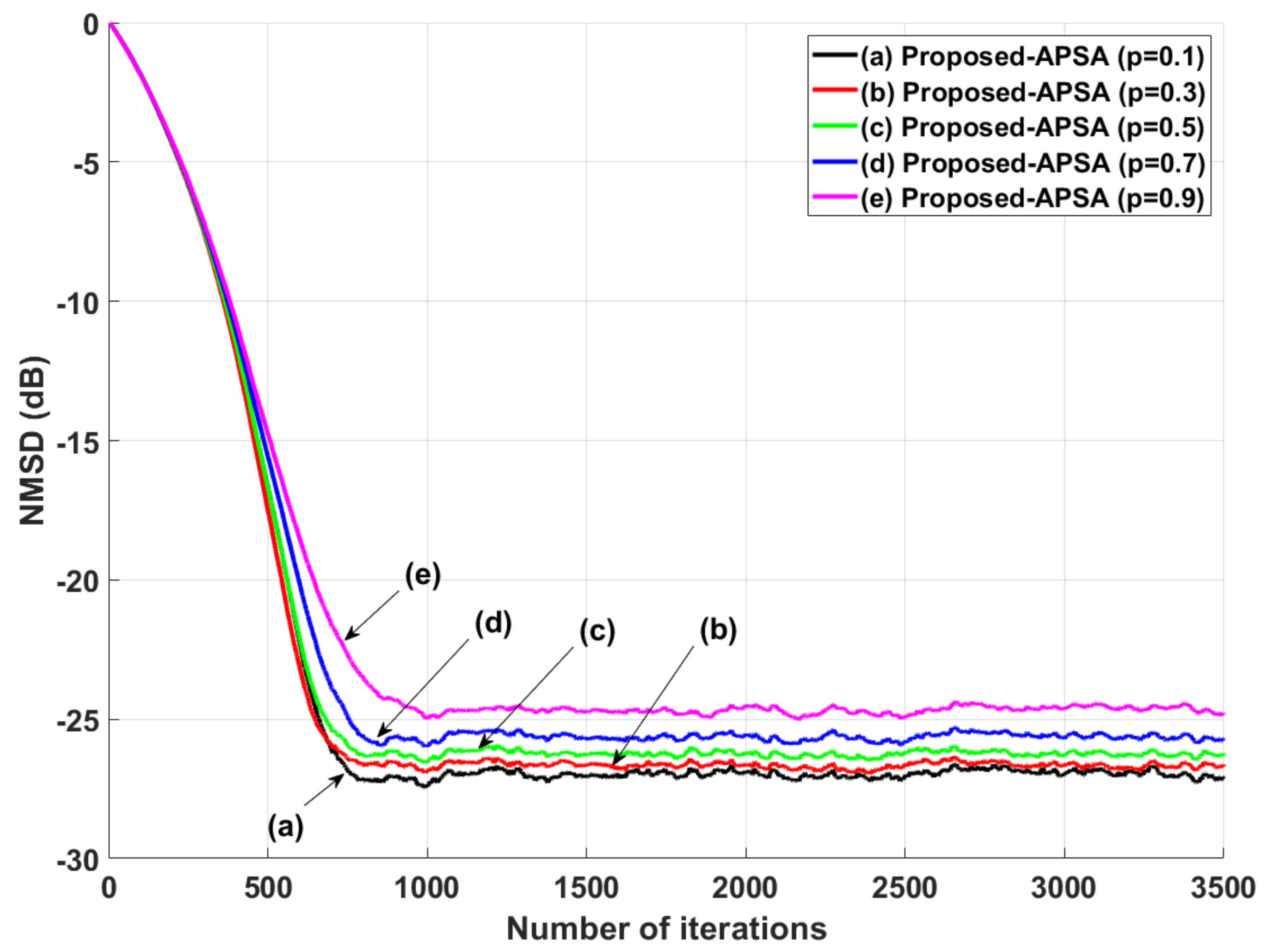
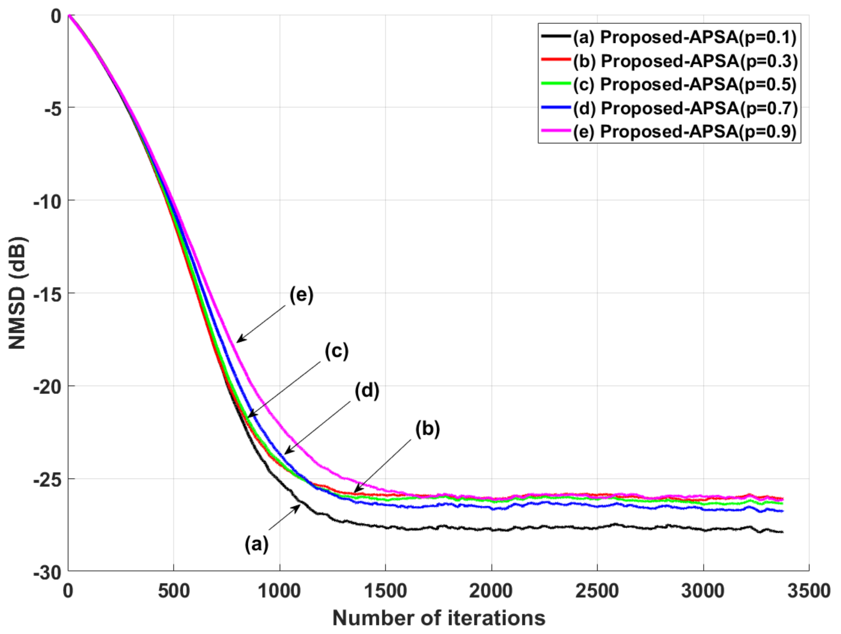
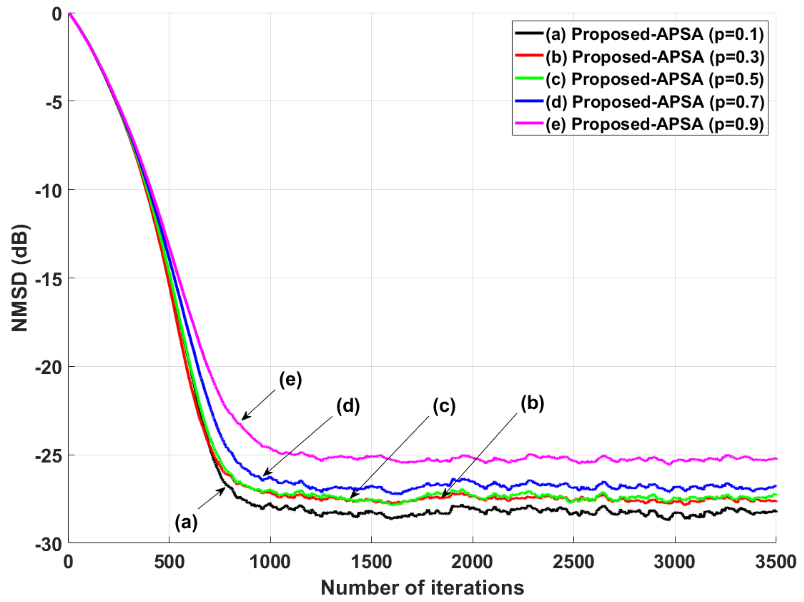
Through Equation (19), we can analyze that when the p parameter is close to 0, the proposed ${\mathcal{L}}_p$-norm-like APSA is the same as the ${\mathcal{L}}_0$-norm APSA. Moreover, the better filter performance of the proposed APSA compared to the ${\mathcal{L}}_0$-norm APSA is demonstrated via Figure 3, Figure 4, Figure 5, Figure 6, Figure 7 and Figure 8 and Figure 10 and Figure 11. On the other hand, if the p parameter is close to 1 as can be seen in Equation (20), the proposed ${\mathcal{L}}_p$-norm-like APSA is similar to the ${\mathcal{L}}_1$-norm APSA that does not have the advantages for the sparse system due to the characteristic of the ${\mathcal{L}}_1$ norm. Therefore, it is meaningful to choose the specific p value between 0 and 1 to improve the filter performance of the proposed APSA and there is no advanced research for the APSA-type algorithms using the proposed ${\mathcal{L}}_p$-norm-like concept. We find that the specific p value can maximize the improvement of our proposed algorithm through the parameter tuning method, as shown in Figure 12, Figure 13 and Figure 14. As shown in Figure 12, Figure 13 and Figure 14, the specific p value consistently verifies the improved filter performance regardless of the white, ar and arma input signals. When the p parameter is set to 0.1, the proposed APSA has the best filter performance, achieving a fast convergence rate and small steady-state estimation errors. Even though the parameter tuning method cannot precisely provide optimal value, $p=0.1$ gives the best performance in our simulation scenarios. Since the parameter p value has a restriction between 0 and 1, it is easy to find the proper p value according to the variation of p values to adequately guarantee the improved filter performance in each scenario.

It is important to decide the p parameter in the proposed APSA because the effect of the p value is dominant in adjusting the filter performance in terms of convergence rate and steady-state estimation errors. The ${\mathcal{L}}_p$-norm-like definition can be represented by

$$\left|\right|{\widehat{\mathbf{w}}}_i{\left|\right|}_p^p=\sum _{k=0}^{n-1}{\left|{\widehat{w}}_i\left(k\right)\right|}^p,0\le p\le 1.$$

(18)

From Equation (18), we can derive the ${\mathcal{L}}_0$-norm term and the ${\mathcal{L}}_1$-norm term by adjusting the p value as follows:

$$\begin{array}{cc}\hfill & \underset{p\to 0}{lim}\left|\right|{\widehat{\mathbf{w}}}_i{\left|\right|}_p^p=\left|\right|{\widehat{\mathbf{w}}}_i{\left|\right|}_0=\#\left\{k\right|{\widehat{w}}_i\left(k\right)\ne 0\},\hfill \end{array}$$

(19)

$$\begin{array}{cc}\hfill & \underset{p\to 1}{lim}\left|\right|{\widehat{\mathbf{w}}}_i{\left|\right|}_p^p=\left|\right|{\widehat{\mathbf{w}}}_i{\left|\right|}_1=\sum _{k=0}^{n-1}\left|{\widehat{w}}_i\left(k\right)\right|.\hfill \end{array}$$

(20)

5. Conclusions

An improved affine projection sign algorithm for sparse system identification was developed using a ${\mathcal{L}}_p$-norm-like constraint. The ${\mathcal{L}}_p$-norm-like constraint could accelerate the convergence of the near-zero coefficients of a general sparse system. Moreover, a novel cost function including the ${\mathcal{L}}_p$-norm-like constraint was used for the proposed APSA. Consequently, the convergence rate of the proposed APSA was higher than those of the original APSA, RP-APSA, RIP-APSA and ${\mathcal{L}}_0$-APSA, as demonstrated by simulation results.

References

1. Zhang, R.; Zhao, H. A Novel Method for Online Extraction of Small-Angle Scattering Pulse Signals from Particles Based on Variable Forgetting Factor RLS Algorithm. Sensors 2021, 21, 5759. [Google Scholar]
2. Qian, G.; Wang, S.; Lu, H.H.C. Maximum Total Complex Correntropy for Adaptive Filter. IEEE Trans. Signal Process. 2020, 68, 978–989. [Google Scholar] [CrossRef]
3. Shen, L.; Zakharov, Y.; Henson, B.; Morozs, N.; Mitchell, P.D. Adaptive filtering for full-duplex UWA systems with time-varying self-interference channel. IEEE Access 2020, 8, 187590–187604. [Google Scholar] [CrossRef]
4. Dogariu, L.-M.; Stanciu, C.L.; Elisei-Iliescu, C.; Paleologu, C.; Benesty, J.; Ciochina, S. Tensor-Based Adaptive Filtering Algorithms. Symmetry 2021, 13, 481. [Google Scholar] [CrossRef]
5. Kumar, K.; Pandey, R.; Karthik, M.L.N.S.; Bhattacharjee, S.S.; George, N.V. Robust and sparsity-aware adaptive filters: A Review. Signal Process. 2021, 189, 108276. [Google Scholar] [CrossRef]
6. Kivinen, J.; Warmuth, M.K.; Hassibi, B. The p-norm generalization of the LMS algorithm for adaptive filtering. IEEE Trans. Signal Proc. 2006, 54, 1782–1793. [Google Scholar] [CrossRef] [Green Version]
7. Ozeki, K.; Umeda, T. An adaptive filtering algorithm using an orthogonal projection to an affine subspace and its properties. Electron. Commun. Jpn. 1984, 67, 19–27. [Google Scholar] [CrossRef]
8. Jiang, Z.; Li, Y.; Huang, X.; Jin, Z. A Sparsity-Aware Variable Kernel Width Proportionate Affine Projection Algorithm for Identifying Sparse Systems. Symmetry 2019, 11, 1218. [Google Scholar] [CrossRef] [Green Version]
9. Li, G.; Wang, G.; Dai, Y.; Sun, Q.; Yang, X.; Zhang, H. Affine projection mixed-norm algorithms for robust filtering. Signal Process. 2021, 187, 108153. [Google Scholar] [CrossRef]
10. Li, G.; Zhang, H.; Zhao, J. Modified Combined-Step-Size Affine Projection Sign Algorithms for Robust Adaptive Filtering in Impulsive Interference Environments. Symmetry 2020, 12, 385. [Google Scholar] [CrossRef] [Green Version]
11. Shao, T.; Zheng, Y.R.; Benesty, J. An affine projection sign algorithm robust against impulsive interference. IEEE Signal Process. Lett. 2010, 17, 327–330. [Google Scholar] [CrossRef]
12. Yang, Z.; Zheng, Y.R.; Grant, S.L. Proportionate affine projection sign algorithm for network echo cancellation. IEEE Trans. Audio Speech Lang. Process. 2011, 19, 2273–2284. [Google Scholar] [CrossRef]
13. Yoo, J.; Shin, J.; Choi, H.; Park, P. Improved affine projection sign algorithm for sparse system identification. Electron. Lett. 2012, 48, 927–929. [Google Scholar] [CrossRef]
14. Jin, J.; Mei, S. l0 Norm constraint LMS Algorithm for spare system identification. IEEE Signal Process. Lett. 2009, 16, 774–777. [Google Scholar]
15. Li, Y.; Cherednichenko, A.; Jiang, Z.; Shi, W.; Wu, J. A Novel Generalized Group-Sparse Mixture Adaptive Filtering Algorithm. Symmetry 2019, 11, 697. [Google Scholar] [CrossRef] [Green Version]
16. Li, Y.; Wang, Y.; Albu, F.; Jiang, J. A General Zero Attraction Proportionate Normalized Maximum Correntropy Criterion Algorithm for Sparse System Identification. Symmetry 2017, 9, 229. [Google Scholar] [CrossRef] [Green Version]
17. Li, Y.; Wang, Y.; Sun, L. A Proportionate Normalized Maximum Correntropy Criterion Algorithm with Correntropy Induced Metric Constraint for Identifying Sparse Systems. Symmetry 2018, 10, 683. [Google Scholar] [CrossRef] [Green Version]
18. Wu, F.; Tong, F. Gradient optimization p-norm-like constraint LMS algorithm for sparse system estimation. Signal Process. 2013, 93, 967–971. [Google Scholar] [CrossRef]
19. Wu, F.; Tong, F. Non-Uniform Norm Constraint LMS Algorithm for Sparse System Identification. IEEE Commun. Lett. 2013, 17, 385–388. [Google Scholar] [CrossRef]
20. Zayyani, H. Continuous mixed p-norm adaptive algorithm for system identification. IEEE Signal Process. Lett. 2014, 21, 1108–1110. [Google Scholar]
Figure 1. Structure of an adaptive filter in the presence of impulsive noise n i .
Symmetry 13 01916 g001
Figure 2. Characteristics of a general sparse system (n = 128).
Symmetry 13 01916 g002
Figure 3. NMSD learning curves for the white input in a sparse system with impulsive noises (Pr = 0.01).
Symmetry 13 01916 g003
Figure 4. NMSD learning curves for the correlated input generated using G 1 ( z ) in a sparse system with impulsive noises (Pr = 0.01).
Symmetry 13 01916 g004
Figure 5. NMSD learning curves for the correlated input generated using G 2 ( z ) in a sparse system with impulsive noises (Pr = 0.01).
Symmetry 13 01916 g005
Figure 6. NMSD learning curves for the white input in a sparse system with impulsive noises (Pr = 0.01). The system suddenly changes ( w o w o ) at iteration 3.8 × 10 3 ).
Symmetry 13 01916 g006
Figure 7. NMSD learning curves for the correlated input generated using G 1 ( z ) in a sparse system with impulsive noises (Pr = 0.01). The system suddenly changes ( w o w o ) at iteration 3.8 × 10 3 .
Symmetry 13 01916 g007
Figure 8. NMSD learning curves for the correlated input generated using G 2 ( z ) in a sparse system with impulsive noises (Pr = 0.01). The system suddenly changes w o w o ) at iteration 3.8 × 10 3 .
Symmetry 13 01916 g008
Figure 9. Speech input signal.
Symmetry 13 01916 g009
Figure 10. NMSD learning curves for the speech input.
Symmetry 13 01916 g010
Figure 11. NMSD learning curves for the double-talk situation.
Symmetry 13 01916 g011
Figure 12. NMSD learning curves with several values of p to decide the p value to ensure the best filter performance for the white input in a sparse system with impulsive noises (Pr = 0.01).
Symmetry 13 01916 g012
Figure 13. NMSD learning curves with several values of p to decide the p value to ensure the best filter performance for the correlated input generated using G 1 ( z ) in a sparse system with impulsive noises (Pr = 0.01).
Symmetry 13 01916 g013
Figure 14. NMSD learning curves with several values of p to decide the p value to ensure the best filter performance for the correlated input generated using G 2 ( z ) in a sparse system with impulsive noises (Pr = 0.01).
Symmetry 13 01916 g014
Publisher’s Note: MDPI stays neutral with regard to jurisdictional claims in published maps and institutional affiliations.