Abstract
A modified version of a common global optimization method named controlled random search is presented here. This method is designed to estimate the global minimum of multidimensional symmetric and asymmetric functional problems. The new method modifies the original algorithm by incorporating a new sampling method, a new termination rule and the periodical application of a local search optimization algorithm to the points sampled. The new version is compared against the original using some benchmark functions from the relevant literature.
1. Introduction
Global optimization [1] is considered a problem of high complexity with many applications. The problem is defined as the location of the global minimum of a multi-dimensional function :
where is formulated as:
In global optimization, many functional problems that need to be solved can have symmetric solutions—the minimum—without this being the rule. The location of the global optimum finds application in many areas such as physics [2,3], chemistry [4,5], medicine [6,7], economics [8], etc. In modern theory there are two different categories of global optimization methods: the stochastic methods and the deterministic methods. The first category contains the vast majority of methods such as simulated annealing methods [9,10,11], genetic algorithms [12,13,14], tabu search methods [15], particle swarm optimization [16,17,18] etc. A common method that also belongs to stochastic methods is the controlled random search (CRS) method [19], which is a procedure that uses a population of trial solutions. This method initially creates a set with randomly selected points and repeatedly replaces the worst point in that set with a randomly generated point. This process can continue until some termination criterion is satisfied. The CRS method has been used intensively in many problems such as geophysics problems [20,21], optimal shape design problems [22], the animal diet problem [23], the heat transfer problem [24] etc.
This CRS method has been thoroughly analyzed by many researchers in the field, such as the work A of Ali and Storey, where two new variants of the CRS method were proposed [25]. These variants have proposed alternative techniques for the selection of the initial sample set and usage of local search methods. Additionally, Pillo et al. [26] suggested a hybrid CRS method where the base algorithm is combined with a Newton-type unconstrained minimization algorithm [27] to enhance the efficiency of the method in various test problems. Another work is of Kaelo and Ali, in which they suggested [28] some modifications to the method, especially in the new point generation step. Additionally, Filho and Albuquerque have suggested [29] the usage of a distribution strategy to accelerate the controlled random search method. Tsoulos and Lagaris [30] suggested the usage of a new line search method based on genetic algorithms to improve the original CRS method. The current work proposed three major modifications in the CRS method: a new point replacement strategy, a stochastic termination rule and a periodical application of some local search method. The first modification is used to better explore the domain range of the function. The second modification is made in order to achieve a better termination of the method without wasting valuable computational time. The third modification is used in order to speed up the method by applying a small amount of steps of a local search method. The new method introduces a new method to create trial points that was not present in the previous work [30] and also replaces the expensive call-to-line search method with a few calls to a local search optimization method.
The rest of this article is organized as follows: in Section 2, the major steps of the CRS method as well as the proposed modifications are presented; in Section 3, the results from the application of the proposed method on a series of benchmark functions are listed; and finally, in Section 4, some conclusions and guidelines for future research are presented.
2. Method Description
The controlled random search has a series of steps that are described in Algorithm 1. The changes proposed by the new method focus on three points:
- The creation of a test point (New_Point step) is performed using a new procedure described in Section 2.1.
- In the Min_Max step, the stochastic termination rule described in Section 2.2 is used. The aim of this rule is to terminate the method when, with some certainty, no lower minimums are to be found.
- Apply a few steps of a local search procedure after New_Point step in the point. This procedure is used to bring the test points closer to the corresponding minimums. This speeds up the process of searching for new minima, although it obviously leads to an increase in function calls
2.1. A New Method for Trial Points
The proposed technique to compute the trial point is shown in Algorithm 2. According to this, the calculation of the test point does not contain a product with high values as in the basic algorithm, so that the test point is not too far from the centroid. This technique avoids vector jumps from the centroid, where it has great gravity in the calculation for starting the local optimization. This method also considers in the calculation the current minimum point and not only a random point as in the original technique. With this modification, knowledge that has already been found in the past is used to create a new point and in such a way that it is close to the area of attraction of a local minimum.
2.2. A New Stopping Rule
It is quite common in the optimization techniques to use a predefined number of maximum iterations as the stopping rule of the method. Even though this termination rule is easy to implement, it could sometimes require an excessive number of functions calls before termination; therefore, a more sophisticated termination rule is needed. The termination rule proposed here is inspired by [31]. At every iteration k, the variance of the quantity is calculated. If the optimization technique did not manage to find a new estimation of the global minimum for some iterations, then probably the global minimum has been discovered and the algorithm should terminate. The termination rule is defined as follows; terminate when:
The term represents the last iteration where a new global minimum was located.
| Algorithm 1: The original controlled random search method. The basic steps of the method |
| Initialization Step: |
|
| Min_Max Step: |
|
| New_Point Step: |
|
| Update Step: |
|
| Local_Search Step: |
|
The amount decreases continuously over time as either the method will find a lower estimate for the global minimum or the global minimum will have already been found. In addition, this quantity is de facto permanently positive and therefore is a good candidate for use in termination criteria. If the global minimum has already been found or the method is no longer able to find a new estimate for it, then this quantity will tend to zero and therefore we can interrupt the execution of the algorithm when this quantity falls below a value. This value may be a fraction of the value of the last time a new estimate for the global minimum was found. If we want to allow the algorithm to continue for several generations, this fraction can be small, e.g., 0.25. If we want it to stop more immediately, a good estimate for the fraction can be 0.75. A good compromise between these prices is the 0.5 price chosen here.
| Algorithm 2: The steps of the new proposed method to create more efficient trial points for the controlled random search method |
|
3. Experiments
3.1. Test Functions
The modified version of the CRS was tested against the traditional CRS on series of benchmark functions from the relevant literature [32,33]. The following functions were used:
- Bf1 function, defined as:with ;
- Bf2 function:where ;
- Branin function: with .
- CM–Cosine Mixture function:with . In our experiments we have used ;
- Camel function:
- Easom function:with
- Exponential function:In the conducted experiments, the values with were used, and the corresponding functions were denoted as EXP2, EXP4, EXP8, EXP16, EXP32, EXP64, EXP100;
- Goldstein & Price:
- Griewank2 function:
- Gkls function: is a function with w local minima, described in [34] with . In the conducted experiments, we have used and , and the functions are denoted by the labels GKLS250 and GKLS350;
- Guilin–Hills function: and being positive integers. In our experiments, we have used with 50 local minima in each function. The produced functions are entitled GUILIN550 and GUILIN1050;
- Hansen function: , ;
- Hartman 3 function:with and and
- Hartman 6 function:with and and
- Rastrigin function:
- Rosenbrock function:In our experiments we used this function with ;
- Shekel 7 function:
- Shekel 5 function:
- Shekel 10 function:
- Sinusoidal function:In our experiments, we used and , and the corresponding functions are denoted by the labels SINU4, SINU8, SINU16, SINU32;
- Test2N function. This function is given by the equationIn the conducted experiments the n has the values 4, 5, 6, 7;
- Test30N function. This function is given bywith . The function has local minima in the specified range and we used in our experiments.
3.2. Results
In the experiments, two different values were measured: the rejection rate in the New_Point step and the average number of function calls required. In the first case we measured the percentage of points rejected during the New_Point step, i.e., points created that are outside the domain range of the function. All the experiments were conducted 30 times and different seeds for the random number generator were used each time. The local search method that was used in the experiments and denoted as localsearch(x) was a BFGS variant due to Powell [35]. The experiments were conducted on a i7-10700T CPU (Intel, Mountain View, CA, USA) at 2.00 GHz equipped with 16 GB of RAM. The operating system used was Debian Linux and the all the code was compiled using ANSI C++ compiler.
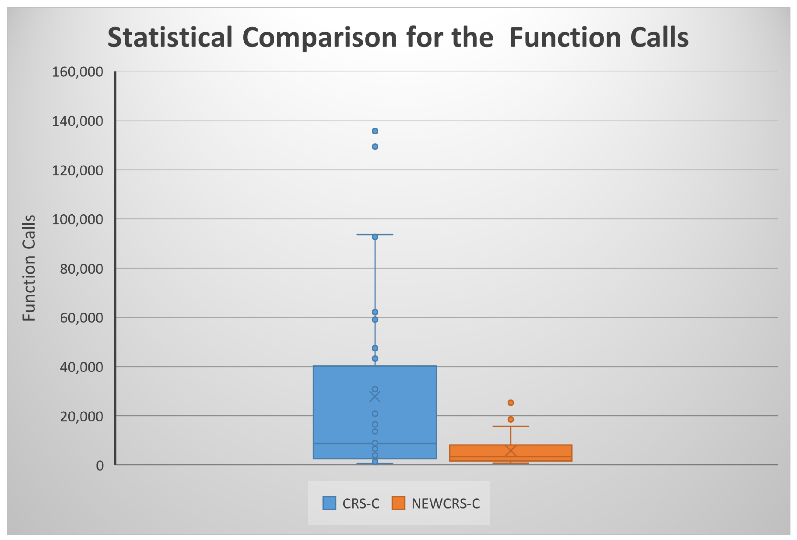
The experimental results are listed in Table 1. The column FUNCTION stands for the name of the objective function. The column CRS-R stands for the rejection rate for the CRS method, while the column NEWCRS-R displays the same measure for the current method. Similarly, the column CRS-C represents the average function calls for the CRS method and the column NEWCRS-C stands for the average function calls of the proposed method. Additionally, a statistical comparison between the CRS and the proposed method is shown in Figure 1.

Table 1.
Experimenting with rejection rates.

Figure 1.
Statistical comparison for the function calls using box plots.
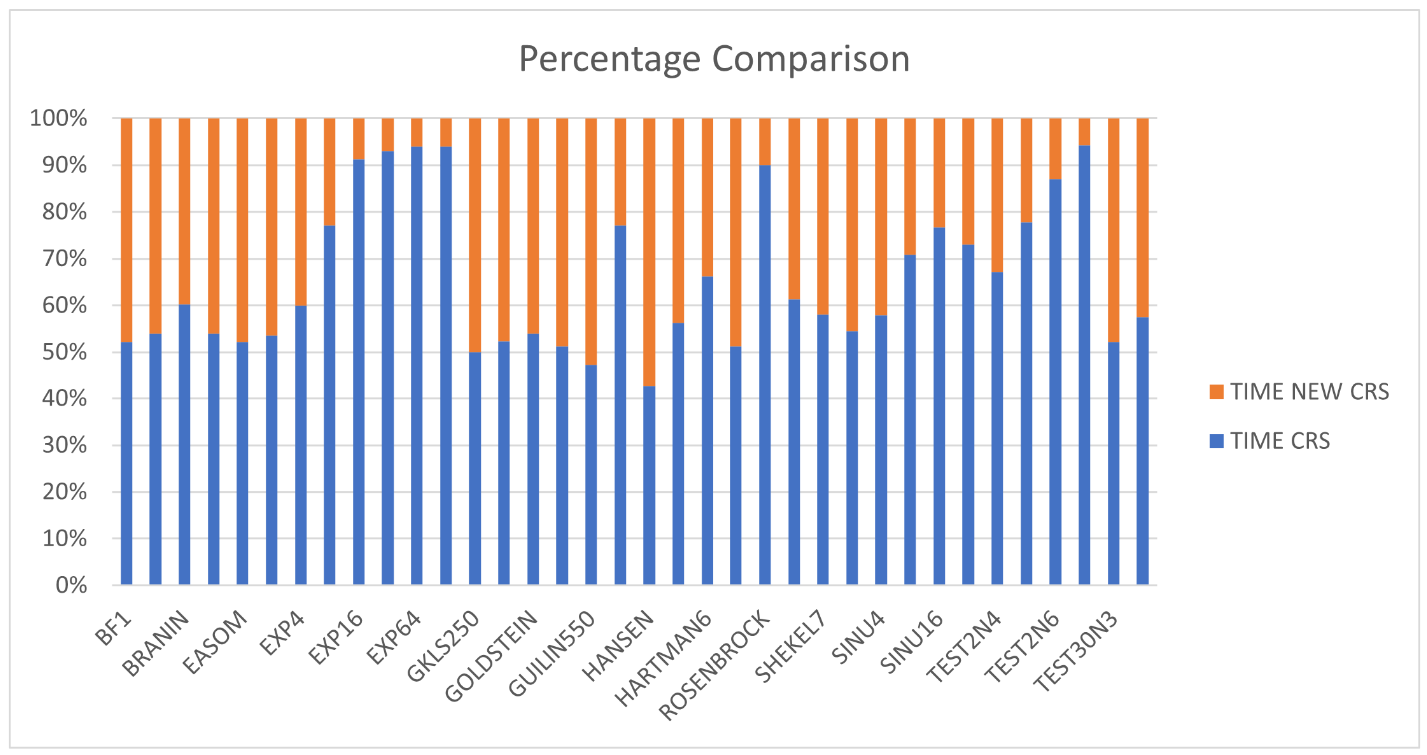
The proposed method almost annihilates the rejection rate in every test function. This is evidence that the new mechanism proposed here to create a new point is more accurate than the traditional one. Additionally, the proposed method requires a lower number of function calls than the CRS method, as one can deduce from the relevant columns and the statistical comparison. The same information is presented graphically in Figure 2, where the percentage comparison of times of functional problems is outlined. Additionally, in the most difficult problems, the proposed method seems to be even more superior to the original one in number of calls, as the combination of the termination rule together with the improved new point generation technique terminate the method much faster and more correctly than the original method.
Figure 2.
Percentage comparison for time execution between the two methods.
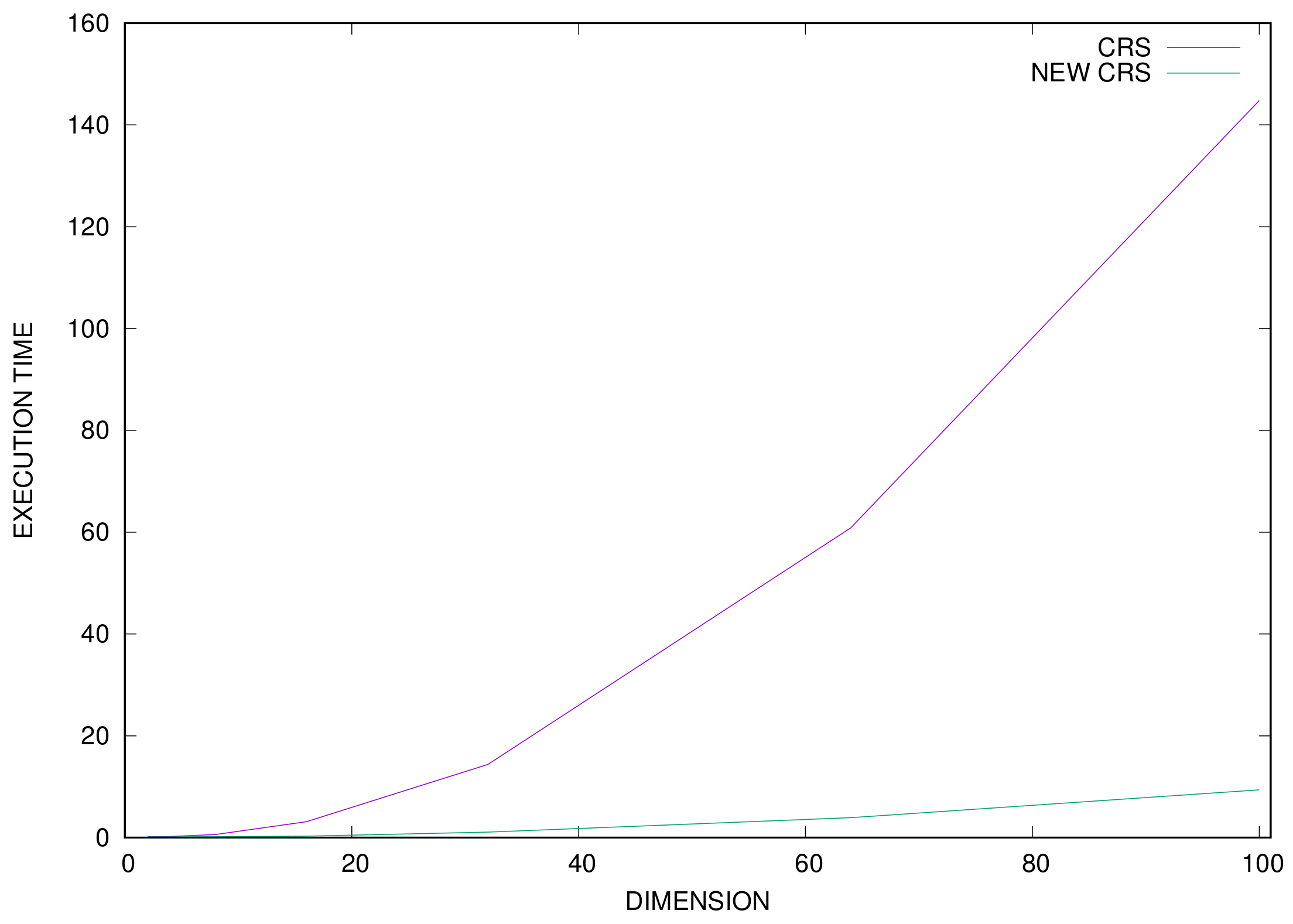
Additionally, the execution time for every test function was measured, and this information is outlined in Table 2. The column CRS-TIME stands for the average execution time of the original CRS method, the column NEWCRS-TIME represents the average execution time for the proposed method and the column DIFF is the calculated percentage difference between the previously mentioned columns. It is evident that the proposed method requires shorter execution times than the original one, and in addition, the difference between the two methods is more obvious in large problems. This phenomenon is also reflected in Figure 3, where a graphical representation of the average execution times of the two methods for the EXP problem for a different number of dimensions is made.

Table 2.
Time comparisons.
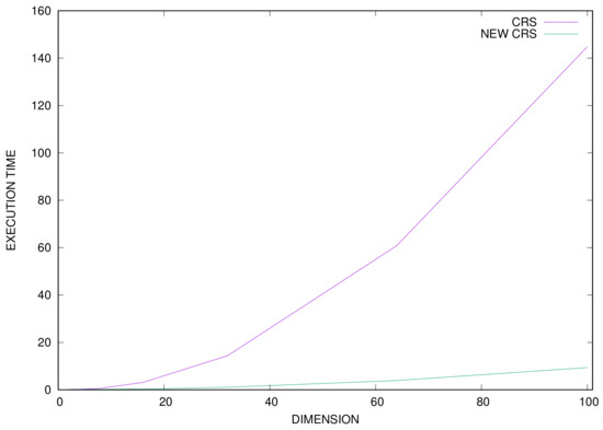
Figure 3.
Time comparison between the two methods for the EXP function for a variety of problem dimensions.
4. Conclusions
Three important modifications were proposed in the current work for the CRS method. The first modification has to do with the new test point generation process, which seems to be more accurate than the original one. The new method creates points that are within the domain range of the function almost every time. The second change adds a new termination rule based on stochastic observations. The third proposed modification applies a few steps of a local search procedure to every trial point created by the algorithm. Judging by the results, it seems that the proposed changes have two important effects. The first is that the success of the algorithm in creating valid test points is significantly improved. The second is the large reduction in the number of function calls required to locate the global minimum.
Future research may include the exploration of the usage of additional stopping rules and the parallelization of different aspects of the method in order to speed up the optimization procedure as well as to take advantage of multicore programming environments.
Author Contributions
V.C., I.T., A.T. and N.A. conceived of the idea and methodology and supervised the technical part regarding the software for the estimation of the global minimum of multidimensional symmetric and asymmetric functional problems. V.C. and I.T. conducted the experiments, employing several different functions, and provided the comparative experiments. A.T. performed the statistical analysis. V.C. and all other authors prepared the manuscript. V.C., N.A. and I.T. organized the research team and A.T. supervised the project. All authors have read and agreed to the published version of the manuscript.
Funding
This research received no external funding.
Institutional Review Board Statement
Not applicable.
Informed Consent Statement
Not applicable.
Data Availability Statement
Not applicable.
Acknowledgments
We acknowledge support of this work from the project “Immersive Virtual, Augmented and Mixed Reality Center of Epirus” (MIS 5047221) which is implemented under the Action “Reinforcement of the Research and Innovation Infrastructure”, funded by the Operational Programme “Competitiveness, Entrepreneurship and Innovation” (NSRF 2014-2020) and co-financed by Greece and the European Union (European Regional Development Fund).
Conflicts of Interest
The authors declare no conflicts.
References
- Törn, A.; Žilinskas, A. Global Optimization Volume 350 of Lecture Notes in Computer Science; Springer: Heidelberg, Germany, 1987. [Google Scholar]
- Yapo, P.O.; Gupta, H.V.; Sorooshian, S. Multi-objective global optimization for hydrologic models. J. Hydrol. 1998, 204, 83–97. [Google Scholar] [CrossRef] [Green Version]
- Duan, Q.; Sorooshian, S.; Gupta, V. Effective and efficient global optimization for conceptual rainfall-runoff models. Water Resour. Res. 1992, 28, 1015–1031. [Google Scholar] [CrossRef]
- Wales, D.J.; Scheraga, H.A. Global Optimization of Clusters, Crystals, and Biomolecules. Science 1999, 27, 1368–1372. [Google Scholar] [CrossRef] [Green Version]
- Pardalos, P.M.; Shalloway, D.; Xue, G. Optimization methods for computing global minima of nonconvex potential energy functions. J. Glob. Optim. 1994, 4, 117–133. [Google Scholar] [CrossRef]
- Balsa-Canto, E.; Banga, J.R.; Egea, J.A.; Fernandez-Villaverde, A.; de Hijas-Liste, G.M. Global Optimization in Systems Biology: Stochastic Methods and Their Applications. In Advances in Systems Biology. Advances in Experimental Medicine and Biology; Goryanin, I., Goryachev, A., Eds.; Springer: New York, NY, USA, 2012; Volume 736. [Google Scholar] [CrossRef] [Green Version]
- Boutros, P.C.; Ewing, A.D.; Ellrott, K.; Norman, T.C.; Dang, K.K.; Hu, Y.; Kellen, M.R.; Suver, C.; Bare, J.C.; Stein, L.D.; et al. Global optimization of somatic variant identification in cancer genomes with a global community challenge. Nat. Genet. 2014, 46, 318–319. [Google Scholar] [CrossRef] [PubMed] [Green Version]
- Gaing, Z.-L. Particle swarm optimization to solving the economic dispatch considering the generator constraints. IEEE Trans. Power Syst. 2003, 18, 1187–1195. [Google Scholar] [CrossRef]
- Kirkpatrick, S.; Gelatt, C.D.; Vecchi, M.P. Optimization by simulated annealing. Science 1983, 220, 671–680. [Google Scholar] [CrossRef]
- Ingber, L. Very fast simulated re-annealing. Math. Comput. Model. 1989, 12, 967–973. [Google Scholar] [CrossRef] [Green Version]
- Eglese, R.W. Simulated annealing: A tool for operational research. Simulated Anneal. Tool Oper. Res. 1990, 46, 271–281. [Google Scholar] [CrossRef]
- Goldberg, D. Genetic Algorithms in Search, Optimization and Machine Learning; Addison-Wesley Publishing Company: Reading, MA, USA, 1989. [Google Scholar]
- Michaelewicz, Z. Genetic Algorithms + Data Structures = Evolution Programs; Springer: Berlin, Germany, 1996. [Google Scholar]
- Grady, S.A.; Hussaini, M.Y.; Abdullah, M.M. Placement of wind turbines using genetic algorithms. Renew. Energy 2005, 30, 259–270. [Google Scholar] [CrossRef]
- Duarte, A.; Martí, R.; Glover, F.; Gortazar, F. Hybrid scatter tabu search for unconstrained global optimization. Ann. Oper. Res. 2011, 183, 95–123. [Google Scholar] [CrossRef]
- Kennedy, J.; Eberhart, R. Particle swarm optimization. In Proceedings of the ICNN’95—International Conference on Neural Networks, Perth, WA, Australia, 27 November–1 December 1995; Volume 4, pp. 1942–1948. [Google Scholar] [CrossRef]
- Poli, R.; Kennedy, J.K.; Blackwell, T. Particle swarm optimization An Overview. Swarm Intell. 2007, 1, 33–57. [Google Scholar] [CrossRef]
- Trelea, I.C. The particle swarm optimization algorithm: Convergence analysis and parameter selection. Inf. Process. Lett. 2003, 85, 317–325. [Google Scholar] [CrossRef]
- Price, W.L. Global Optimization by Controlled Random Search. Comput. J. 1977, 20, 367–370. [Google Scholar] [CrossRef] [Green Version]
- Smith, D.N.; Ferguson, J.F. Constrained inversion of seismic refraction data using the controlled random search. Geophysics 2000, 65, 1622–1630. [Google Scholar] [CrossRef]
- Bortolozo, C.A.; Porsani, J.L.; dos Santos, F.A.M.; Almeida, E.R. VES/TEM 1D joint inversion by using Controlled Random Search (CRS) algorithm. J. Appl. Geophys. 2015, 112, 157–174. [Google Scholar] [CrossRef]
- Haslinger, J.; Jedelský, D.; Kozubek, T.; Tvrdík, J. Genetic and Random Search Methods in Optimal Shape Design Problems. J. Glob. Optim. 2000, 16, 109–131. [Google Scholar] [CrossRef]
- Gupta, R.; Chandan, M. Use of “Controlled Random Search Technique for Global Optimization” in Animal Diet Problem. Int. J. Emerg. Technol. Adv. Eng. 2013, 3, 284–287. [Google Scholar]
- Mehta, R.C.; Tiwari, S.B. Controlled random search technique for estimation of convective heat transfer coefficient. Heat. Mass. Transfer. 2007, 43, 1171–1177. [Google Scholar] [CrossRef]
- Ali, M.M.; Storey, C. Modified Controlled Random Search Algorithms. Int. J. Comput. Math. 1994, 53, 229–235. [Google Scholar] [CrossRef]
- Di Pillo, G.; Lucidi, S.; Palagi, L.; Roma, M. A Controlled Random Search Algorithm with Local Newton-type Search for Global Optimization. In High Performance Algorithms and Software in Nonlinear Optimization. Applied Optimization; De Leone, R., Murli, A., Pardalos, P.M., Toraldo, G., Eds.; Springer: Boston, MA, USA, 1998; Volume 24. [Google Scholar] [CrossRef] [Green Version]
- Lucidi, S.; Rochetich, F.; Roma, M. Curvilinear stabilization techniques for truncated Newton methods in large scale unconstrained optimization. Siam J. Optim. 1998, 8, 916–939. [Google Scholar] [CrossRef]
- Kaelo, P.; Ali, M.M. Some Variants of the Controlled Random Search Algorithm for Global Optimization. J. Optim. Appl. 2006, 130, 253–264. [Google Scholar] [CrossRef]
- Manzanares-filho, N.; Albuquerque, R.B.F. Accelerating Controlled Random Search Algorithms Using a Distribution Strategy. In Proceedings of the EngOpt 2008—International Conference on Engineering Optimization, Rio de Janeiro, Brazil, 1–5 June 2008. [Google Scholar]
- Tsoulos, I.G.; Lagaris, I.E. Genetically controlled random search: A global optimization method for continuous multidimensional functions. Comput. Phys. Commun. 2006, 174, 152–159. [Google Scholar] [CrossRef]
- Tsoulos, I.G. Modifications of real code genetic algorithm for global optimization. Appl. Math. Comput. 2008, 203, 598–607. [Google Scholar] [CrossRef]
- Ali, M.M.; Khompatraporn, C.; Zabinsky, Z.B. A Numerical Evaluation of Several Stochastic Algorithms on Selected Continuous Global Optimization Test Problems. J. Glob. Optim. 2005, 31, 635–672. [Google Scholar] [CrossRef]
- Floudas, C.A.; Pardalos, P.M.; Adjiman, C.; Esposoto, W.; Gümüs, Z.; Harding, S.; Klepeis, J.; Meyer, C.; Schweiger, C. Handbook of Test Problems in Local and Global Optimization; Kluwer Academic Publishers: Dordrecht, The Netheralnds, 1999. [Google Scholar]
- Gaviano, M.; Ksasov, D.E.; Lera, D.; Sergeyev, Y.D. Software for generation of classes of test functions with known local and global minima for global optimization. ACM Trans. Math. Softw. 2003, 29, 469–480. [Google Scholar] [CrossRef]
- Powell, M.J.D. A Tolerant Algorithm for Linearly Constrained Optimization Calculations. Math. Program. 1989, 45, 547–566. [Google Scholar] [CrossRef]
Publisher’s Note: MDPI stays neutral with regard to jurisdictional claims in published maps and institutional affiliations. |
© 2021 by the authors. Licensee MDPI, Basel, Switzerland. This article is an open access article distributed under the terms and conditions of the Creative Commons Attribution (CC BY) license (https://creativecommons.org/licenses/by/4.0/).

