Abstract
Density clustering has been widely used in many research disciplines to determine the structure of real-world datasets. Existing density clustering algorithms only work well on complete datasets. In real-world datasets, however, there may be missing feature values due to technical limitations. Many imputation methods used for density clustering cause the aggregation phenomenon. To solve this problem, a two-stage novel density peak clustering approach with missing features is proposed: First, the density peak clustering algorithm is used for the data with complete features, while the labeled core points that can represent the whole data distribution are used to train the classifier. Second, we calculate a symmetrical FWPD distance matrix for incomplete data points, then the incomplete data are imputed by the symmetrical FWPD distance matrix and classified by the classifier. The experimental results show that the proposed approach performs well on both synthetic datasets and real datasets.
1. Introduction
Clustering analysis is a main technique used to solve the problems that exist in data mining. It aims to classify data points into several groups called clusters so that similar elements are clustered into one group, while different elements are separated from each other [1]. Because clustering can be used to deeply mine internal and possible knowledge, rules, and patterns, it has been applied to many practical fields, including data mining, pattern recognition, machine learning, information retrieval, and image analysis [2,3,4]. Clustering has been widely and intensely studied by the data mining community in recent years. Many clustering algorithms have been proposed: K-means [5], fuzzy C-means [6], affinity propagation [7], Gaussian mixtures [8], etc. These algorithms perform well on many occasions, but they cannot deal with datasets with arbitrary shapes, and the determination of hyperparameters and clustering centers is also difficult for clustering algorithms.
Density-based clustering methods (such as DBSCAN) [9,10] consider clusters as high-density regions separated by low-density regions. DBSCAN can process datasets with arbitrary shapes. However, it is sensitive to the density radius parameter, and small parameter changes can lead to widely different clustering results. In 2014, Alex and Rodriguez proposed the density peak clustering (DPC) algorithm [11] in Science, a novel fast density peak clustering algorithm that can recognize clusters with arbitrary shapes without setting the number of clusters in advance. Compared to a traditional clustering algorithm, DPC can quickly identify cluster centers, needs few parameters, has a fast clustering speed, and can be used with datasets with different shapes. Therefore, several research studies [12,13,14,15,16,17,18] have been performed focusing on this method.
Although the DPC algorithm and its improved version have achieved great success and proved their high performance in practical applications, they can only be used to process complete data. However, in many practical applications, we may encounter missing features for various reasons (such as sensor failure, measurement error, unreliable features, etc.).
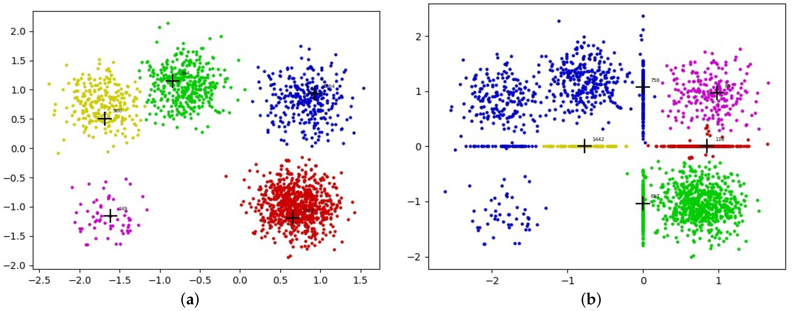
Researchers have expended considerable effort to study the problem of incomplete data. Some methods have been proposed for supervised learning and unsupervised learning [19,20,21,22,23]. A simple way is to discard those missing values by eliminating instances that contain missing values before clustering. More commonly, the missing data are imputed by an imputation algorithm (such as zero imputation, mean imputation, KNN imputation, or EM imputation [24,25,26]) and then clustered by the original clustering algorithm. However, the clustering performance on incomplete data is much lower. Recently, imputation and clustering were considered in the same framework [23,27] to improve the clustering performance on incomplete data, but most of these methods cannot handle incomplete data with arbitrary shapes well. In addition, the imputation-based method does not work well in the DPC algorithm because of the aggregation phenomenon of imputed points. The cluster centers in DPC have a higher density than their neighbors, and the different cluster centers are far away from each other. The example in Figure 1 illustrates the aggregation phenomenon. The five-cluster dataset is a two-dimensional synthetic dataset that contains five clusters. We can accurately obtain five clusters and their centers (the cross mark in Figure 1a) by executing the DPC algorithm on the five-cluster dataset; the results are shown in Figure 1a. For comparison, we can generate missing data by randomly deleting 25% of all features in the five-cluster dataset. Then, the missing feature data points are imputed by the mean imputation method and the DPC algorithm is executed on the missing feature data. The clustering results are shown in Figure 1b. As shown in Figure 1b, the two straight lines in the middle area are the missing feature points imputed by mean imputation, and these imputed data points form some high-density areas, which breaks the assumption of the DPC algorithm. Thus, applying DPC on incomplete data can lead to the wrong centers being chosen (the cross marks in Figure 1b) and to a very poor clustering result. Other advanced imputation algorithms (such as KNN imputation) are also likely to break the assumption of the DPC algorithm and lead to the aggregation phenomenon of imputed data points.
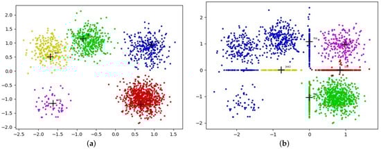
Figure 1.
Aggregation phenomenon. (a) DPC original results on the five-cluster dataset. (b) DPC results on the five-cluster dataset with 25% missing ratio.
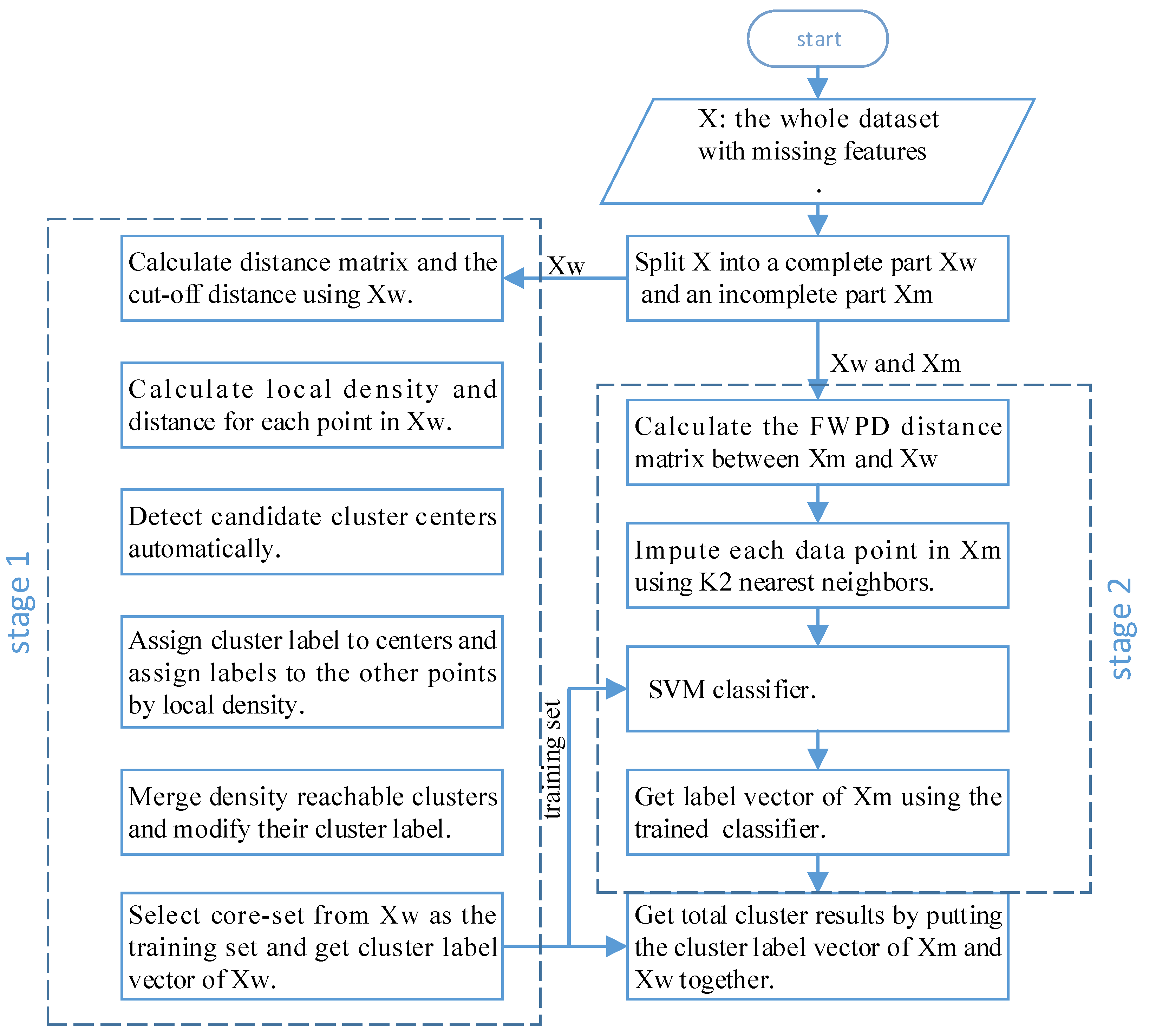
Classification algorithms are highly accurate and can accurately learn the distribution of data, but they need labeled training data. Clustering algorithms do not need data with labels, but the accuracy of the learned model will not be particularly high. In addition, during the label assignment process of DPC, a point is always assigned the same label as the nearest neighbor with a higher density, and errors propagated in the subsequent assignment process. Incomplete points with many missing features are more likely to be assigned a wrong label and propagate errors. Therefore, to avoid the above problems and improve the clustering performance when features of data points are missing, in this paper, we propose the use of a novel two-stage clustering algorithm based on DPC. In stage 1, based on the idea of training a classification model using clustering results, a batch of labeled data is first obtained by density peak clustering, then some representative points are selected. In stage 2, a powerful classifier is trained using these representative points. Then, a symmetrical FWPD distance matrix for incomplete data points is computed, after that, the missing feature data are imputed by the FWPD distance matrix and classified by the classifier. Our algorithm works well with incomplete data while maintaining the advantages of the DPC algorithm. The main diagram of the proposed method is shown in Figure 2. We conducted extensive experiments on three synthetic datasets and six UCI benchmark datasets; the experimental results showed the effectiveness of our proposed algorithm.
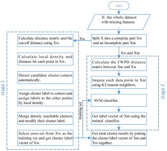
Figure 2.
The main diagram of the DPC-INCOM.
The main contributions of this article are summarized as follows:
(1) To the best of our knowledge, this is the first work about clustering on incomplete data of arbitrary shapes. To solve this problem, we propose combining clustering with classification. The classifier has a high accuracy but it needs labeled data. In stage 1, we use the density clustering method to obtain labeled data, then select some high-quality labeled data to train the classifier in stage 2. Stage 2 relies on the samples from stage 1. Although the original DPC can deal with irregular data, we introduced some improvements, such as improving the local density formula, making it automatically select centers, and merging clusters. Therefore, the clustering performance in stage 1 has obvious advantages. The classifier in stage 2 retains advantages and improves the clustering performance.
(2) Based on the above ideas, we propose a density peak clustering method for incomplete data named DPC-INCOM. The traditional DPC method fails when handling incomplete data due to the aggregation phenomenon. DPC-INCOM can deal with this kind of situation well.
(3) We conducted extensive experiments on three synthetic datasets and six UCI benchmark datasets. Our algorithm achieves superior performance compared to other imputation-based methods.
2. Related Work
2.1. Density Peak Clustering Model and Its Improvements
The DPC algorithm is a powerful clustering method. DPC has two basic assumptions: the first is that cluster centers are surrounded by neighbors with a lower local density; the second is that centers are at a relatively large distance from any points with a higher local density. This method utilizes two major quantities: local density and the distance from points with a higher density , corresponding to the DPC assumption. We now introduce how to calculate them in detail.
Assume that is the whole dataset with N samples, where is the ith vector with M features. The dataset’s distance matrix should be computed first. The local density of data point , denoted by , is defined as:
where is the Euclidean distance between points and , and is the cutoff distance. The procedure for determining is similar to that used to determine the average number of neighbors of all points in a dataset. As a general rule, should be chosen, such that the average number of the neighbors is between 1% and 2% of the total number of points in the dataset. is the number of nodes adjacent to point . The computation of is simple. It is measured by calculating the minimum distance between and any other object of higher density, and is defined as:
Only the data points with a large local density and large distances can become centers (also known as density peaks). The remaining data points will be assigned the same label as their nearest neighbors with a higher local density after the centers are selected. As such, all data points can be assigned a label.
The original DPC algorithm is not sensitive to the local geometric features of the data. Especially when the density difference between clusters is large, the local density difference between cluster centers is also large. Therefore, the local density of centers from low-density clusters is too low. DPC cannot identify the centers from low-density clusters. In addition, the initial cluster centers must be manually rather than automatically selected. However, it is difficult to obtain the correct selection in some datasets. Several research studies [12,13,14,15,16,17,18] have been performed wih this method to overcome these defects. A previous study [13] proposed a new local density calculation method based on K nearest neighbors, effectively identifying the low-density centers without manually setting the parameters .
2.2. Incomplete Data Processing Methods
2.2.1. Some Classical Imputation Methods
The simplest and most commonly used imputation methods are zero imputation, mean imputation, median imputation, and mode imputation. Another common imputation method is K nearest neighbor imputation (KNN) [25], where the missing features of a data point are imputed by the mean value of corresponding features over its K nearest neighbors on the observed subspace. Unlike the approaches described above, Bayesian frameworks use the expectation-maximization (EM) algorithm to deal with incomplete features that imputes missing data values with the most likely estimated values.
2.2.2. Dynamic Imputation Methods
Ref. [28] proposes a dynamic K-means imputation (DK) method. Given a dataset and the number of clusters k, if a sample is an incomplete sample, the DK divides it into two parts: the visible part and the missing part . In the iterative process, DK modifies the imputation value of simultaneously while remains unchanged. DK modifies three variables in each iteration: the data matrix , the allocation matrix H, and the cluster center . Ref. [27] presents another dynamic imputation method based on the Gaussian mixture model. The authors of [23] proposed a novel framework that can cluster mixed numerical and categorical data with missing values. The framework integrates the imputation and clustering steps into a single process and obtained fairly accurate results. These methods work well on many occasions but cannot handle datasets of arbitrary shapes with missing features.
2.2.3. Similarity Measurement of Incomplete Data
Other scholars think that it is not necessary to impute missing features before clustering. Many clustering algorithms judge whether a sample belongs to a cluster based on the similarity measurement of the sample (such as Euclidean distance). Therefore, some scholars directly calculated the similarity or distance between incomplete data points. Hathaway proposed the concept of partial distance (PDS) [29] in 2001. Ref. [30] proposes a different distance measure (FWPD distance) for incomplete data that considers the distribution of missing data. A penalty term is added. It is considered that if most samples do not lose their features but one sample loses them, that one should be given a greater penalty. On the other hand, if there are a large number of missing values in a column, a smaller penalty will be imposed. The author applied FWPD distance in the K-means method and then directly clustered incomplete data points; this achieved excellent results. However, its penalty weight parameters depend on experience and need to be further improved.
2.3. Classification Methods
Classification aims to find a set of models or functions that can describe a dataset’s characteristics and identify the categories of unknown data samples. The classification algorithm mainly includes two steps. The first step involves establishing a model to describe the categories and the distribution of known datasets. The dataset used to train the classifier is named the training set. The second step is to use the obtained model for classification. The most commonly used classification algorithms include the Bayesian method, neural network, and support vector machine (SVM) [31,32,33].
3. Density Peak Clustering with Incomplete Data
3.1. The Problem of Incomplete Data Clustering
The problem of clustering with incomplete data has been the subject of several prior studies [10,29]. Table 1 provides the list of notations used in this paper. Given a set of objects represented by a numerical data matrix , is the kth data vector that describes the object by specifying values for M particular features. The jth component of the data vector is denoted by . In practice, some features of certain data points may be missing in some cases. Such data can be called incomplete data. For example, is incomplete datum, where and are missing. Otherwise, the point is called complete datum. Any dataset containing such points (missing values) can be regarded as an incomplete dataset. For convenience of expression, we use to note that data that no features are missing in the dataset and to note the incomplete part of .

Table 1.
Table of notations.
Problem Statement. Given a dataset with N unlabeled points, each point has M dimensions (features). Based on the features, the clustering algorithm aims to find a set of clusters , where each can mapped to one cluster and . The points in the same cluster should have similar features, while the points far away should never appear in the same cluster. Accordingly, we denote as the cluster label of sample . After, a cluster label vector can be used to represent the clustering result with N elements.
When using the DPC algorithm to process incomplete data, it makes sense to impute the missing features first and then apply the DPC algorithm for imputed data. However, the use of a simple imputation-based method (zero imputation, mean imputation, or median imputation) may lead to the aggregation phenomenon, where some imputed missing feature data points gather and form a high-density area. Thus, their density exceeds that of the original clustering centers, leading to a poor clustering result. Complex imputation methods such as KNN imputation can also suffer from the aggregation phenomenon.
To extend the DPC algorithm to incomplete data, we designed the DPC-INCOM method, which can work well on incomplete data and automatically identify cluster centers without manually setting the number of clusters k. The proposed method divides the clustering problem into two major stages: Stage 1 uses improved DPC to obtain a batch of labeled data samples. The details of this process can be found in Section 3.2 and Section 3.3. In stage 2, the labeled data points with a high local density are selected as a core set, a proper classification model is selected, and the labeled training dataset is fed to train the model. Then, missing feature data samples are imputed with K nearest neighbors. Finally, the trained classifier is used to classify the imputed missing feature data. Section 3.4 provides a detailed description of Stage 2.
3.2. Improved Density Formula
Ref. [13] proposes an improved DPC, which overcomes the shortcoming of DPC: the original algorithm cannot effectively identify the center of low-density clusters. The improved local density is calculated by K nearest neighbors. Therefore, not much difference exists between the local density of the center of a low-density cluster and the local density of the center of a high-density cluster, and this improved algorithm no longer needs to set the parameter . The improved local density of the ith data point is defined as:
where is the number of data points in and is the distance between data point i and its Kth nearest neighbor, being defined as . is the K nearest neighbors of data point i. is the Euclidean distance between data points i and j. Our method borrows this improved density formula to improve the performance of Stage 1. Note that any improvement in DPC can be applied in Stage 1.
3.3. Automatic Selection of Centers and Cluster Merging
A decision graph must be established in the original DPC algorithm and then the cluster centers must be manually selected. If the cutoff distance parameter is incorrect, the decision graph may be incorrectly built. In addition, the original algorithm assumes that there is only one density peak in one cluster. If there are multiple density peaks, DPC cannot cluster correctly. The subsequent assignment procedure will propagate errors, but no action is taken in the DPC to fix them. It should also be pointed out that the initial cluster centers are selected manually rather than automatically. However, it is difficult to obtain the correct selection in some datasets. For the same decision graph, different people choose different cluster centers, and the clustering results will therefore different. To solve these problems, we propose a method that involves automatically selecting cluster centers and automatically merging density reachable clusters.
3.3.1. Candidate Centers
According to the local density and distance , we set a threshold and then select the candidate centers according to this threshold. Candidate centers are defined as:
where and are the local density and distance of the ith data point , respectively, and is the representative data point. is the product of the local density and distance of , and should be larger than the other of the data points. is a constant number and can usually be set as 1. Using this threshold, we can select points with a relatively high local density and distance as candidate cluster centers, but there may be more candidate centers than actual centers. We can fix this problem through cluster merging.
3.3.2. Cluster Merging
Usually, the number of candidate cluster centers is greater than the number of actual cluster centers, especially when a cluster contains multiple density peaks, so we need to merge the clustering results. In terms of our requirements, some of the concepts utilized in DBSCAN are redefined below. These concepts defined for objects are extended to clusters.
Definition 1
(Border points between two clusters). The border points between two clusters and , denoted by , are defined as:
where is the Euclidean distance from to . Obviously, .
Definition 2
(Border density of two clusters). The border density between cluster and cluster , denoted by , is defined as:
where is the local density of . Obviously, and the amount of computation can be halved by using the symmetry property.
Definition 3
(Density directly reachable). The density of cluster is directly reachable from cluster with respect to border density if:
where and are the average local density of clusters and .
Definition 4
(Density reachable). Cluster is density reachable by if there is a chain of clusters , such that is density directly reachable from .
The density reachable is symmetric and transitive. To show its veracity, one can apply mathematical induction.
Here is an example of density reachable: As shown in Figure 3, there are three clusters, A, B, and C. In the enlarged subgraph in the lower-left corner, there are four points, e, f, g, and h, of which e and g are from cluster C, and f and h are from cluster B. It can be seen that f’s circle contains points e and g from cluster C. Therefore, e, g, and f are the border points of cluster B and C. If the average density of all border points of clusters B and C is larger than the average density of cluster B or C, then clusters B and C are density-directly-reachable. If cluster A and B are density-directly-reachable and cluster B and C are density-directly-reachable, then we can say that clusters A, B, and C are density reachable.
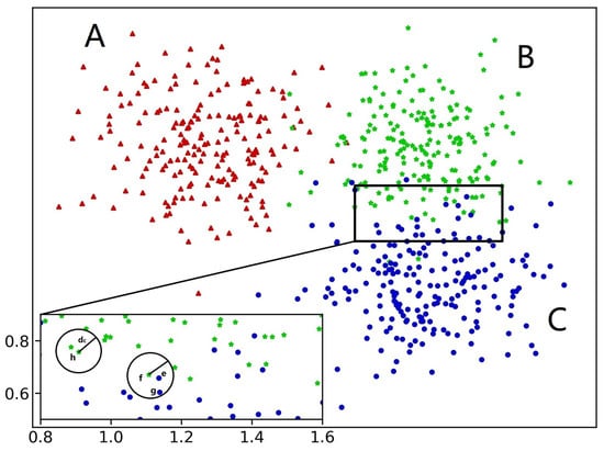
Figure 3.
Example of border points and density reachable.
Based on the concept of density reachable, we can build a graph model for all cluster centers. The cluster centers are the nodes of the graph. If both two centers are density-directly-reachable, they have a connected edge. We can calculate all connected components using the graph model based on the DFS algorithm and merging the connected clusters. As shown in the example in Figure 3, three candidate centers are selected using (7). Let , , and represent the centers of cluster A, B, and C, respectively. Then, we can build a graph model with three nodes, , , and . If clusters B and C are density reachable, then and have an edge. If clusters A and B are not density reachable, then and have no edge. Then, applying the DFS algorithm on this graph model, we can obtain a connected component with two nodes, and . Therefore, clusters B and C can be merged into one.
Based on the above improvements, we can use the improved DPC algorithm to cluster and obtain the cluster label comH.
3.4. Training the Classifier with Core-Set
The advantage of classification algorithms is their high accuracy, but some data points identified by category labels need to be used as a training set. Marking labels manually is a time-consuming task. Clustering algorithms do not need labeled data. However, without providing labels, the learned model will not be accurate enough. The method detailed in Section 3.2 and Section 3.3 provides a batch of labeled data. We can use these data to train the classifier, and then the classifier will determine to which cluster each missing feature data point belongs.
3.4.1. Distance Measurement of Incomplete Data Points
To calculate the K nearest neighbors of the incomplete data point , we should first know how to calculate the distance between data points with missing features. The partial distance (PDS) of incomplete data was proposed in [29]. The distance is calculated according to the visible part of the data point and then multiplied by a factor calculated by the number of missing dimensions. Datta proposed the use of the FWPD [30] distance to directly calculate the distance of incomplete data points and directly applied the FWPD distance to the K-means clustering algorithm to deal with incomplete datasets. However, this method cannot handle incomplete data with an arbitrary shape. FWPD distance is the weighted sum of two terms: the first is the observed distance of two data points, and the second is a penalty term. The penalty term is a weighted sum of the penalty coefficients of all missing dimensions, and the FWPD distance is a weighted sum of the observed distance and the penalty term. It is denoted by and calculated as follows:
where is the observed distance of data points and and S is the set of all feature dimensions. and are the sets of feature dimensions that can be observed by and , respectively. belongs to , which is the number of data points in with the observed values of the lth feature. Obviously, if a feature observed in most samples is missing in a specific sample, this weighting scheme will impose a greater penalty. On the other hand, if the missing feature is not observed in many other samples, a smaller penalty will be imposed. Utilizing the FWPD distance, we can calculate the K nearest complete neighbors of the missing data point and then use the mean value of the corresponding dimension of the K neighbors to impute the missing feature.
3.4.2. Training Classifier
Definition 5
(Core set of a cluster). The core set of a cluster , denoted by , is defined as:
The core set of a cluster contains data points that have a relatively higher local density in the cluster, meaning it can better represent the distribution of the cluster. Using these points as a training set can lead to obtaining a higher-accuracy classifier. A core set is selected from the clustering results of , then the core set is fed to a proper classification model (such as SVM). When the trained classifier is obtained, the classifier can be applied to classify the imputed missing feature data points. The final clustering result is obtained by combining the labels of and the labels of the imputed missing data assigned by the classifier.
3.5. Main Steps of DPC-INCOM
Algorithm 1 provides a summary of the proposed DPC-INCOM.
| Algorithm 1 DPC-INCOM. |
|
3.6. Complexity Analysis
In this section, we measure the computational complexity of the proposed algorithm.The complexity of the entire process is the sum of the complexities of the two stages: DPC clustering in and imputation and classification in . Suppose the dataset has N points and is divided into a complete part with points and an incomplete part with points. In Stage 1, the time complexity of Algorithm 2 depends on the following aspects: (a) calculating the distance between points (); (b) sorting the distance vector of each point (); (c) calculating the cutoff distance (); (d) calculating the local density with the nearest neighbors(); (e) calculating the distance for each point (); (f) selecting initial cluster centers and assigning each remaining point to the nearest point with a higher density (); (g) calculating the border points of each cluster (); (h) calculating the border density of each cluster and merge density-reachable clusters (). Therefore, the complexity of Stage 1 is , which is same as that of basic DPC [11]. In Stage 2, the time complexity depends on the following aspects: (a) calculating the FWPD distance between the incomplete points and the complete points (); (b) imputing all the incomplete points using K2 nearest neighbors ; (c) selecting a core set from the complete points ; (d) training a SVM [33] classifier with core set . When the dataset is large, the complexity can be reduced by switching to an appropriate classifier. The above analysis demonstrates that the overall time complexity of the proposed algorithm is .
| Algorithm 2AKdensityPeak. |
|
4. Experiments and Results
4.1. Dataset
The proposed algorithm was evaluated based on three synthetic datasets and six widely used UCI (http://archive.ics.uci.edu/ml/datasets.php accessed on 24 December 2021) datasets: Iris, Landsat, PenDigits, Seeds, Vote, and Wine. Table 2 provides the details of the datasets.
Table 2.
Datasets used in our experiments.
These nine datasets originally had no missing features. In total, 60% of the samples in each dataset were randomly selected as a complete dataset with no missing data, and the others were selected as an incomplete part. We calculated the total missing number using the missing ratio, then randomly generated enough missing feature positions according to the missing number, noted the positions of the missing features in the missing matrix, and then deleted the features at the corresponding positions according to the missing matrix. The overall missing ratios of the matrices created were 5%, 10%, 15%, 20%, and 25% to affect the performance of the algorithms to varying degrees. The last column in Table 2 indicates the range of missing value in the dataset, which is the product of missing ratio, the number of samples, and dimensions. For example, 200–1000 missing values exist in the five-cluster (synthetic) dataset, which is . Each method was implemented ten times on these edited datasets, and the average of the results was employed to evaluate the performance in avoiding the negative effect of the accidental. We also uploaded the incomplete datasets to GitHub (https://github.com/gaokunnanjing/AK_densitypeak_imcom.git/accessed on 24 December 2021).
The five-cluster dataset (https://scikit-learn.org/stable/modules/generated/sklearn.datasets.make_blobs.html accessed on 24 December 2021), Flame [34], and Twomoons (https://scikit-learn.org/stable/modules/generated/sklearn.datasets.make_moons.html accessed on 24 December 2021) are synthetic two-dimensional datasets. The rest of the datasets were downloaded from the UCI Repository. PenDigits contains hand-written digits with 10,992 samples for 10 classes. The Landsat dataset consists of multi-spectral values of pixels in 3 × 3 neighborhoods in a satellite image, with 2000 samples in 6 classes.
4.2. Compared Algorithm
We compared the proposed clustering method with several commonly used imputation methods, including mean imputation (DPC + Mean), KNN imputation (DPC + KNN), and EM imputation (DPC + EM). In addition, we compared these with the recently proposed dynamic K-means imputation (DK) [28] and the previous three methods.
4.3. Experiment Settings
In our experiment, we assumed that the actual number of clusters was pre-specified. The clustering performance of each algorithm is evaluated by the widely used clustering accuracy (ACC), normalized mutual information (NMI) [35] and Fowles mallows index (FMI) [36]. The algorithms were implemented in Python and run on a Windows laptop with a 2.8 GHz processor and 16 GB of main memory.
4.4. Experimental Results
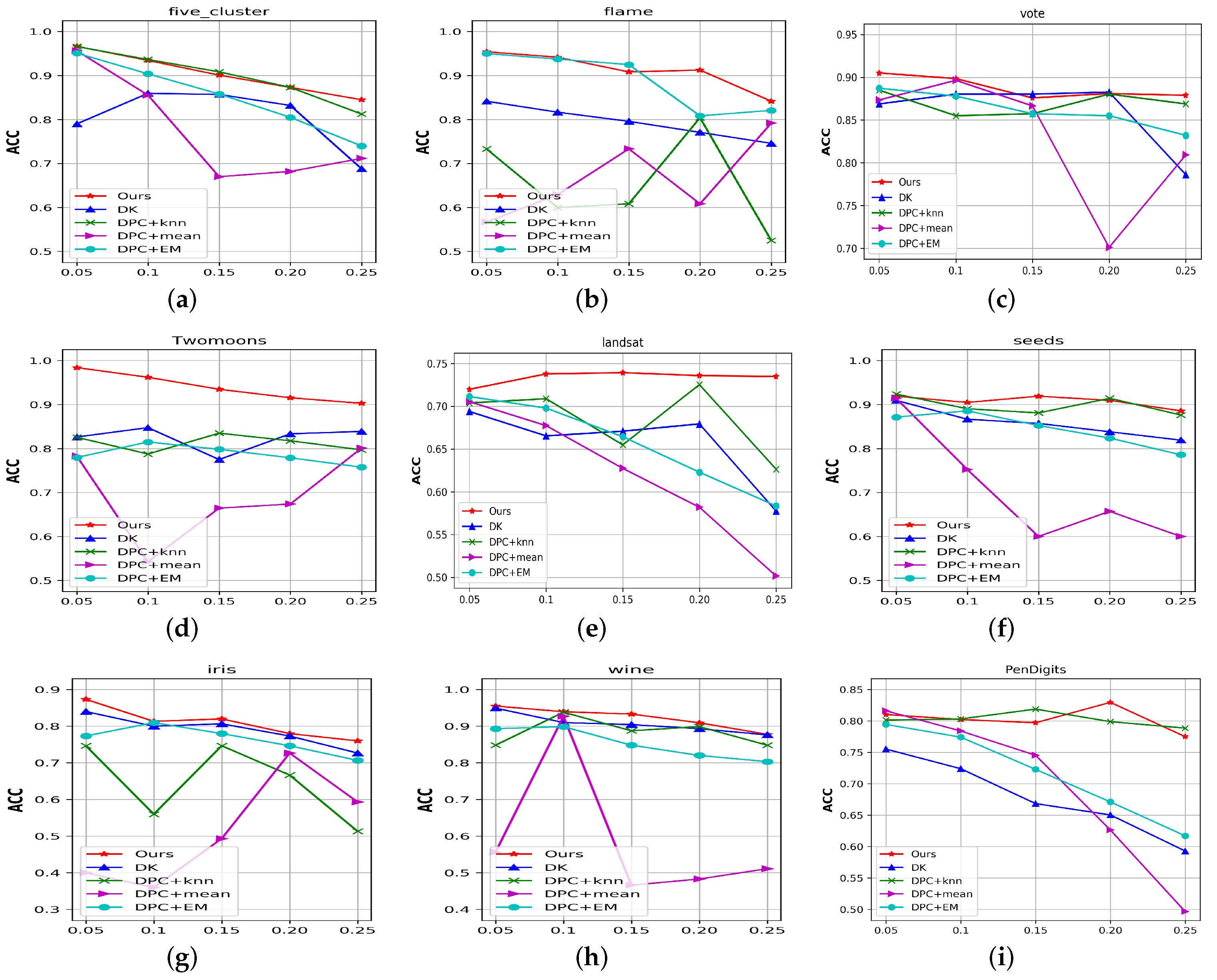
Figure 4 compares the ACC of the above algorithms on all the datasets with different missing data ratios. Figure 5 presents the NMI (left part) and FMI (right part) compared to the above algorithms with 25% missing ratios for all the datasets. We also report the aggregated performance metrics (ACC, NMI, and FMI) in Table 3, where the best results are indicated in bold. From these results, we observed the following:
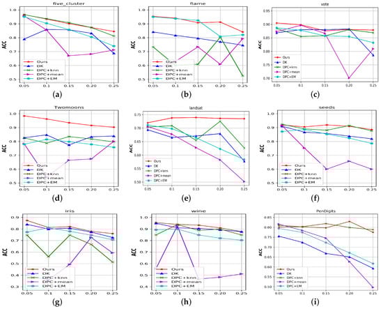
Figure 4.
The ACC of the compared algorithms for different missing data ratios for nine benchmark datasets. (a) Five-cluster. (b) Flame. (c) Vote. (d) Twomoons. (e) Landsat. (f) Seeds. (g) Iris. (h) Wine. (i) PenDigits.
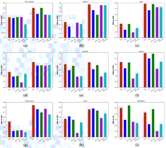
Figure 5.
The NMI and FMI of the compared algorithms with 25% missing data on nine benchmark datasets.(a) Five-cluster. (b) Flame. (c) Vote. (d) Iris. (e) Landsat. (f) Seeds. (g) Twomoons. (h) Wine. (i) PenDigits.
Table 3.
Comparison of the aggregated ACC, NMI, and FMI on nine benchmark datasets.
(1) Our proposed algorithm significantly outperformed the existing imputation-based methods. Taking the aggregated results as examples, our algorithm outperformed the best imputation-based method (DPC + KNN) by 0.5%, 39.3%, 2.1%, 25.1%, 7.2%, 1.1%, 15.7%, 4.2%, and 7.6% in terms of ACC. From Figure 5, setting the missing ratios to 25%, and taking Flame, Iris, Landsat, and Twomoons as examples, our algorithm outperformed DPC + KNN by 46.2%, 9.6%, 8.2%, and 21.2% in terms of FMI. Sometimes, imputation-based methods produced comparatively good performance, but once they were affected by the aggregation phenomenon, they provided poor clustering results. Conversely, our algorithm always performed stably. These results validated the effectiveness of the proposed algorithm.
(2) Although the recently proposed DK algorithm achieved a fairly good performance, the DPC model can handle data with arbitrary shapes. Taking the aggregated results on the Flame, Landsat, Twomoons, and PenDigits datasets as examples, the proposed algorithm outperformed DK by 14.9%, 11.6%, 14.0%, and 19.4% in terms of ACC, respectively. We found that the NMI and FMI trends are similar to those in Figure 5. These results showed the advantages of the proposed algorithm over DK.
(3) As the missing ratio increases, we observed that the performance of the simple imputation-based DPC algorithm (DPC + Mean) suddenly declined significantly. Because the imputed data points gather in some areas and form some high-density areas, if their density is higher than the original center, wrong centers may be selected, resulting in poor clustering performance. Complex imputation methods (such as KNN) also experience certain issues when performing the aggregation of imputed points, resulting in poor clustering results. Figure 4b–e,g illustrates this type of situation.
(4) Our algorithm uses DPC as the basic clustering model; it can handle data with arbitrary shapes better than K-means, fuzzy C-Means, and hierarchical clustering. When dealing with incomplete data, we utilize a classifier to learn what DPC learned from complete data to solve the aggregation problem caused by the imputation-based DPC model. Therefore, the proposed algorithm can work better for situations where there are incomplete data.
4.5. Discussion of Scenarios with High Missing Data Ratios
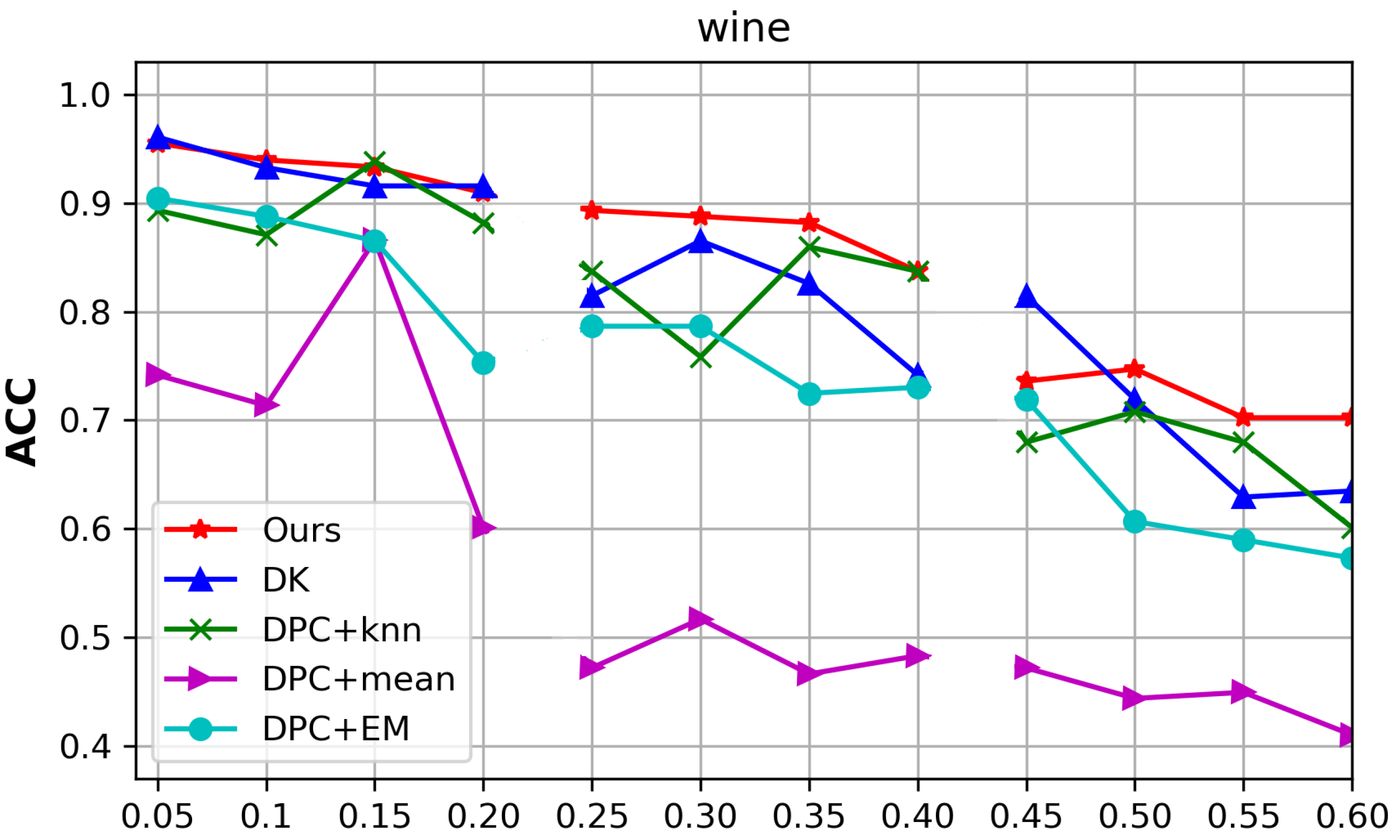
Experiments were conducted on the Wine dataset in a scenario with high missing data ratios. When the total missing ratios were 5–20%, 25–40%, and 45–60%, we selected 60%, 40%, and 20% of the samples as the complete parts, respectively, and randomly deleted values in the remaining 40%, 60%, and 80% of samples, respectively, to generate the incomplete part. The experimental results are shown in Figure 6, which shows that when the missing ratio was less than 40%, the proposed algorithm performed well. When the missing ratio varied from 40% to 60%, the clustering performance of the proposed algorithm showed a sudden drop. Theoretically, we assumed that the distribution of the whole dataset was the same as that of the complete part. Therefore, as long as there are enough representative points in the complete part, the classifier is able to achieve a good distribution of the whole dataset from the clustering results obtained in Stage 1. When the number of samples in the complete part dropped to 20%, the complete part could not represent the distribution of the whole dataset; thus, the clustering performance of the proposed algorithm decreased sharply.
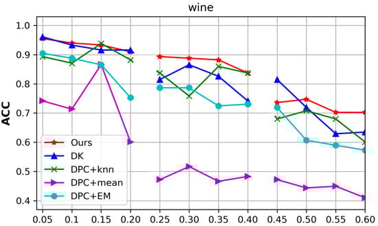
Figure 6.
The ACC of the compared algorithms with the variation in the missing data ratios and complete parts of the Wine dataset.
5. Conclusions
This paper proposed a method that involves combining clustering with classification in two stages: First, the improved DPC model is used to cluster the data points of the complete part and obtain samples with labels. Second, some representatives of these labeled samples are selectd to train a classifier and classify data points with missing features. Our algorithm effectively extends the DPC algorithm to incomplete data. Extensive experiments were conducted on synthetic and UCI datasets to prove the effectiveness of our algorithm, which outperformed the best imputation-based method (DPC + KNN) by up to 39.3% in terms of the ACC on all nine datasets. However, the proposed algorithm needs a sufficient number of representative data points, which often cannot be obtained for many datasets in the real world. In the future, we plan to select more representative data points from the missing data points with fewer missing dimensions to improve the performance of the algorithm.
Author Contributions
Conceptualization, methodology, formal analysis, data curation, software, and writing—original draft, K.G.; resources, supervision, validation, writing—review and editing, W.Q.; writing—review and editing, H.A.K. All authors have read and agreed to the published version of the manuscript.
Funding
This research was funded by the National Natural Science Foundation of China, grant 61572194.
Institutional Review Board Statement
Not applicable.
Informed Consent Statement
Not applicable.
Data Availability Statement
Publicly available datasets were analyzed in this study. This data can be found here: [http://archive.ics.uci.edu/ml/datasets.php] (accessed on 24 December 2021).
Conflicts of Interest
The authors declare no conflict of interest.
References
- Gan, G.; Ma, C.; Wu, J. Data Clustering: Theory, Algorithms, and Applications; Society for Industrial and Applied Mathematics, American Statistical Association: Alexandria, VA, USA, 2007. [Google Scholar]
- Ankerst, M.; Breunig, M.; Kriegel, H.P.; Ng, R.; Sander, J. Ordering points to identify the clustering structure. In Proceedings of the ACM International Conference on Management of Data SIGMOD, Vancouver, BC, Canada, 9–12 June 2008; p. 99. [Google Scholar]
- Han, J.; Kamber, M.; Pei, J. Data Mining: Concepts and Techniques, 3rd ed.; Morgan Kaufmane: Burlington, MA, USA, 2011. [Google Scholar]
- Jain, A. Data clustering: 50 years beyond k-means. Pattern Recognit. Lett. 2010, 31, 651–666. [Google Scholar] [CrossRef]
- Hartigan, J.A.; Wong, M.A. Algorithm AS 136: A k-means clustering algorithm. J. R. Stat. Soc. Ser. C Appl. Stat. 1979, 28, 100–108. [Google Scholar] [CrossRef]
- Suganya, R.; Shanthi, R. Fuzzy c-means algorithm—A review. Int. J. Sci. Res. Publ. 2012, 2, 1. [Google Scholar]
- Wang, K.; Zhang, J.; Li, D.; Zhang, X.; Guo, T. Adaptive affinity propagation clustering. arXiv 2008, arXiv:0805.1096. [Google Scholar]
- Ouyang, M.; Welsh, W.J.; Georgopoulos, P. Gaussian mixture clustering and imputation of microarray data. Bioinformatics 2004, 20, 917–923. [Google Scholar] [CrossRef]
- Ester, M.; Kriegel, H.P.; Sander, J.; Xu, X. A density-based algorithm for discovering clusters in large spatial databases with noise. In Proceedings of the Kdd, Portland, OR, USA, 2–4 August 1996; Volume 96, pp. 226–231. [Google Scholar]
- Xue, Z.; Wang, H. Effective density-based clustering algorithms for incomplete data. Big Data Min. Anal. 2021, 4, 183–194. [Google Scholar] [CrossRef]
- Rodriguez, A.; Laio, A. Clustering by fast search and find of density peaks. Science 2014, 344, 1492. [Google Scholar] [CrossRef] [Green Version]
- Du, M.; Ding, S.; Jia, H. Study on density peaks clustering based on k-nearest neighbors and principal component analysis. Knowl.-Based Syst. 2016, 99, 135–145. [Google Scholar] [CrossRef]
- Yaohui, L.; Zhengming, M.; Fang, Y. Adaptive density peak clustering based on K-nearest neighbors with aggregating strategy. Knowl.-Based Syst. 2017, 133, 208–220. [Google Scholar] [CrossRef]
- Jiang, J.; Chen, Y.; Meng, X.; Wang, L.; Li, K. A novel density peaks clustering algorithm based on k nearest neighbors for improving assignment process. Phys. A Stat. Mech. Its Appl. 2019, 523, 702–713. [Google Scholar] [CrossRef]
- Cao, L.; Liu, Y.; Wang, D.; Wang, T.; Fu, C. A novel density peak fuzzy clustering algorithm for moving vehicles using traffic radar. Electronics 2020, 9, 46. [Google Scholar] [CrossRef] [Green Version]
- Chen, Y.; Hu, X.; Fan, W.; Shen, L.; Zhang, Z.; Liu, X.; Li, H. Fast density peak clustering for large scale data based on kNN. Knowl.-Based Syst. 2020, 187, 104824. [Google Scholar] [CrossRef]
- Lin, J.L.; Kuo, J.C.; Chuang, H.W. Improving Density Peak Clustering by Automatic Peak Selection and Single Linkage Clustering. Symmetry 2020, 12, 1168. [Google Scholar] [CrossRef]
- Shi, Z.; Ma, D.; Yan, X.; Zhu, W.; Zhao, Z. A Density-Peak-Based Clustering Method for Multiple Densities Dataset. ISPRS Int. J. Geo-Inf. 2021, 10, 589. [Google Scholar] [CrossRef]
- Nikfalazar, S.; Yeh, C.H.; Bedingfield, S.; Khorshidi, H. Missing data imputation using decision trees and fuzzy clustering with iterative learning. Knowl. Inform. Syst. 2020, 62, 2419–2437. [Google Scholar] [CrossRef]
- Mostafa, S.M.; Eladimy, A.S.; Hamad, S.; Amano, H. CBRG: A Novel Algorithm for Handling Missing Data Using Bayesian Ridge Regression and Feature Selection Based on Gain Ratio. IEEE Access 2020, 8, 216969–216985. [Google Scholar] [CrossRef]
- Ma, Z.; Liu, Z.; Zhang, Y.; Song, L.; He, J. Credal Transfer Learning With Multi-Estimation for Missing Data. IEEE Access 2020, 8, 70316–70328. [Google Scholar] [CrossRef]
- Mostafa, S.M. Missing data imputation by the aid of features similarities. Int. J. Big Data Manag. 2020, 1, 81–103. [Google Scholar] [CrossRef]
- Dinh, D.T.; Huynh, V.N.; Sriboonchitta, S. Clustering mixed numerical and categorical data with missing values. Inform. Sci. 2021, 571, 418–442. [Google Scholar] [CrossRef]
- Donders, A.R.T.; Van Der Heijden, G.J.; Stijnen, T.; Moons, K.G. A gentle introduction to imputation of missing values. J. Clin. Epidemiol. 2006, 59, 1087–1091. [Google Scholar] [CrossRef]
- Dixon, J.K. Pattern recognition with partly missing data. IEEE Trans. Syst. Man Cybernet. 1979, 9, 617–621. [Google Scholar] [CrossRef]
- Dempster, A.P.; Laird, N.M.; Rubin, D.B. Maximum likelihood from incomplete data via the EM algorithm. J. R. Stat. Soc. Ser. B Methodol. 1977, 39, 1–22. [Google Scholar]
- Zhang, Y.; Li, M.; Wang, S.; Dai, S.; Luo, L.; Zhu, E.; Zhou, H. Gaussian Mixture Model Clustering with Incomplete Data. ACM Trans. Multimedia Comput. Commun. Appl. TOMM 2021, 17, 1–14. [Google Scholar] [CrossRef]
- Wang, S.; Li, M.; Hu, N.; Zhu, E.; Hu, J.; Liu, X.; Yin, J. K-means clustering with incomplete data. IEEE Access 2019, 7, 69162–69171. [Google Scholar] [CrossRef]
- Hathaway, R.J.; Bezdek, J.C. Fuzzy c-means clustering of incomplete data. IEEE Trans. Syst. Man Cybernet. Part B Cybernet. 2001, 31, 735–744. [Google Scholar] [CrossRef] [Green Version]
- Datta, S.; Bhattacharjee, S.; DaSs, S. Clustering with missing features: A penalized dissimilarity measure based approach. Mach. Learn. 2018, 107, 1987–2025. [Google Scholar] [CrossRef] [Green Version]
- Friedman, N.; Geiger, D.; Goldszmidt, M. Bayesian network classifiers. Mach. Learn. 1997, 29, 131–163. [Google Scholar] [CrossRef] [Green Version]
- Bishop, C.M. Neural Networks for Pattern Recognition; Oxford University Press: Oxford, UK, 1995. [Google Scholar]
- Jakkula, V. Tutorial on Support Vector Machine (svm); School of EECS, Washington State University: Washington, DC, USA, 2006; p. 37. [Google Scholar]
- Fu, L.; Medico, E. FLAME, a novel fuzzy clustering method for the analysis of DNA microarray data. BMC Bioinform. 2007, 8, 1–15. [Google Scholar] [CrossRef]
- Strehl, A.; Ghosh, J. Cluster Ensembles—A Knowledge Reuse Framework for Combining Multiple Partitions. J. Mach. Learn. Res. 2002, 3, 583–617. [Google Scholar]
- Jolliffe, I.T.; Morgan, B.J.T. A Method for Comparing Two Hierarchical Clusterings: Comment. J. Am. Stat. Assoc. 1983, 78, 580. [Google Scholar] [CrossRef]


Publisher’s Note: MDPI stays neutral with regard to jurisdictional claims in published maps and institutional affiliations. |
© 2022 by the authors. Licensee MDPI, Basel, Switzerland. This article is an open access article distributed under the terms and conditions of the Creative Commons Attribution (CC BY) license (https://creativecommons.org/licenses/by/4.0/).