Abstract
This study proposes a Disturbance-improved Model-free Adaptive Prediction Control (DMFAPC) algorithm for a discrete-time nonlinear system with time delay and disturbance. The algorithm is shown to have good robustness. On the one hand, the Smith predictor is used to predict the output at a future time to eliminate the time delay in the system; on the other hand, an attenuation factor is introduced at the input to effectively eliminate the measurement disturbance. The proposed algorithm is a data-driven control algorithm that does not require the model information of the controlled system; it only requires the input and output data. The convergence of the DMFAPC is analyzed. Simulation results confirm the effectiveness of this algorithm.
1. Introduction
Discrete-time nonlinear systems with time delay widely exist in the complex industrial production process, such as power systems, water turbine regulating systems, and cement calciner outlet temperature systems [1,2,3]. When a time delay exists, the current control input needs to be fed back to the system output after a certain delay. At the same time, due to the influence of uncertain external interference, the phenomenon often occurs in a nonlinear system [4]. If the system is subjected to external disturbance, the controller cannot suppress in a timely and targeted manner; the control system is prone to overshooting, and the adjustment time will be relatively long, resulting in severe system instability. Therefore, aimed at the discrete-time nonlinear system, the solution of time delay and external disturbance problems is the subject of a lot of research.
Conventional control algorithms such as Smith predictive control [5], the Dahlin algorithm [6], and related improved algorithms [7,8] theoretically solve the control problem of systems with time delay. Most algorithms depend on the precise mathematical model of the controlled plant. However, industrial process systems are highly complex, and it is difficult to establish accurate models and use traditional control algorithms for such systems. In addition, there are a large number of Input/Output (I/O) data in actual process which can accurately reflect the information of the controlled plant. Therefore, the application of data-driven approaches to nonlinear systems with time delay and disturbance has attracted considerable attention.
At present, the existing data-driven control algorithms mainly include the virtual reference feedback setting algorithm [9], iterative algorithm [10], adaptive dynamic programming [11], lazy learning control algorithm [12], and the Model Free Adaptive Control (MFAC) algorithm [13]. Among them, the MFAC algorithm, a typical data-driven control algorithm, has the advantage of requiring a small amount of calculation and having strong adaptability; it has been studied deeply in theory and widely used in practice in, for example, polymerization reaction processes [14], automatic parking systems [15], traffic control [16], and so on.
The MFAC algorithm has been studied for systems with disturbance and time delay. In [17], it is proposed that an improved MFAC algorithm using the Smith predictor to estimate the system output and a tracking differentiator is employed to obtain the differential signal in the predictor. Reference [18] designs a MFAC-PID cascade control system with a dead zone based on PID control with strong anti-interference and MFAC. While the anti-interference ability of the controlled system is improved, a hybrid controller combining MFAC with slide control is proposed to ensure the control accuracy, and a sliding mode compensation item is added on the basis of model-free adaptive control to enhance the robustness of the system [19]. MFAC is also proposed on the basis of the improved discrete extended observer [20]. The disturbance is estimated by the discrete state extended observer, and the controlled system then set the controller to improve the control performance. Research on data-driven robustness has achieved significant results. MFAC based on multi-adaptive observers by considering the interference in multiple input channels is proposed in [21]. Reference [22] studies the data-driven control system of combined spacecraft by considering the influence of disturbances. In [23], a novel MFAC algorithm is proposed to mitigate disturbance and data packet loss. Reference [24] analyzes the multi-input multi-output quadrotor model, combined with the auto-disturbance rejection technology with MFAC, and proposes a new approach to mitigate the disturbance.
The above-mentioned studies only considered the control algorithm in the case of time delay or disturbance. Few existing studies have attempted to mitigate the time delay and disturbance simultaneously. In fact, in the industrial control process, most of the time delays and disturbances exist simultaneously. In addition, the predictive control algorithm is an effective means to deal with time delay and disturbance; it can apply the future data to design the controller. References [25,26] make a new attempt for the discrete-time nonlinear system and propose a class of model-free adaptive predictive controls (MFAPC). However, for the discrete-time nonlinear system with time delay and disturbance simultaneously, the corresponding theory of MFAPC has not been established.
Based on this, a disturbance-improved model-free adaptive predictive control (DMFAPC) is proposed for discrete-time nonlinear systems with time delays and disturbances by introducing a Smith prediction technique and attenuation factor.
The contributions of the paper are as follows:
- (1)
- A class of discrete-time nonlinear system is dynamically linearized by Form Dynamic Linearization Technology, so that the current dynamic process of the controlled plant can be described by a virtual equivalent dynamic linearization model.
- (2)
- A novel DMFAPC controller is designed. The Smith prediction technique and attenuation factor are introduced to deal with the time delay and measurement disturbance in the controlled plant effectively. In addition, the prediction mechanism further enhances the robustness of the proposed controller.
- (3)
- A strict mathematical derivation and convergence proof of the DMFAPC are given, to verify the validity of the algorithm from the view of mathematical analysis. From the simulation view, the effectiveness of the proposed algorithm is verified by a series of numerical simulations.
2. Disturbance-Improved Model-Free Adaptive Prediction Control Scheme
2.1. Dynamic Linearization of Time-Delay System with Disturbance
A single-input single-output discrete-time nonlinear perturbed system with time delay can be expressed as
where and represent the output and input at time k, respectively, represents the delay time of the system, represents the measured output at time k, represents the bounded measurement disturbance at time k, and are two unknown positive integers representing the order of the system, and is an unknown nonlinear function.
Hypothesis 1.
System (1) is measurable and controllable for the input and output.
Hypothesis 2.
Except for limited time points, the partial derivative of the nonlinear functionwith respect to the control input signalof the system is continuous.
Hypothesis 3.
Except for limited time points, system (1) is a generalized Lipschitz system [27].
2.1.1. Dynamic Linearization
Lemma 1.
If the nonlinear system (1) satisfies Hypotheses 1–3, when, there must be a pseudo-partial derivativethat satisfies, and this pseudo-partial derivative is bounded.
According to the above-mentioned lemma, the compact dynamic linearization model of system (1) can be expressed as
The analysis of model (3) shows that the control input at time k − 1 will yield an unknown output . Therefore, Equation (3) cannot be directly used for controller design.
In [17], it suggested that when the system parameters and structure vary slowly with time. Seen in the Figure 1, can be used instead of to complete the function of the Smith predictor.
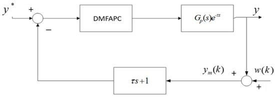
Figure 1.
System structure.
Hence, Equation (3) can be expressed as
where is the derivative of .
In Figure 1, is the transfer function of the controlled plant.
2.1.2. Tracking Differentiator
To obtain the derivative output by Equation (4), this study employs a second-order tracking differentiator [28]. The second-order tracking differentiator can be described as
For the input signal , the system will generate two output signals and ; is the tracking signal of and is the differential of . In Equation (11), T is the sampling step, and h and r are the filter factor and speed factor, respectively.
2.2. Design of Controller for Time-Delay System with Disturbance
Based on Equations (2) and (4), the N-step forward prediction equation of the system is expressed as follows:
where N is the number of predictive steps and is the constant of the control time domain.
Let
Equation (13) can be abbreviated as
The following input criterion function is considered:
where is the expected output of the system at time k + i.
Let
Equation (15) can be rewritten as
By substituting Equation (14) into Equation (16), we take the partial derivative of and make it equal to 0; then, the following control law can be obtained:
The control amount at the current moment is
where .
After the analysis, the tracking error of Equation (17) is found to be bounded but not convergent. Therefore, the following improved algorithm with an attenuation factor is proposed:
Using a parameter estimation algorithm symmetrical to the control algorithm, we get
The DMFAPC is constructed as follows:
The definitions of can be determined by the following equations:
where
The whole controller implementation process described using the pseudocode is summarized in Algorithm 1: Pseudocode of the disturbance-improved model-free adaptive prediction control.
| Algorithm 1 Disturbance-Improved Model-Free Adaptive Prediction Control |
| Begin set initial parameter and desired output fork = 1: N calculate using Equation (21) if or end define calculate using Equation (23) if end for j = calculate using Equation (25) if or end end assign the parameter calculate using Equation (27). calculate using Equation (28) calculate the control input error according to the controlled system, calculate the control output end |
2.3. Stability Analysis
Hypothesis 4.
For a given bounded expected output signal, there is always a boundedsuch that under this control input signal, the output of the system is equal to.
Hypothesis 5.
After a sufficiently large moment,, the pseudo-partial derivative of the system, andonly at limited moments.
Hypothesis 6.
The system measurement disturbance w(k) is a random signal, and its statistical characteristics are.
Hypothesis 7.
When m≥0, the measurement disturbance d(k + m) is not related to y(k), u(k − 1),, i.e.,
Theorem 2.
Under the condition that Hypotheses 1–7 are satisfied, the DMFAPC algorithm is applied to the time-delay system with disturbance, given by Equations (1) and (2):
The output tracking error of the system is monotonically convergent, and .
The closed-loop system is BIBO stable, i.e., the output sequence and the input sequence are bounded.
Proof.
First, we prove that the pseudo-partial derivative converges. □
From Equation (22), when or , is obviously bounded.
In other cases, is defined as the estimation error of the pseudo-partial derivative. By subtracting from both sides of the estimation algorithm given by Equation (21), the following equation can be obtained:
By taking the absolute value of both sides of Equation (30) simultaneously, the following equation can be obtained:
Suppose that ; then, Equation (31) can be rewritten as
The first part of the right-hand side of Equation (32) contains constants ; hence, the following equation is established:
According to Equation (33),
and
where is the upper bound of . By combining Equation (34) with Equation (35), it can be seen that is bounded. Hence, is also bounded.
It is also known from Equations (21)–(27) that is bounded.
The following proves that the tracking error is 0, i.e., the input and output sequences are bounded.
The tracking error of the system is defined as . Let , ,.
When ,
As is a positive semi-definite matrix, if > 0, and are positive definite matrices. In addition, , is the adjoint matrix of the matrix , and is the algebraic remainder of . Then, the following equation is established:
Since is bounded at any time k and all are bounded, Equation (37) is bounded and is not correlated with k.
There are constants and ,. Therefore, from Equation (36),
Suppose that there is a small positive number ∂, . Then, Equation (38) can be rewritten as
When k is an even number, according to Equation (39), we get
From Equation (40),. Further, according to Equation (40), when k is an odd number, can be proved. Hence, we have .
As is a bounded constant, the sequence is bounded.
Using Equations (28) and (29), we get
where is a bounded constant.
Therefore, we have
Equation (42) shows that the input sequence is bounded, and the proof is complete.
3. Simulations
3.1. Simulation under Different Data-Driven Algorithms
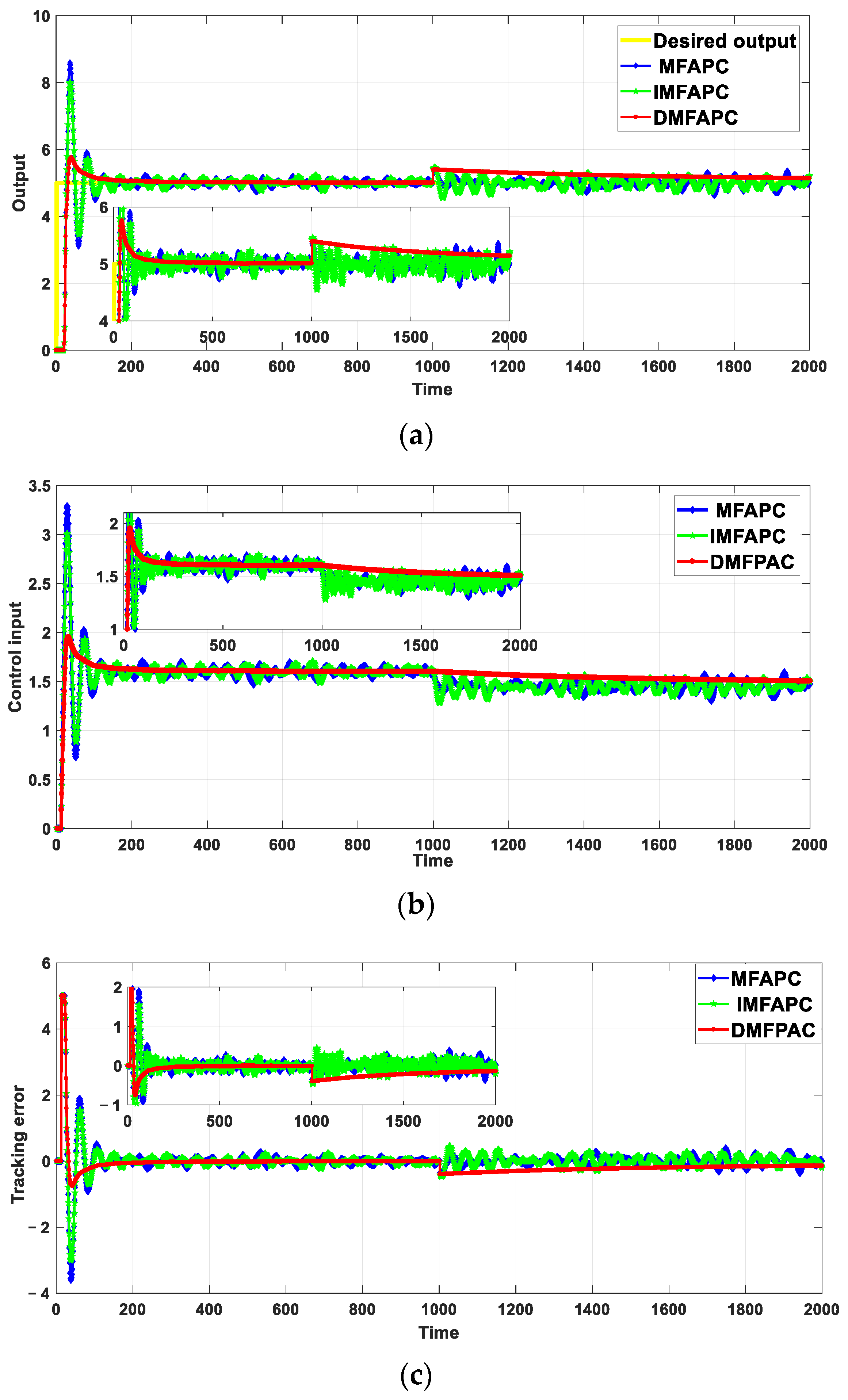
Aimed at discrete-time nonlinear systems with time delays and disturbances, a traditional Model-free Adaptive Predictive Control (MFAPC) and Improved Model-free Adaptive Predictive Control (IMFAPC) [3] are selected to compare with the proposed DMFAPC to verify the effectiveness of the algorithm.
Given a general discrete-time nonlinear system with time delay [17]
The disturbance of the above-mentioned system is set as a random measurement disturbance expressed as . The expected value of the output is set to 5 and the delay time is 9. The parameters are set to , , , , , and . Further, for the MFAPC, IMFAPC, and DMFAPC are 100, 100, and 1, respectively. The simulation results are shown in Figure 2.

Figure 2.
Performance of different algorithms. (a) The output performance of different algorithms; (b) The input performance of different algorithms; (c) The tracking error of different algorithms.
It can be seen from Figure 2 that while the measurement disturbances exist, neither MFAPC nor IMFAPC can eliminate the disturbance, resulting in a bounded measurement error. When the controlled plant changes, there will be oscillation. The proposed DMFAPC algorithm is obviously superior to the other and can eliminate the simultaneous delay and disturbance in the system more effectively. The DMFAPC still maintains good robustness even when the controlled plant changes. In order to further verify the effectiveness of the algorithm, three kinds of error evaluation indexes as Mean Absolute Error (MAE), Mean Square Error (MSE), and Root Mean Square Error (RMSE) are selected for comparison, as shown in the Table 1.

Table 1.
Error evaluation.
3.2. Simulation under Different Disturbances
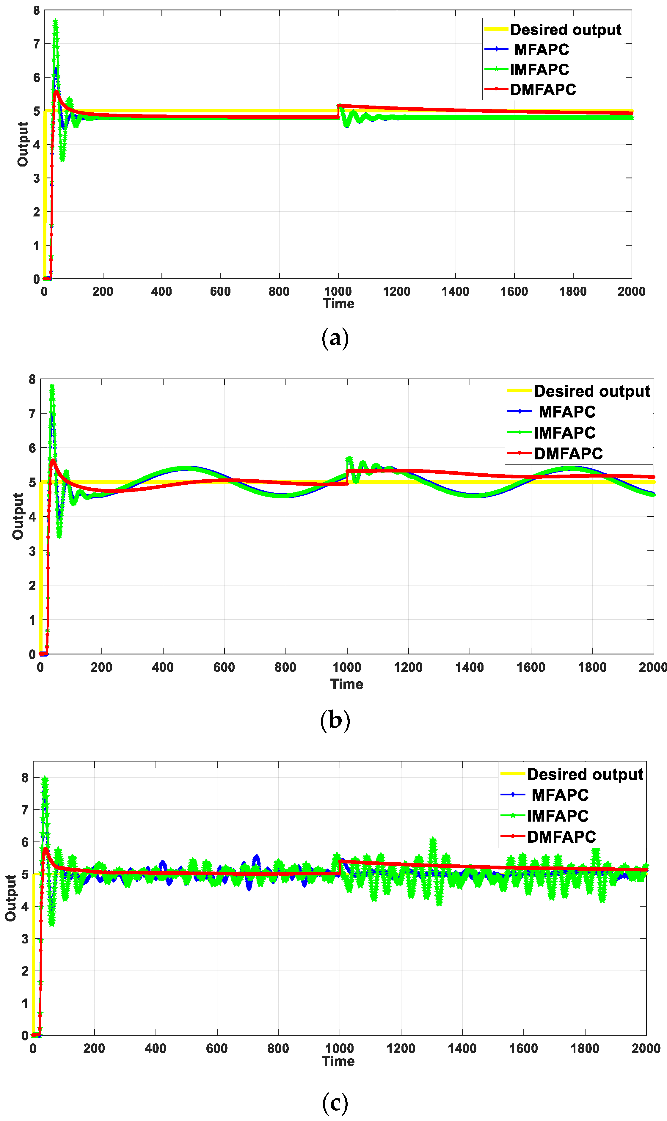
In order to verify the influence of different disturbances on tracking effect, three disturbance signals are selected for comparative experiment, constant disturbance , random disturbance and sinusoidal disturbance , respectively. The simulation results are shown in Figure 3.

Figure 3.
Tracking performance with different algorithms. (a) Tracking performance with . (b) Tracking performance with . (c) Tracking performance with .
It shows that MFAPC and IMFAPC have strong robustness when the disturbance is constant, and can automatically eliminate the influence. When the disturbance is random or sinusoidal, MFAPC and IMFAPC are very susceptible to perturbations. By comparison, DMFAPC can eliminate the influence of disturbance and has strong robustness no matter how the disturbance changes.
3.3. Simulation under Different Time Delay
Figure 4 shows the performance of DMFAPC algorithm under the influence between three different time delays.
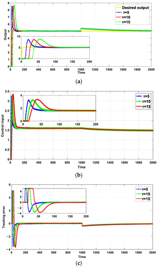
Figure 4.
Control performance with different time delay. (a) The output performance of the DMFAPC. (b) The input performance of the DMFAPC. (c) The tracking error of the DMFAPC.
As can be seen from the Figure 4, the larger the time delay τ is, the longer the system takes to reach stability. The larger the overshoot and tracking error are, and the more energy is needed to control input. Through the analysis of the simulation, it can be found that the DMFAPC algorithm r has faster control speed and better control effect for the discrete-time nonlinear system with time delay and disturbance.
4. Conclusions
This study combined the concept of the Smith predictor with model-free adaptive prediction control based on the dynamic linearization algorithm with a compact format and proposed a new DMFAPC algorithm for a single-input single-output perturbed system with time delay. In addition, the convergence and stability of this algorithm were proved via theoretical analysis. The controller of the algorithm is simple, the parameter adjustment is convenient, and no model is required. For discrete-time nonlinear systems with time delay and disturbance, compared with other algorithms from different views, the proposed DMFAPC has a better suppression effect on measurement disturbance and good robustness. In addition, it also shows a faster control speed for time delay phenomenon.
In the future, on one hand, we will extend the DMFAPC to the multiple input and multiple output nonlinear system. On the other hand, we will try to combine DMFAPC with the multi-agent consensus coordination algorithms to solve the vehicle control problem at road intersections.
Author Contributions
Conceptualization, H.J. and S.L.; methodology, Y.W. (Yulin Wang) and S.L.; validation, S.L., L.F.; formal analysis, H.J. and Y.W. (Yuzhou Wei); writing—original draft preparation, Y.W. (Yulin Wang) and Y.W.(Yuzhou Wei); writing—review and editing, Y.W. (Yuzhou Wei) and H.J; supervision, H.J and S.L.; project administration, L.F.; funding acquisition, L.W. All authors have read and agreed to the published version of the manuscript.
Funding
This work is supported by Beijing Municipal Natural Science Foundation under Grant 4204098 and 4212035, National Natural Science Foundation (NNSF) of China under Grant 61903004 and 61803036, North China University of Technology YuYou Talent Training Program, North China University of Technology Scientific Research Foundation, Beijing Information Science and Technology University Scientific Research Classified Development Program under Grant 2121YJPY214, Beijing Municipal Great Wall Scholar Program under Grant CIT&TCD20190304.
Conflicts of Interest
The author declares that there are no conflict of interest.
References
- Fridman, E. Introduction to Time-Delay Systems: Analysis and Control; Birkhauser: Basel, Switzerland, 2014. [Google Scholar]
- Mahmoud, M.S. Robust Control and Filtering for Time-Delay Systems; Marcel Dekker: New York, NY, USA, 2000. [Google Scholar]
- Wang, L.; Zhu, Y.; Zhong, W. An improved model free adaptive predictive control for time delay systems. Control. Eng. 2021, 2, 382–387. [Google Scholar]
- Xu, J.; Yu, X.; Qiao, J. Hybrid Disturbance Observer-Based Anti-Disturbance Composite Control with Applications to Mars Landing Mission. IEEE Trans. Syst. Man Cybern. Syst. 2021, 51, 2885–2893. [Google Scholar] [CrossRef]
- Gao, J.; Sun, Q. Enhanced PID Controllers Design Based on Modified Smith Predictor Control for Unstable Process with Time Delay. Math. Probl. Eng. 2014, 2014, 521460. [Google Scholar]
- Teng, F.; Ledwich, G.; Tsoi, A. Extension of the Dahlin-higham Controller to Multivariable Systems with Time Delays. Int. J. Syst. Sci. 1994, 25, 337–350. [Google Scholar] [CrossRef]
- Zhang, H.; Hu, J.; Bu, W. Research on Fuzzy Immune Self-Adaptive PID Algorithm Based on New Smith Predictor for Networked Control System. Math. Probl. Eng. 2015, 2015, 343416. [Google Scholar] [CrossRef]
- Chen, G.; Liu, D.; Mu, Y. A Novel Smith Predictive Linear Active Disturbance Rejection Control Strategy for the First-Order Time-Delay Inertial System. Math. Probl. Eng. 2021, 2021, 5560123. [Google Scholar]
- Campi, M.; Mavaresi, S. Direct nonlinear control design: The virtual reference feedback tuning (VRFT) approach. IEEE Trans. Automat. Contr. 2006, 51, 14–27. [Google Scholar] [CrossRef]
- Radac, M.; Precup, R.; Petriu, E.; Preitl, S. Iterative data-driven tuning of controllers for nonlinear systems with constraints. IEEE Trans. Ind. Electron. 2014, 61, 6360–6368. [Google Scholar] [CrossRef]
- Zhang, Q.; Zhao, D.; Wang, D. Event-based robust control for uncertain nonlinear systems using adaptive dynamic programming. IEEE Trans. Neural Netw. Learn. Syst. 2016, 29, 37–50. [Google Scholar] [CrossRef]
- Garcia, E.; Feldman, S.; Gupta, M.; Srivastava, S. Completely Lazy Learning. IEEE Trans. Knowl. Data Eng. 2010, 22, 1274–1285. [Google Scholar] [CrossRef]
- Hou, Z. The Parameter Identification, Adaptive Control and Model Free Learning Adaptive Control for Nonlinear Systems; Northeastern University: Shenyang, China, 1994. [Google Scholar]
- Zhu, Y.; Hou, Z. Controller dynamic linearisation-based model-free adaptive control framework for a class of nonlinear system. IET Control. Theory Appl. 2015, 9, 1162–1172. [Google Scholar] [CrossRef]
- Xu, D.; Shi, Y.; Ji, Z. Model free adaptive discrete-time integral sliding mode constrained control for autonomous 4WMV parking systems. IEEE Trans. Ind. Electron. 2017, 65, 834–843. [Google Scholar] [CrossRef]
- Jin, M.; Lee, J.; Tsagarakis, N. Model-free robust adaptive control of humanoid robots with flexible joints. IEEE Trans. Ind. Electron. 2017, 64, 1706–1715. [Google Scholar] [CrossRef]
- Jin, S.; Hou, Z. An Improved Model-free Adaptive Control for A Class of Nonlinear Large-lag Systems. IET Control. Theory Appl. 2008, 25, 623–626. [Google Scholar]
- Gu, Z.; Sun, Y.; Zhong, Y. Model-free adaptive control for dead zone. Therm. Power Gener. 2015, 44, 86–90. [Google Scholar]
- Pan, X.; Xian, B. Model-free adaptive robust control design for a small unmanned helicopter. IET Control. Theory Appl. 2017, 34, 1171–1178. [Google Scholar]
- Hui, Y.; Chi, R. Iterative extended state observer-based data driven optimal iterative learning control. IET Control. Theory Appl. 2018, 35, 129–136. [Google Scholar]
- Xu, D.; Jiang, B.; Shi, P. A novel model-free adaptive control design for multivariable industrial processes. IEEE Trans. Ind. Electron. 2014, 61, 6391–6398. [Google Scholar] [CrossRef]
- Han, G.; Guangfu, M.; Yueyong, L. Data-driven model-free adaptive attitude control of partially constrained combined spacecraft with external disturbances and input saturation. Chin. J. Aeronaut. 2019, 32, 1281–1293. [Google Scholar]
- Pu, X. Research on Robustness of Data Driven Model-Free Adaptive Control and Learning Control; Beijing Jiaotong University: Beijing, China, 2015. [Google Scholar]
- Liu, S.; Hou, Z.; Zhang, X. Model-Free Adaptive Control Method for a Class of Unknown MIMO Systems with Measurement Noise and Application to Quadrotor Aircraft. IET Control. Theory Appl. 2020, 14, 2084–2096. [Google Scholar] [CrossRef]
- Jin, S.; Hou, Z.; Chi, R.; Bu, X. Model free adaptive predictive control approach for phase splits of urban traffic network. In Proceedings of the 2016 Chinese Control and Decision Conference (CCDC), Yinchuan, China, 28–30 May 2016. [Google Scholar]
- Hou, Z.; Liu, S.; Tian, T. Lazy-learning-based data-driven model-free adaptive predictive control for a class of discrete-time nonlinear systems. IEEE Trans. Neural Netw. Learn. Syst. 2017, 28, 1914–1928. [Google Scholar] [CrossRef] [PubMed]
- Hou, Z.; Jin, S. Model Free Adaptive Control: Theory and Applications; CRC Press: Boca Raton, FL, USA, 2013. [Google Scholar]
- Han, J. From PID to Active Disturbance Rejection Control. IEEE Trans. Ind. Electron. 2009, 56, 900–906. [Google Scholar] [CrossRef]

Publisher’s Note: MDPI stays neutral with regard to jurisdictional claims in published maps and institutional affiliations. |
© 2021 by the authors. Licensee MDPI, Basel, Switzerland. This article is an open access article distributed under the terms and conditions of the Creative Commons Attribution (CC BY) license (https://creativecommons.org/licenses/by/4.0/).