Article

On Dynamic Investigations of Cournot Duopoly Game: When Firms Want to Maximize Their Relative Profits

Department of Statistics and Operations Research, College of Science, King Saud University, P.O. Box 2455, Riyadh 11451, Saudi Arabia
Symmetry 2021, 13(12), 2235; https://doi.org/10.3390/sym13122235
Submission received: 18 October 2021 / Revised: 9 November 2021 / Accepted: 15 November 2021 / Published: 23 November 2021
(This article belongs to the Special Issue Chaotic Systems and Nonlinear Dynamics)

Abstract

:
This paper studies a Cournot duopoly game in which firms produce homogeneous goods and adopt a bounded rationality rule for updating productions. The firms are characterized by an isoelastic demand that is derived from a simple quadratic utility function with linear total costs. The two competing firms in this game seek the optimal quantities of their production by maximizing their relative profits. The model describing the game’s evolution is a two-dimensional nonlinear discrete map and has only one equilibrium point, which is a Nash point. The stability of this point is discussed and it is found that it loses its stability by two different ways, through flip and Neimark–Sacker bifurcations. Because of the asymmetric structure of the map due to different parameters, we show by means of global analysis and numerical simulation that the nonlinear, noninvertible map describing the game’s evolution can give rise to many important coexisting stable attractors (multistability). Analytically, some investigations are performed and prove the existence of areas known in literature with lobes.

1. Introduction

Oligopoly market structure has been characterized by a few interdependent firms that collectively dominate the market. It has been thoroughly studied and analyzed in economic dynamics and game theory. The duopoly one on which the current manuscript focuses on has been considered a particular case from oligopoly, but with only two firms (or competitors). In duopoly, each firm simultaneously chooses its decision or strategy based on its own actions and those taken by its competitor. Literature has reported several studies in duopoly games focusing either in static and dynamic cases. There have been many studies in handling dynamic cases because they have possessed several dynamic behaviors, which have attracted many researchers. Such dynamic behaviors have included different types of bifurcations, peculiar basins of attraction for chaotic attractors and multistability phenomena. In addition, there were different utility functions that were the core of many studies in such games. For instance, there was the most popular utility function, known Cobb–Douglas utility. It is a particular functional form of production function that has been widely adopted to represent the technological relationship between the amounts of two or more inputs and the amount of output that can be produced by those inputs. Furthermore, there was the constant elasticity of substitution (CES) utility, Singh and Vives utility, and others. These utilities and their properties can be found in the literature ([1,2,3,4,5,6,7,8,9,10]).
The current paper adopts a nonlinear utility function that can be considered as a particular case of the Singh and Vives utility. Applying Lagrange first-order conditions on the adopted utility gives rise to isoelastic demand functions for both firms, and they are the same as those given by Cobb–Douglas utility [1]. Due to the complex dynamic characteristics of duopoly models literature has reported many interesting results about Nash equilibrium point of these games and consequently many researchers have been attracted. We report here some related works and results in this direction. For instance, a game of differentiated products with two competitors whose decision variables are different, known as Cournot–Bertrand duopoly game, has been investigated in [11]. More studies on seeking the optimality of production by competing firms have been introduced and discussed in ([12,13,14]). In [15], Tremblay and Tremblay studied a Cournot–Bertrand duopoly game with differentiated products and their studies were concentrated on Nash equilibrium and its stability in static phase. A Cournot–Bertrand game depending on a theoretical framework has been introduced in [16]. In [17], Naimzada et al. have introduced a Cournot–Bertrand model that is described by a two-dimensional discrete linear map. Their focus was on the dynamic characteristics of Nash equilibrium points and the bifurcation types by which it became unstable. Conversely, studying and modeling the evolution of such games require some rules of adjustments by which competing firms can adjust their updating productions. Indeed, the literature has reported several studies that adopted many adjustment approaches used for that purpose. Bounded rationality mechanism has been ranked first in such studies and has been deeply adopted in the modeling process. It has been considered as a gradient-rule mechanism as it depends on the marginal profit and requires competing firms to carry out an estimation on it whether it increases or decreases, so firms can update their output production next time period. Besides this mechanism, there were other useful approaches adopted in many studies in the literature like, for example, the tit-for-tat rule and the approximation of local monopolistic mechanism ([18,19,20,21,22,23,24,25,26,27]).
Adopting the bounded rationality rule and a nonlinear quadratic utility function that is considered as a particular case form Singh and Vives utility a Cournot duopoly game that belongs to those discussed above is introduced in the current manuscript. Indeed, the adopted utility function by firms in this paper is different than that introduced and used in [28]. Unlike several studies in the literature, the two competing firms in this game want to maximize their relative profits. Our analysis performed here includes local and global investigations on the map’s dynamics around Nash equilibrium point in the asymmetric case. This includes the types of bifurcations by which it can be unstable and routes to chaos can be raised. Discussion on the coexistence of multiple stable attractors and attracting sets whose attractive basins structures are peculiar because of the coexistence of the so-called lobes is analyzed. Our discussion shows that Nash point can be destabilized due to flip and Neimark–Sacker bifurcations also confirms the coexistence of lobes as the game’s map has owns a focal point makes both denominator and nominator of the map vanish. Furthermore, we prove that this map is noninvertible and is of type Z 1 Z 3 , where the phase plane is divided by the region Z i , i refers to the number of preimages. The symmetric case when equal parameters values are adopted does not possess important dynamic characteristics like those obtained in this manuscript for the asymmetric case. For this reason, our analysis here is focused on the later case. In addition, one has to highlight that the current studies in this paper differ from those obtained in [29]. The inverse demand function in this paper is isoelastic while it is linear in [29]. The relative profits to be maximized is more general than those adopted in [29]. Furthermore, the current paper analyzes the dynamics with asymmetric parameters as both competing firms adopt different marginal cost and different speed of adjustment parameters. Moreover, the current paper considers [30] as a special case but with the same adjustment mechanism. Interesting readers are advised to see other similar studies in literature [31].
The summary of the paper can be set as follows. The game’s model and its analytical structure is given in Section 2. In Section 3, local analysis on the stability of the unique equilibrium point (Nash point) is studied both analytically and numerically. In Section 4, the main results in this paper on global analysis which discusses some peculiar basins of attraction and lobes are presented. Finally, the findings are summarized.

2. The Model

Let us suppose the utility function given by,
U = Q Q 2 = q 1 + q 2 ( q 1 + q 2 ) 2
This quadratic utility is concave and Q = q 1 + q 2 and q i , i = 1 , 2 represents total supply of quantities to market. We study here a game of two competing firms (or players) that produce the quantity q i , i = 1 , 2 . Both players adopt the above utility in economic market. It is easy to see that 2 U q 1 q 2 = 2 0 and that is to say the marginal utility of goods does not depend on each, and hence U is homogeneous utility function. Using p 1 q 1 + p 2 q 2 = 1 as a budget constraint, then one can obtain the optimization problem given below.
M a x U = q 1 + q 2 ( q 1 + q 2 ) 2 s . t p 1 q 1 + p 2 q 2 = 1
where p i > 0 , i = 1 , 2 denotes a price for good q i , i = 1 , 2 . The optimization problem (2) gives (see Appendix A)
p = 1 Q
Now, profits can be,
π i ( q 1 , q 2 ) = p i q i C ( q i ) = 1 Q c i q i , i = 1 , 2
where C i ( q i ) = c i q i , i = 1 , 2 denotes quantity’s cost. The marginal cost ( C i ( q i ) q i = c i , i = 12 , ) is non-negative constant. Let us assume the two competing firms want to maximize their relative profits given by
φ 1 = π 1 α 1 π 2 , φ 2 = π 2 α 2 π 1
where π i , i = 1 , 2 denotes firm’s i own profit and the parameter α i , i = 1 , 2 where 1 < α i < 1 can be directly interpreted as a measure of altruism. It can also be explained as firms’ care of relative performance. If α i = 0 , i = 1 , 2 it means firms give care to their own profits only. Substituting (4) in (5) one gets,
φ 1 = q 1 α 1 q 2 Q c 1 q 1 + α 1 c 2 q 2 , φ 2 = q 2 α 2 q 1 Q c 2 q 2 + α 2 c 1 q 1
So the marginal relative profits φ i q i , i = 1 , 2 are
φ 1 q 1 = ( 1 + α 1 ) q 2 Q c 1 , φ 2 q 2 = ( 1 + α 2 ) q 1 Q c 2
Now, firms want to maximize their relative profits, and this requires them to know the characteristics of the market where competition is carried out. In order to know these characteristics, firms should know complete information on the market and their competitors, but this is impossible. To overcome that, firms estimate their updating production next period of time based on the sign of the marginal relative profits, φ i q i , i = 1 , 2 . If φ i q i > 0 then firms increase their production next period of time, otherwise they decrease productions or become naive. The rule by which they estimate production is called bounded rationality rule and is given by [32]
q i ( t + 1 ) = q i ( t ) + k i ( q i ) φ i q i ; i = 1 , 2
Let us suppose that k i ( q i ) = ν i q i ; i = 1 , 2 where ν i > 0 , i = 1 , 2 is a speed of adjustment parameter. Given that one gets q i ( t + 1 ) q i ( t ) q i ( t ) φ i q i and, hence, the relative production is directly proportional to marginal relative profit. Properties of this rule are studied and reported elsewhere ([26,27,28,30]). Substituting (7) in (8), one obtains a two-dimensional discrete map describing the game’s repetition as follows.
T q 1 , q 2 : q 1 ( t + 1 ) = q 1 ( t ) + ν 1 q 1 ( t ) ( 1 + α 1 ) q 2 Q c 1 , q 2 ( t + 1 ) = q 2 ( t ) + ν 2 q 2 ( t ) ( 1 + α 2 ) q 1 Q c 2
where t = 0 , 1 , 2 , . . . refers to time periods. Setting T q 1 , q 2 = q 1 , q 2 in (9) one gets a unique fixed point that is Nash equilibrium and the map is not defined at ( 0 , 0 )
e * = c 2 ( 1 + α 2 ) ( 1 + α 1 ) 2 c 1 ( 1 + α 2 ) + c 2 ( 1 + α 1 ) 2 , c 1 ( 1 + α 1 ) ( 1 + α 2 ) 2 c 1 ( 1 + α 2 ) + c 2 ( 1 + α 1 ) 2
which is positive point.

3. Local Stability

The stability of the above Nash point is given in the following propositions where their proofs are given in Appendix A.
Proposition 1.
The Nash point e * is locally asymptotically stable if the following condition is satisfied,
c 1 c 2 ν 1 ν 2 < 4 c 1 c 2 ( 1 + α 2 ) ν 2 + ( 1 + α 1 ) ν 1 c 1 ( 1 + α 2 ) + c 2 ( 1 + α 1 ) < 4 + c 1 c 2 ν 1 ν 2
Proposition 2.
The Nash point e * loses its stability due to flip bifurcation only if the following condition is satisfies
4 c 1 c 2 ( 1 + α 2 ) ν 2 + ( 1 + α 1 ) ν 1 c 1 ( 1 + α 2 ) + c 2 ( 1 + α 1 ) > 4 + c 1 c 2 ν 1 ν 2
Proposition 3.
The Nash point e * loses its stability due to Neimark–Sacker bifurcation only if the following condition is satisfied.
4 c 1 c 2 ( 1 + α 2 ) ν 2 + ( 1 + α 1 ) ν 1 c 1 ( 1 + α 2 ) + c 2 ( 1 + α 1 ) < 4 + c 1 c 2 ν 1 ν 2
Now, some numerical experiments are performed to validate the above propositions. Assuming the values, c 1 = 2 , c 2 = 2.5 , α 1 = 0.5 and α 2 = 0.5 , Figure 1a presents the stability region of Nash point and the conditions (12) and (13) where flip and Neimark–Sacker bifurcations are held. It is clear that the Nash equilibrium point can be destabilized by means of either flip or Neimark–Sacker bifurcation. Assuming the values, c 1 = 2 , c 2 = 2.5 , α 1 = 0.5 , α 2 = 0.5 and ν 2 = 0.3 one can see that the condition (13) is satisfied, but Nash point loses its stability due to flip bifurcation when ν 1 0.90566 , as given in Figure 1b. Fixing the previous values including ν 1 = 0.2 Figure 1c shows the flip bifurcation diagram on varying ν 2 and hence Nash point becomes unstable when ν 2 0.903226 , . Conversely, when selecting the values, c 1 = 1 , c 2 = 2 , α 1 = 0.5 , α 2 = 0.5 and ν 2 = 1.29 a Neimark–Sacker bifurcation occurs as shown in Figure 1d. Simulation shows that, at these values of parameters, the Neimark–Sacker takes place when ν 1 1.379679 , 6.461539 and the condition (12) is non-negative while (13) becomes negative. At ν 1 > 6.461539 , both conditions become negative. Figure 1e presents a Neimark–Sacker bifurcation on varying the parameter ν 2 at the set of parameters, c 1 = 1 , c 2 = 2 , α 1 = 0.5 , α 2 = 0.5 and ν 1 = 1.35 . Extra numerical experiments are carried out for values of the parameter ν 1 above its critical point 0.90566 at the set of values, c 1 = 2 , c 2 = 2.5 , α 1 = 0.5 , α 2 = 0.5 and ν 2 = 0.3 . Figure 1f undergoes a period-2 cycle denoted by stars with Nash point denoted by circle at ν 1 = 1.0095 . At ν 1 = 1.0336 , a period-4 cycle is born, and as this parameter increases to 1.0517881 , a two-bands chaotic attractor emerges. Further increasing to ν 1 = 1.0781457 , a one piece chaotic attractor is raised. At another set of values, c 1 = 1 , c 2 = 2 , α 1 = 0.5 , α 2 = 0.5 and ν 2 = 1.29 , Figure 2a shows quasi-periodic dynamic behavior with an attracting closed ring at ν 1 = 1.4568456 . This closed ring is followed by a period-8 cycle at the same set of values, but for ν 1 = 1.4725503 . The figure also shows a two different one piece chaotic attractors at the same set of values, but for ν 1 = 1.5208725 and ν 1 = 1.5408054 , respectively. Simulation shows that different values for α 1 and α 2 can affect the stability region in the ( ν 1 , ν 2 ) -plane. For example, at the sets of parameters values c 1 = 2 , c 2 = 2.5 , α 1 = 0.5 , α 2 = 0.3 and c 1 = 2 , c 2 = 2.5 , α 1 = 0.7 , α 2 = 0.6 the stability region in ( ν 1 , ν 2 ) -plane is reduced.

4. Global Analysis

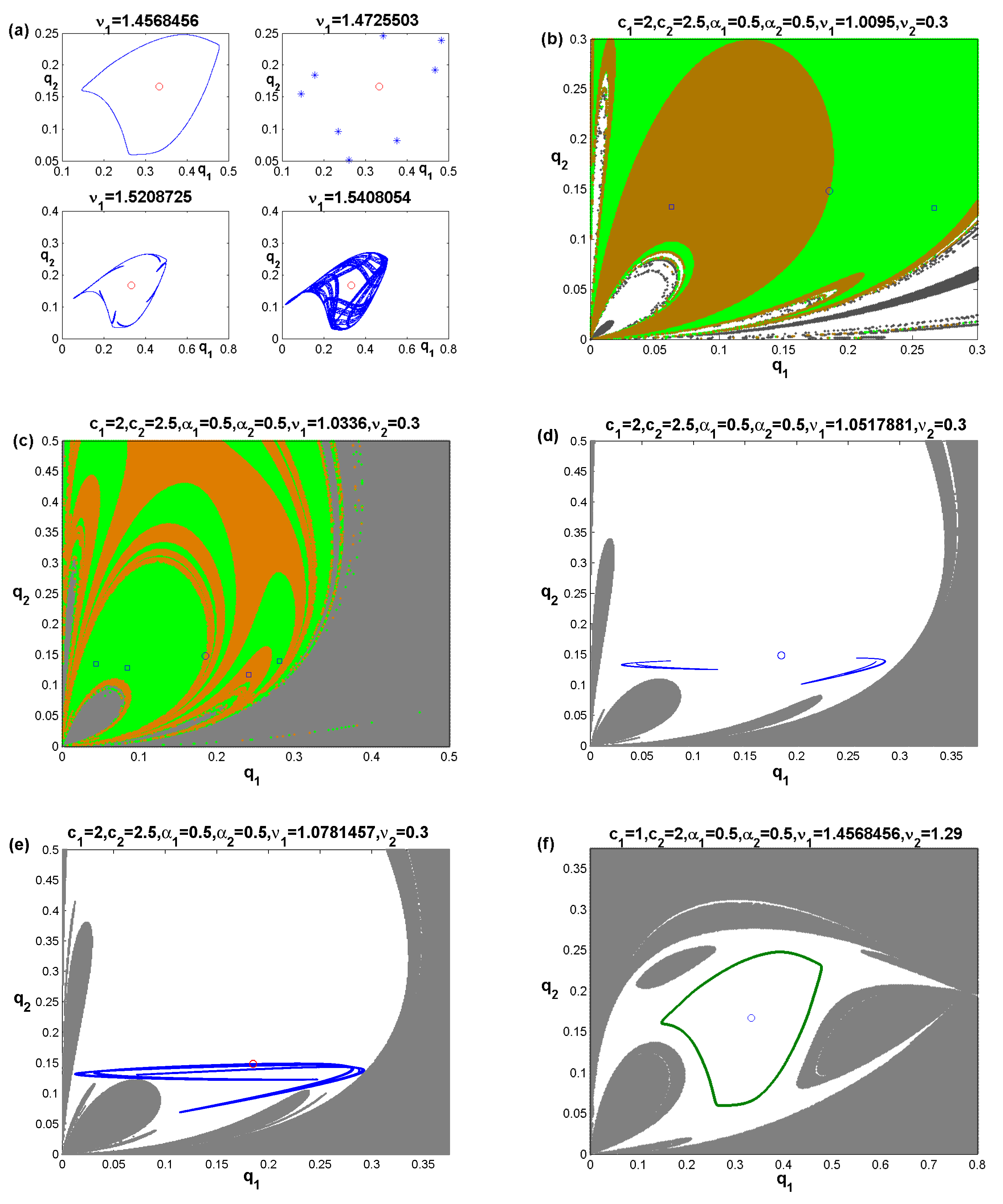
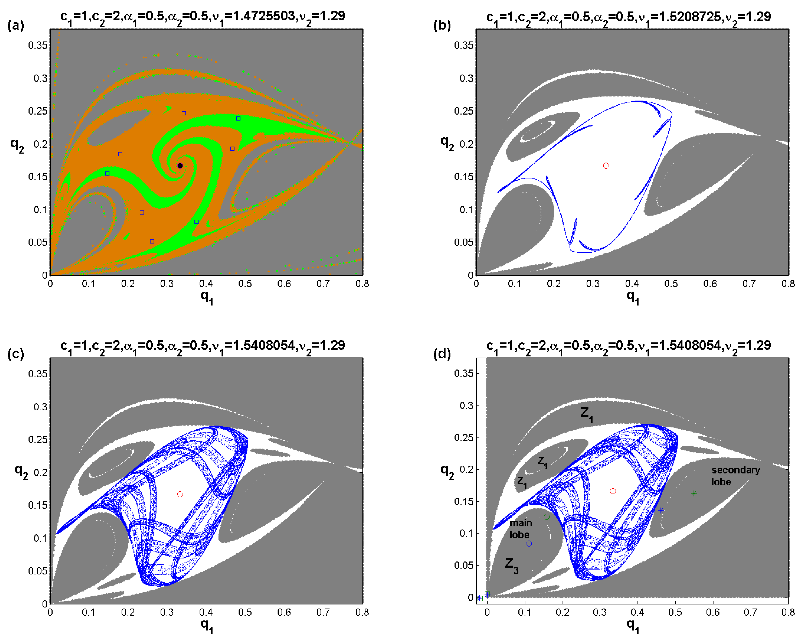
In this section, global analysis about the map’s trajectories are performed. This includes the basins of attraction on some attracting sets and chaotic attractors. Figure 2b shows the basin of attraction for a period-2 cycle with Nash point. This periodic cycle is born at the parameters values, c 1 = 2 , c 2 = 2.5 , α 1 = 0.5 , α 2 = 0.5 , ν 1 = 1.0095 and ν 2 = 0.3 . The attracting domain is plotted by white color, while the dark gray refers to the escaping domain (divergence). The other colors refer to the basin of attraction for Nash and this cycle. It is clear that there are some lobes that are created from the origin point. The reason for creating these lobes is discussed later. Keeping the other parameter values fixed and increasing ν 1 to 1.0336 one gets a period-4 cycle. It is depicted on Figure 2c with Nash and their basins of attraction and is noted that the number of lobes is increased. One can also see that the escaping domain forms a disconnecting set. At ν 1 = 1.0517881 , while the other values are fixed, a two-bands chaotic attractor is raised. Its basin of attraction given in Figure 2d has an attracting domain that contains many lobes from the divergent one (or unfeasible trajectories). Further increasing of ν 1 to 1.0781457 gives rise to a one piece chaotic attractor with lobes form the escaping domain. Conversely, assuming the set of values, c 1 = 1 , c 2 = 2 , α 1 = 0.5 , α 2 = 0.5 , ν 1 = 1.4568456 and ν 2 = 1.29 , Figure 2f shows a dynamic situation of an attracting invariant closed ring with Nash point. One can see that this attractive basin is peculiar and the attracting domain contains lobes and holes from the infeasible one. At these parameters value but for ν 1 = 1.4725503 a successive period-8 cycle is emerged. Its basin of attraction is given in Figure 3a with Nash point. In Figure 2b,c, there are two different chaotic attractors whose attractive basins contain lobes and holes for the same set of parameters values, but for ν 1 = 1.5208725 and ν 1 = 1.5408054 .

4.1. Noninvertible Map

Setting ( q 1 ( t + 1 ) , q 2 ( t + 1 ) ) = ( 0 , 0 ) in T given in (9), one finds
0 = q 1 ( t ) + ν 1 q 1 ( t ) ( 1 + α 1 ) q 2 Q c 1 , 0 = q 2 ( t ) + ν 2 q 2 ( t ) ( 1 + α 2 ) q 1 Q c 2
The algebraic system (14) has only one solution given by,
O 1 = q ˚ 1 , q ˚ 2 , q ˚ 1 = ( 1 + α 1 ) 2 ( 1 + α 2 ) ( 1 c 2 ν 2 ) ν 1 2 ν 2 ν 1 ( 1 + α 1 ) ( 1 c 2 ν 2 ) + ν 2 ( 1 + α 2 ) ( 1 c 1 ν 1 ) 2 q ˚ 2 = ( 1 + α 2 ) 2 ( 1 + α 1 ) ( 1 c 1 ν 1 ) ν 1 ν 2 2 ν 1 ( 1 + α 1 ) ( 1 c 2 ν 2 ) + ν 2 ( 1 + α 2 ) ( 1 c 1 ν 1 ) 2
This means that the origin point possesses only one preimage point and hence it belongs to Z 1 zone. This zone is characterized by only one preimage point. Let us calculate the preimages of any point lies on the vertical axis ( q 1 ( t + 1 ) = 0 , q 2 ( t + 1 ) = q ¯ 0 ). So one has the following algebraic system.
0 = q 1 ( t ) + ν 1 q 1 ( t ) ( 1 + α 1 ) q 2 Q c 1 ,
q ¯ = q 2 ( t ) + ν 2 q 2 ( t ) ( 1 + α 2 ) q 1 Q c 2
From (16) one gets, q 1 = 0 or 0 = 1 c 1 ν 1 + ( 1 + α 1 ) ν 1 q 2 Q and then the following two cases are raised.
Case 1. Substituting q 1 = 0 in (17) gives q 2 = q ¯ 1 c 2 ν 2 and so the point 0 , q ¯ has one preimage point that is O 1 ( 1 ) = 0 , q ¯ 1 c 2 ν 2 .
Case 2. Let 0 = 1 c 1 ν 1 + ( 1 + α 1 ) ν 1 q 2 Q that can be combined with (17) to find
q 1 = ( 1 + α 1 ) ν 1 ν 2 ( 1 + α 2 ) ( c 2 ν 2 1 ) q ¯ ( 1 c 2 ν 2 ) q 2
Substituting (18) in (17) and solve for q 2 one finds
q 2 = q ¯ 1 c 2 ν 2 , q 2 = ( 1 + α 1 ) ν 1 q ¯ ( 1 + α 1 ) ν 1 1 c 2 ν 2 + ( 1 + α 2 ) ν 2 + ( 1 + α 2 ) ( 1 c 2 ν 2 ) ν 2
Substituting (19) in (18) one can get the following two preimages.
O 1 ( 2 ) = 0 , q ¯ 1 c 2 ν 2 , O 1 ( 3 ) = q ˜ 1 , q ˜ 2 , q ˜ 1 = ( 1 + α 1 ) ν 1 q ¯ 1 c 2 ν 2 + ( 1 + α 1 ) ν 1 ( 1 + α 1 ) ν 1 1 c 2 ν 2 + ( 1 + α 2 ) ν 2 + ( 1 + α 2 ) ( 1 c 2 ν 2 ) ν 2 q ˜ 2 = ( 1 + α 1 ) ν 1 q ¯ ( 1 + α 1 ) ν 1 1 c 2 ν 2 + ( 1 + α 2 ) ν 2 + ( 1 + α 2 ) ( 1 c 2 ν 2 ) ν 2
This means the point 0 , q ¯ has three preimages and hence it belongs to Z 3 zone. It is the zone that is characterized by three preimage point. Similarly, one can see that any point in the form p ¯ , 0 has also three preimages. Therefore, any points belonging to the invariant axes q 1 or q 2 will have three preimages except the origin point that has only one preimage point. Furthermore, Nash point belongs to Z 3 zone and Figure 3d shows that the main lobe is also belongs to Z 3 zone and its points has three preimages used to form points of the secondary lobe. Therefore, one can conclude that the phase plane of any attracting set will be divided into Z 1 and Z 3 and hence the game’s map is of type Z 1 Z 3 .

4.2. Focal Point and Lobes

The map (9) can be rewritten as follows.
T q 1 , q 2 : q 1 ( t + 1 ) = q 1 ( t ) + ν 1 q 1 ( t ) N 1 ( q 1 , q 2 ) D ( q 1 , q 2 ) , q 2 ( t + 1 ) = q 2 ( t ) + ν 2 q 2 ( t ) N 2 ( q 1 , q 2 ) D ( q 1 , q 2 )
where, N 1 ( q 1 , q 2 ) = ( 1 + α 1 c 2 ) q 2 c 1 q 1 , N 2 ( q 1 , q 2 ) = ( 1 + α 2 c 2 ) q 1 c 2 q 2 and D ( q 1 , q 2 ) = Q . As one can see, this map is defined in R 2 except the points satisfying the line δ S : q 2 = q 1 and its preimages of any order. Moreover, for q 1 , q 2 δ S one gets only D ( q 1 , q 2 ) = 0 and both N 1 ( q 1 , q 2 ) 0 and N 2 ( q 1 , q 2 ) 0 . Following to [30] this map takes the form 0 / 0 at Q = ( 0 , 0 ) which is called a focal point. The Q = ( x o , y o ) is called a focal point ([30]) if at least one component of the map T becomes in the form 0 / 0 in Q and there exists smooth simple arcs γ ( t ) with γ ( 0 ) = Q such that lim τ 0 T ( γ ( τ ) ) is finite. Additionally, it is cited in ([30]) that for a focal point Q there exists an associated prefocal curve, δ Q that is constructed by all the points mapped into Q by at least one of the inverses of map (21). For the map (21), the prefocal set is defined the prefocal line, δ Q : q 2 = 0 or q 1 = 0 . At the focal point Q one gets the following,
N ¯ 1 , q 1 = N 1 q 1 = c 1 , N ¯ 1 , q 2 = N 1 q 2 = ( 1 + α 1 c 2 ) D ¯ q 1 = D q 1 = 1 , D ¯ q 2 = D q 2 = 1 N ¯ 2 , q 1 = N 2 q 1 = ( 1 + α 2 c 2 ) , N ¯ 2 , q 2 = N 2 q 2 = c 2
and then we have N ¯ 1 , q 2 D ¯ q 1 N ¯ 1 , q 1 D ¯ q 2 = 1 + α 1 + c 1 c 2 , N ¯ 2 , q 2 D ¯ q 1 N ¯ 2 , q 1 D ¯ q 2 = 1 + α 2 that means Q is simple. A simple focal point satisfies, N ¯ 1 , q 2 D ¯ q 1 N ¯ 1 , q 1 D ¯ q 2 0 , N ¯ 2 , q 2 D ¯ q 1 N ¯ 2 , q 1 D ¯ q 2 0 and this means that there exists a correspondence among arcs through the focal Q and points of the prefocal line δ Q and such correspondence is one-to-one.

4.3. Lobes Construction

Though the obtained results above, one can see that some basins of attraction are peculiar due to the emergence of lobes and holes. Figure 2 and Figure 3 present the basins of attraction for some attracting sets and chaotic attractors and as one can see there are lobes and holes that are corresponded to the diverging trajectories that is denoted by B ( ) . There are also some peculiar shapes in these basins which require us to focus on the construction of these lobes. As shown above the game’s map possesses two invariant axes q 1 and q 2 . That is to say,
T 0 , q 2 = 0 , ( 1 c 2 ν 2 ) q 2 , T q 1 , 0 = ( 1 c 1 ν 1 ) q 1 , 0
The two invariant axes are denoted by ω 1 and ω 2 while their preimages are denoted by ω 1 1 and ω 2 1 . Figure 4a shows the basin of attraction for Nash equilibrium only and as one can see that there are no lobes or holes. It can be noted that ω 1 1 separates the basin of attraction of feasible trajectories colored by light gray and infeasible trajectories denoted by red color. In Figure 4b, where the basin of attraction of the chaotic attractor given in Figure 3d is depicted one can see that both this chaotic becomes tangent to both ω 1 1 that intersects ω 2 1 in the preimage point of focal point ( 0 , 0 ) . Furthermore, simulation experiments show that the main lobe whose points belong to Z 3 is formed by real rank-1 preimages of the portions of B ( ) above the prefocal line δ Q : q 2 = 0 or q 1 = 0 issuing from the focal point ( 0 , 0 ) . While the points of secondary lobe issuing from O 1 is formed by points of the main lobe.

5. Conclusions

In this paper, a Cournot duopoly game whose players produce homogeneous goods and are rational has been introduced. The target for those competing firms was to updating their output productions based on maximization of their relative profits. The unique equilibrium point of this game coincides with Nash point and its stability conditions have been obtained. Using local analysis, it has been proved that this point loses its stability through two types of bifurcations, flip and Neimark–Sacker. Because of the structure of game’s map both types of bifurcation have been resulted in for high values of speed reactivity parameters. The map possesses a structure containing components whose nominator and denominator vanish at the origin point (that is characterized as a focal point) that is the reason for creating peculiar shapes of basin of attraction of some attracting sets and chaotic attractors. Discussion of such lobes has shown that they are simple lobes, however, that give rise to such peculiar shapes. These peculiar shapes may be raised due to many reasons such as nonlinearity, noninvertible case, and asymmetric structure of the map or because of adopting the same bounded rationality rule. Furthermore, some numerical experiments have been carried out in the symmetric case and the map’s dynamics was poor in comparison with asymmetric one.
For future studies, heterogeneous players will be studied and the local monopolistic rule will be adopted. This will be applied on economic markets with more than two firms, for example the triopoly case.
...

Funding

This research was funded by King Saud University.

Acknowledgments

Research Supporting Project number (RSP-2021/167), King Saud University, Riyadh, Saudi Arabia.

Conflicts of Interest

The author declares that they have no conflict of interest.

Appendix A

The Lagrange function is given by
L ( q 1 , q 2 , λ ) = U ( q 1 , q 2 ) + λ 1 p 1 q 1 p 2 q 2
whose first-order conditions become
L q 1 = U q 1 λ p 1 = 0 , L q 2 = U q 2 λ p 2 = 0 , L λ = 1 i = 1 2 p i q i
Substituting in the first two equations of (A2) one can get (3).
Proof of Proposition 1.
For the map (9), the Jacobian matrix becomes
J ( q 1 , q 2 ) = 1 + ν 1 ( 1 + α 1 ) q 2 ( q 2 q 1 ) ( q 1 + q 2 ) 3 c 1 ( 1 + α 1 ) q 1 ( q 1 q 2 ) ν 1 ( q 1 + q 2 ) 3 ( 1 + α 2 ) q 2 ( q 2 q 2 ) ν 2 ( q 1 + q 2 ) 3 1 + ν 2 ( 1 + α 2 ) q 2 ( q 1 q 2 ) ( q 1 + q 2 ) 3 c 2
that at e * takes the form
J e * = 1 2 c 1 c 2 ( 1 + α 1 ) ν 1 c 1 ( 1 + α 2 ) + c 2 ( 1 + α 1 ) c 2 ( 1 + α 1 ) c 2 ( 1 + α 1 ) c 1 ( 1 + α 2 ) ν 1 ( 1 + α 2 ) c 1 ( 1 + α 2 ) + c 2 ( 1 + α 1 ) c 1 ( 1 + α 2 ) c 2 ( 1 + α 1 ) c 1 ( 1 + α 2 ) ν 2 ( 1 + α 1 ) c 1 ( 1 + α 2 ) + c 2 ( 1 + α 1 ) 1 2 c 1 c 2 ( 1 + α 2 ) ν 2 c 1 ( 1 + α 2 ) + c 2 ( 1 + α 1 )
The stability of e * is governed by Jury’s conditions
1 T ( J e * ) + det ( J e * ) > 0 , 1 + T ( J e * ) + det ( J e * ) > 0 , 1 det ( J e * ) > 0 ,
where,
T ( J e * ) = 2 2 c 1 c 2 ( 1 + α 1 ) ν 1 + ( 1 + α 2 ) ν 2 c 1 ( 1 + α 2 ) + c 2 ( 1 + α 1 ) , det ( J e * ) = 1 + c 1 c 2 ν 1 ν 2 2 c 1 c 2 ( 1 + α 1 ) ν 1 + ( 1 + α 2 ) ν 2 c 1 ( 1 + α 2 ) + c 2 ( 1 + α 1 )
Substituting (A6) in (A5) we obtain
1 T ( J e * ) + det ( J e * ) = c 1 c 2 ν 1 ν 2 1 + T ( J e * ) + det ( J e * ) = 4 + c 1 c 2 c 1 ( 1 + α 2 ) + c 2 ( 1 + α 1 ) ν 1 ν 2 4 ( 1 + α 2 ) ν 2 4 ( 1 + α 1 ) ν 1 c 1 ( 1 + α 2 ) + c 2 ( 1 + α 1 ) 1 det ( J e * ) = c 1 c 2 c 1 ( 1 + α 2 ) + c 2 ( 1 + α 1 ) ν 1 ν 2 2 ( 1 + α 2 ) ν 2 2 ( 1 + α 1 ) ν 1 c 1 ( 1 + α 2 ) + c 2 ( 1 + α 1 )
Since c i , ν i , i = 1 , 2 are positive, the first condition in (A7) is always nonnegative. Now, letting the other two conditions be nonnegative and then combining them, one obtains
c 1 c 2 ν 1 ν 2 < 4 c 1 c 2 ( 1 + α 2 ) ν 2 + ( 1 + α 1 ) ν 1 c 1 ( 1 + α 2 ) + c 2 ( 1 + α 1 ) < 4 + c 1 c 2 ν 1 ν 2
This completes the proof of Proposition 1. □
Proof of Proposition 2.
Let us suppose that 1 + T ( J e * ) + det ( J e * ) < 0 and 1 det ( J e * ) > 0 . Simple calculations show that
4 c 1 c 2 ( 1 + α 2 ) ν 2 + ( 1 + α 1 ) ν 1 c 1 ( 1 + α 2 ) + c 2 ( 1 + α 1 ) > 4 + c 1 c 2 ν 1 ν 2
and then the proof is completed. □
Proof of Proposition 3.
Let us suppose that 1 + T ( J e * ) + det ( J e * ) > 0 and 1 det ( J e * ) < 0 . Simple calculations show that
4 c 1 c 2 ( 1 + α 2 ) ν 2 + ( 1 + α 1 ) ν 1 c 1 ( 1 + α 2 ) + c 2 ( 1 + α 1 ) < 4 + c 1 c 2 ν 1 ν 2
and then the proof is completed. □

References

  1. Singh, N.; Vives, X. Price and quantity competition in a differentiated duopoly. Rand J. Econ. 1984, 15, 546–554. [Google Scholar] [CrossRef]
  2. Elsadany, A.A. Dynamics of a Cournot duopoly game with bounded rationality based on relative profit maximization. Appl. Math. Comput. 2017, 294, 253–263. [Google Scholar] [CrossRef]
  3. Tuinstra, J. A price adjustment process in a model of monopolistic competition. Int. Game Theory Rev. 2004, 6, 417–442. [Google Scholar] [CrossRef]
  4. Naimzada, A.K.; Raimondo, R. Chaotic congestion games. Appl. Math. Comput. 2018, 321, 333–348. [Google Scholar] [CrossRef]
  5. Ueda, M. Effect of information asymmetry in Cournot duopoly game with bounded rationality. Appl. Math. Comput. 2019, 362, 124535. [Google Scholar] [CrossRef] [Green Version]
  6. Puu, T. Chaos in duopoly pricing. Chaos Solitons Fractals 1991, 1, 573–581. [Google Scholar] [CrossRef]
  7. Askar, S.S.; Al-khedhairi, A. Dynamic investigations in a duopoly game with price competition based on relative profit and profit maximization. J. Comput. Appl. Math. 2020, 367, 112464. [Google Scholar] [CrossRef]
  8. Askar, S.S. On Cournot–Bertrand competition with differentiated products. Ann. Oper. Res. 2014, 223, 81–93. [Google Scholar] [CrossRef]
  9. Askar, S.S. Tripoly Stackelberg game model: One leader versus two followers. Appl. Math. Comput. 2018, 328, 301–311. [Google Scholar] [CrossRef]
  10. Askar, S.S.; Al-Khedhairi, A. Analysis of nonlinear duopoly games with product differentiation: Stability, global dynamics, and control. Discret. Dyn. Nat. Soc. 2017, 2017, 2585708. [Google Scholar] [CrossRef] [Green Version]
  11. Bylka, S.; Komar, J. Cournot-Bertrand mixed oligopolies. In Warsaw Fall Seminars in Mathematical Economics 1975. Lecture Notes in Economics and Mathematical Systems; Łoś, M., Łoś, J., Wieczorek, A., Eds.; Springer: Berlin/Heidelberg, Germany, 1976; Volume 133. [Google Scholar]
  12. Häckner, J. A note on price and quantity competition in differentiated oligopolies. J. Econ. Theory 2000, 93, 233–239. [Google Scholar] [CrossRef] [Green Version]
  13. Zanchettin, P. Differentiated duopoly with asymmetric costs. J. Econ. Manag. Strategy 2006, 15, 999–1015. [Google Scholar] [CrossRef]
  14. Arya, A.; Mittendorf, B.; Sappington, D.E.M. Outsourcing, vertical integration, and price vesus quantity competition. Int. J. Ind. Organ. 2008, 26, 1–16. [Google Scholar] [CrossRef]
  15. Tremblay, C.H.; Tremblay, V.J. The Cournot-Bertrand model and the degree of product differentiation. Econ. Lett. 2011, 111, 233–235. [Google Scholar] [CrossRef]
  16. Askar, S.S. On complex dynamics of cournot-bertrand game with asymmetric market information. Appl. Math. Comput. 2021, 393, 125823. [Google Scholar] [CrossRef]
  17. Naimzada, A.K.; Tramontana, F. Dynamic properties of a Cournot-Bertrand duopoly game with differentiated products. Econ. Model. 2012, 290, 1436–1439. [Google Scholar] [CrossRef]
  18. Ma, J.; Sun, L.; Hou, S.; Zhan, X. Complexity study on the Cournot-Bertrand mixed duopoly game model with market share preference. Chaos 2018, 28, 023101–023110. [Google Scholar] [CrossRef]
  19. Ahmed, E.; Hegazi, A.S.; Elettreby, M.F.; Askar, S.S. On multi-team games. Phys. A Stat. Mech. Appl. 2006, 369, 809–816. [Google Scholar] [CrossRef]
  20. Ahmed, E.; Elettreby, M.F. Controls of the complex dynamics of a multi-market Cournot model. Econ. Model. 2014, 37, 251–254. [Google Scholar] [CrossRef]
  21. Peng, Y.; Lu, Q. Complex dynamics analysis for a duopoly Stackelberg game model with bounded rationality. Appl. Math. Comput. 2015, 271, 259–268. [Google Scholar] [CrossRef]
  22. Tramontana, F. Heterogeneous duopoly with isoelastic demand function. Econ. Model. 2010, 27, 350–357. [Google Scholar] [CrossRef]
  23. Tanimoto, J. Evolutionary Games with Sociophysics; Springer: Berlin/Heidelberg, Germany, 2019. [Google Scholar]
  24. Tanimoto, J. Fundamentals of Evolutionary Game Theory and Its Applications; Springer: Berlin/Heidelberg, Germany, 2015. [Google Scholar]
  25. Tanimoto, J. Mathematical Analysis of Environmental System; Springer: Berlin/Heidelberg, Germany, 2014. [Google Scholar]
  26. Zhong, W.; Kokubo, S.; Tanimoto, J. How is the equilibrium of continuous strategy game different from that of discrete strategy game? Biosystems 2012, 107, 88–94. [Google Scholar] [CrossRef] [PubMed]
  27. Kokubo, S.; Wang, Z.; Tanimoto, J. Spatial reciprocity for discrete, continuous and mixed strategy setups. Appl. Math. Comput. 2015, 259, 552–568. [Google Scholar] [CrossRef]
  28. Wang, H.; Ma, J. Complexity analysis of a Cournot-Bertrand duopoly game model with limited information. Discret. Nat. Soc. 2013, 2013, 287371. [Google Scholar] [CrossRef]
  29. Fanti, L.; Gori, L.; Sodini, M. Nonlinear dynamics in a Cournot duopoly with relative profit delegation. Chaos Solitons Fractals 2012, 45, 1469–1478. [Google Scholar] [CrossRef] [Green Version]
  30. Cavalli, F.; Naimzada, A.; Tramontana, F. Nonlinear dynamics and global analysis of a heterogeneous Cournot duopoly with a local monopolistic approach versus a gradient rule with endogenous reactivity. Commun. Nonlinear Sci. Numer. Simul. 2015, 23, 245–262. [Google Scholar] [CrossRef] [Green Version]
  31. Caravaggio, A.; Sodini, M. Nonlinear Dynamics in Coevolution of Economic and Environmental Systems. Front. Appl. Math. Stat. 2018, 4, 26. [Google Scholar] [CrossRef]
  32. Bischi, G.I.; Naimzada, A.K. Global Analysis of a Dynamic Duopoly Game with Bounded Rationality. In Advances in Dynamic Games and Applications; Birkhäuser: Boston, MA, USA, 2000; pp. 361–385. [Google Scholar]
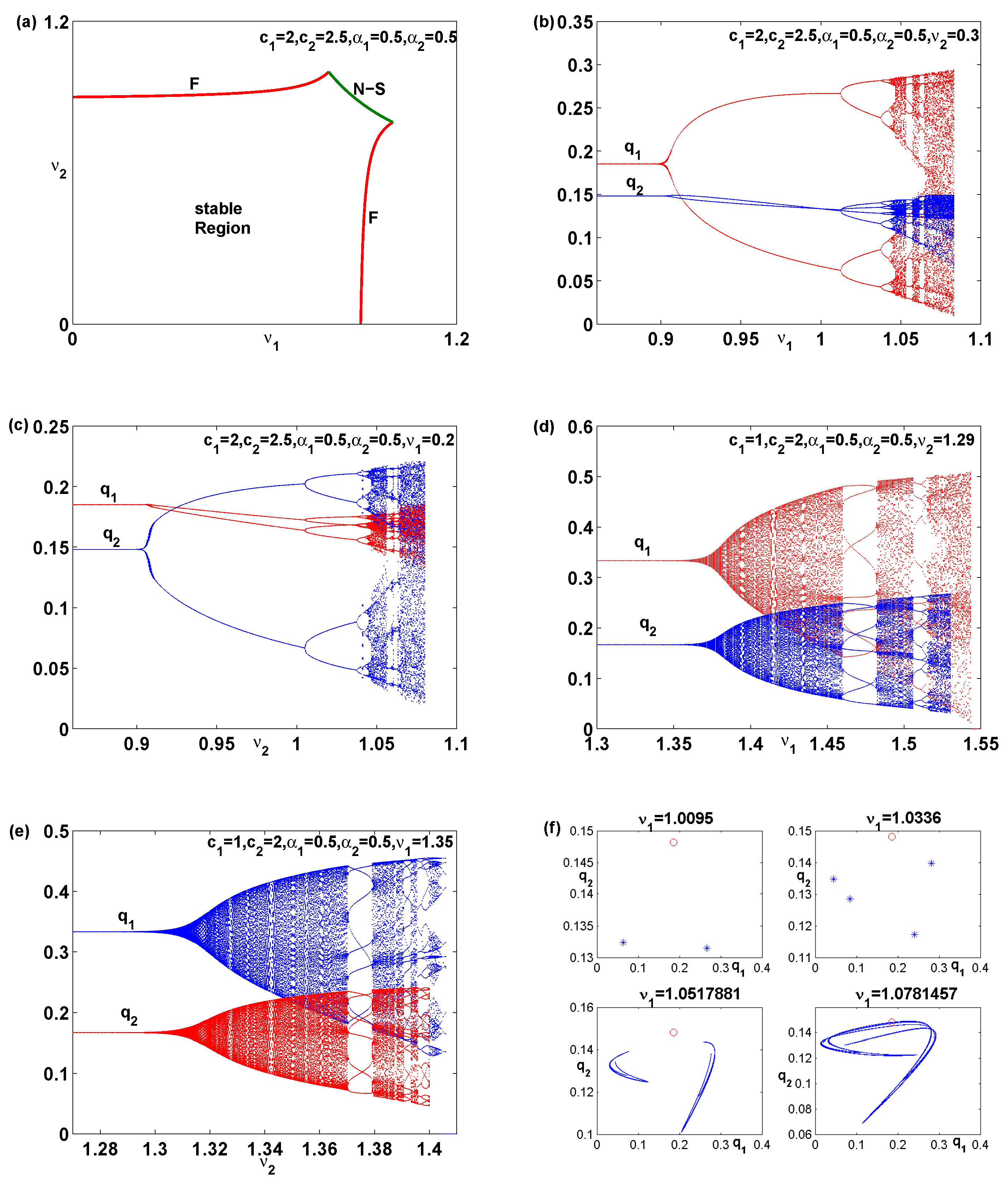
Figure 1. (a) The region of stability of Nash and the two types of bifurcations diagram at c 1 = 2 , c 2 = 2.5 , α 1 = 0.5 and α 2 = 0.5 . One-dimensional flip bifurcation diagram at c 1 = 2 , c 2 = 2.5 , α 1 = 0.5 , α 2 = 0.5 on varying (b) ν 1 and ν 2 = 0.3 . (c) ν 2 and ν 1 = 0.2 . One-dimensional Neimark–Sacker bifurcation diagram at c 1 = 1 , c 2 = 2 , α 1 = 0.5 , α 2 = 0.5 on varying (d) ν 2 and ν 1 = 1.35 . (e) ν 2 and ν 1 = 1.35 . (f) The phase plane of some periodic cycles and chaotic attractors at different values of ν 1 and c 1 = 2 , c 2 = 2.5 , α 1 = 0.5 , α 2 = 0.5 .
Symmetry 13 02235 g001
Figure 2. (a) The phase plane of closed invariant ring, periodic cycles and chaotic attractors at different values of ν 1 and c 1 = 1 , c 2 = 2 , α 1 = 0.5 , α 2 = 0.5 . The basin of attraction at c 1 = 2 , c 2 = 2.5 , α 1 = 0.5 , α 2 = 0.5 for (b) Period-2 cycle and ν 1 = 1.0095 and ν 2 = 0.3 . (c) Period-4 cycle and ν 1 = 1.0336 and ν 2 = 0.3 . (d) Two-bands chaotic attractor and ν 1 = 1.0517881 and ν 2 = 0.3 . (e) One chaotic attractor and ν 1 = 1.0781457 and ν 2 = 0.3 . (f) The basin of attraction of closed invariant ring at c 1 = 1 , c 2 = 2 , α 1 = 0.5 , α 2 = 0.5 , ν 1 = 1.4568456 and ν 2 = 1.29 .
Symmetry 13 02235 g002
Figure 3. The basin of attraction at c 1 = 1 , c 2 = 2 , α 1 = 0.5 , α 2 = 0.5 and ν 2 = 1.29 for (a) Period-8 cycle and ν 1 = 1.4725503 . (b) One chaotic attractor and ν 1 = 1.5208725 . (c) One chaotic attractor and ν 1 = 1.5408054 . (d) The main and secondary lobes for the chaotic attractor given in (c).
Symmetry 13 02235 g003
Figure 4. (a) The attractive basin for Nash point and ω 1 1 at the parameters values, c 1 = 1 , c 2 = 2 , α 1 = 0.5 , α 2 = 0.5 , ν 1 = 1.49 and ν 2 = 0.3 . (b) The preimage point of origin and both ω 1 1 and ω 2 1 for the attractive basin for the chaotic attractor given in Figure 3d.
Symmetry 13 02235 g004
Publisher’s Note: MDPI stays neutral with regard to jurisdictional claims in published maps and institutional affiliations.