Stochastic Comparisons of Lifetimes of Series and Parallel Systems with Dependent Heterogeneous MOTL-G Components under Random Shocks

Abstract

To measure the magnitude among random variables, we can apply a partial order connection defined on a distribution class, which contains the symmetry. In this paper, based on majorization order and symmetry or asymmetry functions, we carry out stochastic comparisons of lifetimes of two series (parallel) systems with dependent or independent heterogeneous Marshall–Olkin Topp Leone G (MOTL-G) components under random shocks. Further, the effect of heterogeneity of the shape parameters of MOTL-G components and surviving probabilities from random shocks on the reliability of series and parallel systems in the sense of the usual stochastic and hazard rate orderings is investigated. First, we establish the usual stochastic and hazard rate orderings for the lifetimes of series and parallel systems when components are statistically dependent. Second, we also adopt the usual stochastic ordering to compare the lifetimes of the parallel systems under the assumption that components are statistically independent. The theoretical findings show that the weaker heterogeneity of shape parameters in terms of the weak majorization order results in the larger reliability of series and parallel systems and indicate that the more heterogeneity among the transformations of surviving probabilities from random shocks according to the weak majorization order leads to larger lifetimes of the parallel system. Finally, several numerical examples are provided to illustrate the main results, and the reliability of series system is analyzed by the real-data and proposed methods.

1. Introduction

Order statistics plays a critical role in many research areas such as reliability theory, survival analysis, actuarial science, and auction theory. Let $X_{k:n}$ denote the k-th ordering statistics of random variables $X_1,X_2,\dots ,X_n$. In reliability theory, the lifetime of a (n − k + 1)-out-of-n system can be regarded as the k-th order statistic $X_{k:n}$. Particularly, the largest order statistics $X_{n:n}$ and the smallest order statistics $X_{1:n}$ correspond to the lifetimes of parallel and series systems, respectively. In auction theory, $X_{n:n}$ represents the winner’s price of the first-price English auction and $X_{1:n}$ represents the winner’s price in the first-price Dutch auction. In actuarial science, $X_{1:n}$ and $X_{n:n}$ correspond to the smallest and largest claim amounts in a portfolio of risks, respectively. Thus, the relevant topic of order statistics has attracted the attention of many researchers. In the past decades, stochastic comparisons of order statistics from heterogeneous samples have been discussed extensively in the literature. For example, one may refer to the works in [1,2,3,4,5,6,7,8] for details om different researches based on order statistics.

In the literature, there has been much to discuss on stochastic comparisons of lifetimes of series and parallel systems. For instance, Kochar and Torrado [9] established various ordering properties for parallel systems with independent scale components. Fang and Zhang [10] carried out stochastic comparisons of lifetimes of series systems with heterogeneous weibull components. Recently, Zhang et al. [11] compared the usual stochastic and reversed hazard rate orderings of two parallel systems with heterogeneous independent gamma components. For more relevant stochastic comparisons of lifetimes of systems, one can refer to the works in [12,13,14]. In this vein, systems in reliability engineering applications, however, may often be subject to random shocks such as an external stressing environment, competing soft and sudden failures [15]. These shocks cannot be neglected when considering the effects on the system’s lifetimes. Therefore, a more flexible model for series and parallel systems should consider the influence of random shocks on the system’s lifetime.

Consider a series or parallel system consisting of n independent or dependent components in working conditions. Each component of these systems suffering from random shocks can result in component failure. Suppose the random variable $X_i$ represents the lifetime of the i-th component in the series or parallel systems which may accept a random shock $I_{p_i}$ instantaneously. Furthermore, suppose that $I_{p_i}$ denotes independent Bernoulli random variables, independent of $X_i\prime s$, with $E\left(I_{p_i}\right)=p_i$, $i=1,2,\dots ,n$. When $I_{p_i}=1$, this random shock may not impact the i-th component with probability $p_i$, where $p_i$ means that the i-th component surviving probabilities subject to random shocks, while when $I_{p_i}=0$, this random shock will impact the i-th component with $1-p_i$ and result in its failure. Then, the components’ lifetimes can be considered as $I_{p_1}{X}_1,I_{p_2}{X}_2,\dots ,I_{p_n}{X}_n$ after a system consisting of n components suffering from random shocks. Thus, $Y_{1:n}$ = min$(Y_1,Y_2,\dots ,Y_n)$ and $Y_{n:n}$ = max$(Y_1,Y_2,\dots ,Y_n)$ correspond to the lifetimes of series and parallel systems subject to random shocks, respectively. One interesting topic is to investigate the influences of heterogeneity of components with the different lifetime distributions and random shocks on the lifetimes of series and parallel systems. For example, Kundu and Chowdhury [16] studied the effect of the heterogeneity of the frailty parameter of Kumaraswamy-G (Kw-G) components and surviving probabilities from random shocks on parallel systems with independent heterogeneous components by means of the row weakly majorization order. Kundu et al. [17] investigated the usual stochastic and hazard rate orderings when the vector of Gompertz–Makeham (GM) component parameters and vector of surviving probabilities were utilized in terms of the weak majorization order. Fang and Balakrishnan [18] discussed the effect heterogeneity of the vector of component parameters and vector of surviving probabilities on a series system with independent generalized Birnbaum–Saunders (GBS) component-associated random shocks. Zhang et al. [19] carried out stochastic comparisons between two fail-safe systems with independent components subject to random shocks in the sense of the usual stochastic, hazard rate, and likelihood ratio orderings. Das et al. [20] focused on the heterogeneity among the parameters of exponential location-scale components and surviving probabilities according to the multivariate chain majorization orders. For more details, one may refer to the works in [21,22,23,24,25,26,27]. All of the results mentioned above rely on the assumption that the lifetimes of the components are statistically independent. However, in practical reliability engineering, the lifetime of components may be statistically interdependent as all components of a system usually function in a common environment. In this regard, Li and Li [28] carried out stochastic comparisons between two series (parallel) systems equipped with starting devices regarding the hazard rate and the dispersive and usual stochastic orderings when the components are Gumbel–Hougaard–Copula-dependent. Panja et al. [29] investigated the usual stochastic and hazard rate orderings on series and parallel systems with dependent and heterogeneous components. For more relevant research the reliability of systems with dependent components, one can refer to the works in [30,31,32,33].

Based on the Marshall–Olkin Generalized (MOG) (see in [34]) and the Topp–Leone Generalized (TLG) (see in [35]) families, Khaleel et al. [36] introduced a new class of distributions called the Marshall–Olkin Topp Leone G (MOTL-G) family of distributions. The MOTL-G family of distributions are more flexible than the existing distributions including the gamma, exponential, Weibull, and log-normal, and increase the modeling ability of their baseline distributions in describing real-life events. More specially, each of the MOTL-G distributions can be obtained by a specified baseline distributed function G, for example, the MOTL-exponential (MOTL-E) distribution, the MOTL-Weibull (MOTL-We) distribution, and the MOTL-Lomax (MOTL-Lo) distribution. For more applications of the distribution, one may refer to Khaleel et al. [36]. A random variable X is said to follow the MOTL-G family, written as $X\sim MOTL-G(x;\alpha ,\beta ,\xi )$, if its distribution function is represented as

$$\begin{array}{c}\hfill \begin{array}{c}\hfill F_{\mathrm{MOTL}-\mathrm{G}}(x;\alpha ,\beta ,\xi )=\frac{{[1-{\left(1-G(x,\xi )\right)}^2]}^{\beta }}{\alpha +\overline{\alpha }{[1-{(1-G(x,\xi ))}^2]}^{\beta }},x\ge 0,\overline{\alpha }=1-\alpha ,\end{array}\end{array}$$

(1)

where $\alpha >0$ and $\beta >0$ are extra shape parameters, and x represents an independent variable of the function. In reliability engineering, x represents the realization value or age of the random life a component, and $G(x,\xi )$ is the baseline distributed function, which is dependent on parameter vector $\xi$. In particular, when $\alpha =1,$ the MOTL-G family reduces to the Topp Leone G family. Due to the complexity of the distribution, in this manuscript we study the special case of $G(x,\xi )=G\left(x\right)$. The MOTL-G distribution is a flexible probability model, which makes it very helpful for the modeling of real-life data and to characterize component lifetimes. However, to the best of our knowledge, no research work has been done on stochastic comparisons of the lifetimes of series and parallel systems with dependent heterogeneous MOTL-G components subject to random shocks. In this work, we will establish sufficient conditions to stochastically compare two series (parallel) systems with dependent heterogeneous MOTL-G components bearing independent random shocks.

Symmetry is usually used to refer to an object that is invariant under some transformations. In fact, we find that some reliability functions are exactly permutation-invariant with respect to parameters, that is, the reliability functions are symmetric. For the ordering of majorization, the theorem of Muirhead [37] gave some methods to prove the order-preserving functions, which are useful to construct variety inequalities about partial ordering. For a comprehensive study of the functions preserving the ordering of majorization, one can refer to Marshall et al. [38]. The reliability of the system refers to the probability that the components will work normally under the specified conditions (such as temperature, humidity, shock and electric field, etc.) and the specified time, the lifetime of the system refers to the duration time of the system components normally work under certain operating conditions, it can be seen from the definitions that the reliability of the system is related to time and is therefore related to the systems lifetime, and non-negative random variables are used to express the duration time of certain state in nature, human society, or technological progress [39]. Suppose that T represents the lifetimes of the system under specified conditions, $t_0$ is a given positive number, and $P(T>t_0)$ represents the reliability of the system. Therefore, the reliability of a system is characterized by the survival functions of system. This means that larger system lifetime leads to higher system reliability, and smaller system lifetime results in lower system reliability. The novelty of this paper is that it makes use of the MOTL-G distributions to describe component lifetime and considers the dependence between components and the effect random shocks on the reliability of system. The purposes of this research are listed below.

(1) The effect of the heterogeneity of the shape parameters of MOTL-G components and surviving probabilities from random shocks on the reliability of series and parallel systems with dependent heterogeneous components is investigated.

(2) The influence of the heterogeneity of the shape parameters of MOTL-G components and surviving probabilities from random shocks on the reliability of parallel system with independent heterogeneous component is studied.

The main task of this paper is based on stochastic order, majorization order, Schur-convex or Schur-concave, and the symmetric or asymmetric nature of functions.

(1) We will carry out the stochastic comparisons of the lifetimes of series and parallel systems from two sets of dependent heterogeneous MOTL-G components under random shocks.

(2) We will also compare the lifetimes of parallel systems with independent heterogeneous MOTL-G components subject to random shocks.

The rest of this paper is organized as follows. In Section 2, we recall some fundamental notations of the stochastic order, majorization order, and Archimedean copula, and present some lemmas. Section 3 deals with the stochastic comparison of series and parallel systems with dependent or independent components under random shocks. The result is adopted to assess the reliability of series systems in Section 4. In Section 5, we compare the results of the experiment and the obtained theoretical data. Finally, some innovations, practical conclusions and future topics are outlined in Section 6.

2. Preliminaries

Throughout the paper, we use the notation “$a\stackrel{sgn}{=}b$” to show that a and b have the same sign and $h^{-1}$ denotes the inverse of monotonic function h. The term “increasing” represents “non-decreasing” and “decreasing” means “non-increasing”. It is also assumed that random variables mentioned in this paper are non-negative and absolutely continuous.

Before proceeding to the main results, we first recall some concepts of stochastic orders, Majorization orders, and copula, which will be used in the sequel.

2.1. Stochastic Order

Suppose that X is a random variable having the cumulative distribution $F_X$, density function $f_X$, survival function ${\overline{F}}_X$, hazard rate function $r_X$, and reversed hazard rate function ${\tilde{r}}_X$.

Definition 1.

For two random variables X and Y, X is said to be smaller than Y in the

 (i) 

usual stochastic order (denoted by $X{\le }_{st}Y$) if ${\overline{F}}_X\left(x\right)\le {\overline{F}}_Y\left(x\right)$ for all $x\in (-\infty ,\infty )$;

 (ii) 

hazard rate order (denoted by $X{\le }_{hr}Y$) if ${\overline{F}}_Y\left(x\right)/{\overline{F}}_X\left(x\right)$ is increasing in $x\in (-\infty ,\infty )$ or, equivalently, $r_X\left(x\right)\ge r_Y\left(x\right)$;

 (iii) 

reversed hazard rate order (denoted by $X{\le }_{rh}Y$) if $F_Y\left(x\right)/F_X\left(x\right)$ is increasing in $x\in (-\infty ,\infty )$ or, equivalently, ${\tilde{r}}_X\left(x\right)\le {\tilde{r}}_Y\left(x\right).$

It is well known that the hazard rate order or the reversed hazard rate order implies the usual stochastic order, but the reverse is not true. For more detailed discussions and applications of stochastic orders, please refer to Shaked and Shanthikumar [40].

2.2. Majorization Order

Let $x_{1:n}\le x_{2:n}\le \dots \le x_{n:n}$ and $y_{1:n}\le y_{2:n}\le \dots \le y_{n:n}$ be the increasing arrangement of the components of vector $\mathit{x}=(x_1,x_2,\dots ,x_n)$ and $\mathit{y}=(y_1,y_2,\dots ,y_n)$, respectively.

Definition 2.

For two real vectors $\mathit{x}=(x_1,x_2,\dots ,x_n)$ and $\mathit{y}=(y_1,y_2,\dots ,y_n)$, $\mathit{x}$ is said to

 (i) 

majorize $\mathit{y}$ (denoted as $\mathit{x}\stackrel{m}{⪰}\mathit{y}$), if ${\displaystyle \sum _{i=1}^j}{x}_{i:n}\le {\displaystyle \sum _{i=1}^j}{y}_{i:n},$ for $j=1,2,\dots ,n-1$, and ${\displaystyle \sum _{i=1}^n}{x}_{i:n}={\displaystyle \sum _{i=1}^n}{y}_{i:n}$;

 (ii) 

weakly supermajorize $\mathit{y}$ (denoted by $\mathit{x}\stackrel{w}{⪰}\mathit{y}$), if ${\displaystyle \sum _{i=1}^j}{x}_{i:n}\le {\displaystyle \sum _{i=1}^j}{y}_{i:n}$, for $j=1,2,\dots ,n$;

 (iii) 

weakly submajorize $\mathit{y}$ (denoted by $\mathit{x}{⪰}_w\mathit{y}$), if ${\displaystyle \sum _{j=i}^n}{x}_{j:n}\ge {\displaystyle \sum _{j=i}^n}{y}_{j:n},$ for $i=1,2,\dots ,n$.

Definition 3.

A real-valued function ϕ defined on a set $\mathcal{A}\in {\mathbb{R}}^n$ is said to be Schur-convex (Schur-concave) on $\mathcal{A}$ if $\mathit{x}\stackrel{m}{⪯}\mathit{y}$ implies $\varphi \left(\mathit{x}\right)\le (\ge )\varphi \left(\mathit{y}\right)$ on $\mathcal{A}$.

Definition 4.

Let $A={\left(a_{ij}\right)}_{m\times n}$ and $B={\left(b_{ij}\right)}_{m\times n}$ be two $m\times n$ matrices with rows ${\mathbf{a}}_i:=(a_{i1},a_{i2},\dots ,a_{in})$ and ${\mathbf{b}}_i:=(b_{i1},b_{i2},\dots ,b_{in})$ for $i=1,2,\dots ,m$, respectively. A is said to be larger than the matrix B in the

 (i) 

row majorization (denoted as $A{>}^{row}B$), if ${\mathbf{a}}_i\stackrel{m}{⪰}{\mathbf{b}}_i$ for $i=1,2,\dots ,m$;

 (ii) 

row weakly majorization (denoted as $A{>}^{w}B$), if ${\mathbf{a}}_i\stackrel{w}{⪰}{\mathbf{b}}_i$ for $i=1,2,\dots ,m$.

Clearly, it is known that the majorization order implies that the weak supermajorization order or the weak submajorization order. For more details discussion and their applications, one may refer to Marshall et al. [38].

2.3. Archimedean Copula

Definition 5.

For a decreasing and continuous function $\psi :[0,+\infty ]\to [0,1]$ such that $\psi \left(0\right)=1$ and $\psi (+\infty )=0,$ let $\varphi ={\psi }^{-1}$ be the pseudo-inverse. Then,

$$C_{\psi }(u_1,...,u_n)=\psi (\varphi \left(u_1\right)+...+\varphi \left(u_n\right)),forall{u}_i\in [0,1],i=1,2,\dots ,n,$$

is said to be an Archimedean copula with the generator $\psi ,$ if ${(-1)}^k{\psi }^k\left(x\right)\ge 0,\mathrm{for}k=0,1,\dots ,n-2$ and ${(-1)}^{n-2}{\psi }^{n-2}\left(x\right)$ is decreasing and convex.

For more on Archimedean copula, readers may refer to Nelsen [41].

2.4. Some Useful Lemmas

For convenience, from now on, we denote

${\mathcal{D}}_{+}=\left\{\left(x_1,x_2,\dots ,x_n\right):x_1\ge x_2\ge \dots \ge x_n>0\right\},$

${\mathcal{E}}_{+}=\left\{\left(x_1,x_2,\dots ,x_n\right):0<x_1\le x_2\le \dots \le x_n\right\},$

$${\mathcal{U}}_n=\left\{(\mathit{x},\mathit{y})=\left(\begin{array}{cccc}{x}_1& x_2& \dots & x_n\\ y_1& y_2& \dots & y_n\end{array}\right):(x_i-x_j)(y_i-y_j)\ge 0,i,j=1,2,\dots ,n\right\},$$

and

$${\mathcal{V}}_n=\left\{(\mathit{x},\mathit{y})=\left(\begin{array}{cccc}{x}_1& x_2& \dots & x_n\\ y_1& y_2& \dots & y_n\end{array}\right):(x_i-x_j)(y_i-y_j)\le 0,i,j=1,2,\dots ,n\right\}.$$

Before proceeding to main results, we first introduce some lemmas utilized in the sequel. The proofs of Lemmas 1 and 2 are simple and therefore are omitted.

Lemma 1.

The function

$$\eta (x,y,z)=\frac{{(1-{(1-z)}^2)}^{y}log(1-{(1-z)}^2)}{(x+(1-x){(1-{(1-z)}^2)}^y)(1-{(1-{(1-z)}^2)}^y)},$$

where $(x,y,z)\in (0,+\infty )\times (0,+\infty )\times [0,1],$ is increasing in x and y.

Lemma 2.

Let the function $\zeta :(0,+\infty )\times (0,+\infty )\times [0,1]\to [0,1]$ be defined as

$$\zeta (x,y,z)=\frac{x(1-{(1-{(1-z)}^2)}^y)}{x+(1-x){(1-{(1-z)}^2)}^y}.$$

Then,

 (i) 

$\zeta (x,y,z)$ is increasing in $x\in (0,+\infty )$ and $y\in (0,+\infty )$;

 (ii) 

$\zeta (x,y,z)$ is decreasing in $z\in [0,1]$.

 Lemma 3

(Marshall et al. [38]. Theorem 3.A.4). Suppose $J\subset \mathbb{R}$ be an open interval and $\varphi \left(\mathit{y}\right):J^n\to \mathbb{R}$ is continuously differentiable. Then, $\varphi \left(\mathit{y}\right)$ is Schur-convex (Schur-concave) on $J^n$, if and only if

 (i) 

$\varphi \left(\mathit{y}\right)$ is symmetric on $J^n$,

 (ii) 

for all $i\ne j$ and all $\mathit{y}\in J^n$,

$$(y_i-y_j)\left(\frac{\partial \varphi \left(\mathit{y}\right)}{\partial y_i}-\frac{\partial \varphi \left(\mathit{y}\right)}{\partial y_j}\right)\ge (\le )0.$$

In the case of asymmetrical multivariate functions, Lemmas 4 and 5 provide a necessary and sufficient condition for preserving the majorization order.

Lemma 4

(Kundu et al. [16]. Lemma 2.1). Let $\phi :{\mathcal{D}}_{+}\to \mathfrak{R}$ be a function, continuously differentiable on the interior of ${\mathcal{D}}_{+}$. Then, for $\mathit{x},\mathit{y}\in {\mathcal{D}}_{+}$,

$$\mathit{x}\stackrel{\mathrm{m}}{⪰}\mathit{y}\mathrm{implies}\phi \left(\mathit{x}\right)\ge (\mathrm{resp}.\le )\phi \left(\mathit{y}\right)$$

if, and only if

$${\phi }_{\left(k\right)}\left(\mathit{z}\right)\mathrm{is}decreasing(resp.increasing)ink=1,2,\dots ,n$$

where ${\phi }_{\left(k\right)}\left(\mathit{z}\right)=\partial \phi \left(\mathit{z}\right)/\partial z_k$ denotes the partial derivative of φ with respect to its $kth$ argument.

Lemma 5

(Kundu et al. [16]. Lemma 2.2). Let $\phi :{\mathcal{E}}_{+}\to \mathfrak{R}$ be a function, continuously differentiable on the interior of ${\mathcal{E}}_{+}$. Then, for $\mathit{x},\mathit{y}\in {\mathcal{E}}_{+}$,

$$\mathit{x}\stackrel{\mathrm{m}}{⪰}\mathit{y}implies\phi \left(\mathit{x}\right)\ge (resp.\le )\phi \left(\mathit{y}\right)$$

if and only if

$${\phi }_{\left(k\right)}\left(\mathit{z}\right)\mathrm{is}increasing(resp.decreasing)ink=1,2,\dots ,n$$

where ${\phi }_{\left(k\right)}\left(\mathit{z}\right)=\partial \phi \left(\mathit{z}\right)/\partial z_k$ denotes the partial derivative of φ with respect to its $kth$ argument.

Lemma 6

(Kundu et al. [16]. Lemma 2.3). A real valued function ψ on $\mathcal{A}\subseteq {\mathbb{R}}^n$, satisfies

 (i) 

$\mathit{x}{⪰}_{\mathrm{w}}\mathit{y}$ implies $\psi \left(\mathit{x}\right)\ge (resp.\le )\psi \left(\mathit{y}\right)$ if and only if ψ is increasing (resp. decreasing) Schur-convex (resp. Schur-concave) on $\mathcal{A}$;

 (ii) 

$\mathit{x}\stackrel{\mathrm{w}}{⪰}\mathit{y}$ implies $\psi \left(\mathit{x}\right)\ge (resp.\le )\psi \left(\mathit{y}\right)$ if and only if ψ is decreasing (resp. increasing) Schur-convex (resp. Schur-concave) on $\mathcal{A}$.

Lemma 7

(Fang et al. [42] Lemma 3.8). For two n-dimensional Archimedean copulas $C_{{\psi }_1}$ and $C_{{\psi }_2}$, if ${\varphi }_2\circ {\psi }_1$ is super-additive, then $C_{{\psi }_1}\left(\mathit{u}\right)\le C_{{\psi }_2}\left(\mathit{u}\right)$ for all $\mathit{u}\in {[0,1]}^n$.

3. Main Results

In this section, we establish comparison results between two series (parallel) systems with dependent or independent heterogeneous MOTL-G distributed components under the different surviving probabilities subject to random shocks in the sense of stochastic orderings. Assume that $Z_1$ and $Z_2$ are two random variables with continuous distribution functions $G_1(·)$ and $G_2(·)$, respectively. Further, let $\mathit{X}=(X_1,\dots ,X_n)$ be a set of dependent MOTL-G-distributed random vectors with $X_i\sim MOTL-G({\alpha }_i,{\beta }_i,G_1\left(x\right))$, $i=1,2,\dots ,n$, and an Archimedean copula having generator ${\psi }_1$$({\varphi }_1={\psi }_1^{-1})$. Similarly, let ${\mathit{X}}^{*}=(X_1^{*},\dots ,X_n^{*})$ be a set of dependent MOTL-G-distributed random vectors with $X_i^{*}\sim MOTL-G({\gamma }_i,{\delta }_i,G_2\left(x\right))$, $i=1,2,\dots ,n$, and an Archimedean copula having generator ${\psi }_2$$({\varphi }_2={\psi }_2^{-1})$. Also suppose $I_{p_1},\dots ,I_{p_n}$$(I_{p_i^{*}},\dots ,I_{p_i^{*}})$ be a set of independent Bernoulli random variables with $E\left(I_{p_i}\right)=p_i$ ($E\left(I_{p_i^{*}}\right)=p_i^{*}$), independent of $X_i\prime s(X_i^{*}\prime s)$, $i=1,2,\dots ,n$. Denote $Y_i=X_i{I}_{p_i}$ and $Y_i^{*}=X_i^{*}{I}_{p_i}^{*}$.

3.1. Heterogeneous Dependent Case

In this subsection, we assume that series and parallel systems are made up of dependent heterogeneous components, and the components of system dependence structure are captured by Archimedean copula.

3.1.1. Comparison of Two Series Systems

In this subsection, we investigate the effect of heterogeneity among shape parameters and surviving probabilities from random shocks on the reliabilities of two series systems with dependent heterogeneous MOTL-G distributed components in the sense of usual stochastic and hazard rate orderings. Suppose that ${\overline{F}}_{X_{1:n}}\left(x\right)$ and ${\overline{F}}_{X_{1:n}^{*}}\left(x\right)$ are the reliability functions of $X_{1:n}$ and $X_{1:n}^{*}$. Then, from Equation (1), the survival functions of $X_{1:n}$ and $X_{1:n}^{*}$ are given by

$$\begin{array}{c}\hfill \begin{array}{cc}\hfill {\overline{F}}_{X_{1:n}}\left(x\right)& ={\psi }_1\left(\sum _{i=1}^n{\varphi }_1\left(\frac{{\alpha }_i\left(1-{\left(1-{\left(1-G_1\left(x\right)\right)}^2\right)}^{{\beta }_i}\right)}{{\alpha }_i+{\overline{\alpha }}_i{\left(1-{\left(1-G_1\left(x\right)\right)}^2\right)}^{{\beta }_i}}\right)\right)\hfill \\ & ={\psi }_1\left(\sum _{i=1}^n{\varphi }_1\left(\zeta ({\alpha }_i,{\beta }_i,G_1\left(x\right))\right)\right)\hfill \end{array}\end{array}$$

(2)

and

$$\begin{array}{c}\hfill \begin{array}{cc}\hfill {\overline{F}}_{X_{1:n}^{*}}\left(x\right)& ={\psi }_2\left(\sum _{i=1}^n{\varphi }_2\left(\frac{{\gamma }_i\left(1-{\left(1-{\left(1-G_2\left(x\right)\right)}^2\right)}^{{\delta }_i}\right)}{{\gamma }_i+{\overline{\gamma }}_i{\left(1-{\left(1-G_2\left(x\right)\right)}^2\right)}^{{\delta }_i}}\right)\right)\hfill \\ & ={\psi }_2\left(\sum _{i=1}^n{\varphi }_2\left(\zeta ({\gamma }_i,{\delta }_i,G_2\left(x\right))\right)\right),\hfill \end{array}\end{array}$$

(3)

respectively, and the survival function of $Y_{1:n}$ is given by

$$\begin{array}{c}\hfill \begin{array}{cc}\hfill {\overline{F}}_{Y_{1:n}}\left(x\right)=& P(Y_1>x,Y_2>x,\dots ,Y_n>x)\hfill \\ \hfill =& P(X_1{I}_{p_1}>x,X_2{I}_{p_2}>x,\dots ,X_n{I}_{p_n}>x|I_{p_i}=1,1\le i\le n)P(I_{p_i}=1,1\le i\le n)\hfill \\ \hfill =& P(X_1>x,X_2>x,\dots ,X_n>x)P(I_{p_1}=1,I_{p_2}=1,\dots ,I_{p_n}=1)\hfill \\ \hfill =& \prod _{i=1}^n{p}_i{\overline{F}}_{X_{1:n}}\left(x\right).\hfill \end{array}\end{array}$$

(4)

Similarly, $Y_{1:n}^{*}\left(x\right)$ has survival function

$${\overline{F}}_{Y_{1:n}^{*}}\left(x\right)=\prod _{i=1}^n{p}_i^{*}{\overline{F}}_{X_{1:n}^{*}}\left(x\right).$$

Note that ${\overline{F}}_{Y_{1:n}}\left(0\right)=\prod _{i=1}^n{p}_i$ and ${\overline{F}}_{Y_{1:n}^{*}}\left(0\right)=\prod _{i=1}^n{p}_i^{*}$.

The following Theorems 1 and 2 investigate the effect of heterogeneity of shape parameters on the reliabilities of series systems in sense of the usual stochastic order, respectively.

Theorem 1.

Suppose $X_1,\dots ,X_n$$(X_1^{*},\dots ,X_n^{*})$ be a set of dependent MOTL-G random variables having Archimedean copula with generator ${\psi }_1$$\left({\psi }_2\right)$ such that $X_i\sim MOTL-G({\alpha }_i,{\beta }_i,G_1\left(x\right))$$(X_i^{*}\sim MOTL-G({\alpha }_i,{\delta }_i,G_2\left(x\right)))$, $i=1,2,\dots ,n$. Further assume $I_{p_1},\dots ,$$I_{p_n}$$(I_{p_1^{*}},\dots ,I_{p_n^{*}})$ be a set of independent Bernoulli random variables with $E\left(I_{p_i}\right)=p_i$$(E\left(I_{p_i^{*}}\right)=p_i^{*})$, independent of $X_i\prime s(X_i^{*}\prime s)$, $i=1,2,\dots ,n$. If

(i)$(\alpha ,\beta )\in {\mathcal{U}}_n$and$(\alpha ,\delta )\in {\mathcal{U}}_n$,

(ii)$Z_1{\le }_{st}{Z}_2$,

(iii)$\prod _{i=1}^n{p}_i\le \prod _{i=1}^n{p}_i^{*}$ and

(iv)${\varphi }_2\circ {\psi }_1$is super-additive and${\psi }_1$ or ${\psi }_2$ is log-convex, then

$$\left({\beta }_1,{\beta }_2,\dots ,{\beta }_n\right)\stackrel{w}{⪰}\left({\delta }_1,{\delta }_2,\dots ,{\delta }_n\right)⟹Y_{1:n}{\le }_{st}{Y}_{1:n}^{*}.$$

Proof of Theorem 1. 

From (4), the survival function of $Y_{1:n}$ can be written as

$$\begin{array}{c}\hfill \begin{array}{c}\hfill {\overline{F}}_{Y_{1:n}}\left(x\right)=\prod _{i=1}^n{p}_i{\overline{F}}_{X_{1:n}}\left(x\right)=\prod _{i=1}^n{p}_i{\psi }_1\left(\sum _{i=1}^n{\varphi }_1\left(\zeta ({\alpha }_i,{\beta }_i,G_1\left(x\right))\right)\right).\end{array}\end{array}$$

Similarly, the survival function of $Y_{1:n}^{*}$ is

$$\begin{array}{c}\hfill \begin{array}{c}\hfill {\overline{F}}_{Y_{1:n}^{*}}\left(x\right)=\prod _{i=1}^n{p}_i^{*}{\overline{F}}_{X_{1:n}^{*}}\left(x\right)=\prod _{i=1}^n{p}_i^{*}{\psi }_2\left(\sum _{i=1}^n{\varphi }_2\left(\zeta ({\alpha }_i,{\delta }_i,G_2\left(x\right))\right)\right).\end{array}\end{array}$$

To prove the required result, according to the condition of ${\prod }_{i=1}^n{p}_i\le {\prod }_{i=1}^n{p}_i^{*}$, it is enough to show that ${\overline{F}}_{X_{1:n}}\left(x\right)\le {\overline{F}}_{X_{1:n}^{*}}\left(x\right)$. Without loss of generality, we assume that ${\psi }_1$ is log-convex, $\mathbf{\alpha }\in {\mathcal{E}}_{+}$, and $\mathbf{\beta }\in {\mathcal{E}}_{+}$. The super-additively of ${\varphi }_2\circ {\psi }_1$ implies that

$$\begin{array}{c}\hfill \begin{array}{c}\hfill {\psi }_1\left(\sum _{i=1}^n{\varphi }_1\left(\zeta ({\alpha }_i,{\delta }_i,G_2\left(x\right))\right)\right)\le {\psi }_2\left(\sum _{i=1}^n{\varphi }_2\left(\zeta ({\alpha }_i,{\delta }_i,G_2\left(x\right))\right)\right).\end{array}\end{array}$$

(5)

According to Lemma 2 and $Z_1{\le }_{st}{Z}_2$, we have $\zeta ({\alpha }_i,{\delta }_i,G_1\left(x\right))\le \zeta ({\alpha }_i,{\delta }_i,G_2\left(x\right))$. Again, the decreasing property of ${\varphi }_1$ and ${\psi }_1$ implies that

$$\begin{array}{c}\hfill \begin{array}{c}\hfill {\psi }_1\left(\sum _{i=1}^n{\varphi }_1\left(\zeta ({\alpha }_i,{\delta }_i,G_1\left(x\right))\right)\right)\le {\psi }_1\left(\sum _{i=1}^n{\varphi }_1\left(\zeta ({\alpha }_i,{\delta }_i,G_2\left(x\right))\right)\right).\end{array}\end{array}$$

(6)

Combining (5) and (6), we conclude

$${\psi }_1\left(\sum _{i=1}^n{\varphi }_1\left(\zeta ({\alpha }_i,{\delta }_i,G_1\left(x\right))\right)\right)\le {\psi }_2\left(\sum _{i=1}^n{\varphi }_2\left(\zeta ({\alpha }_i,{\delta }_i,G_2\left(x\right))\right)\right).$$

Therefore, to prove that

$${\psi }_1\left(\sum _{i=1}^n{\varphi }_1\left(\zeta ({\alpha }_i,{\beta }_i,G_1\left(x\right))\right)\right)\le {\psi }_2\left(\sum _{i=1}^n{\varphi }_2\left(\zeta ({\alpha }_i,{\delta }_i,G_2\left(x\right))\right)\right),$$

it is sufficient to show that

$${\psi }_1\left(\sum _{i=1}^n{\varphi }_1\left(\zeta ({\alpha }_i,{\beta }_i,G_1\left(x\right))\right)\right)\le {\psi }_1\left(\sum _{i=1}^n{\varphi }_1\left(\zeta ({\alpha }_i,{\delta }_i,G_1\left(x\right))\right)\right).$$

Clearly, for ${\alpha }_1={\alpha }_2=\dots ={\alpha }_n$, ${\psi }_1\left(\sum _{i=1}^n{\varphi }_1\left(\zeta ({\alpha }_i,{\beta }_i,G_1\left(x\right))\right)\right)$ with respect to $\mathbf{\beta }$ is symmetric. When ${\alpha }_1\ne {\alpha }_2\ne \dots \ne {\alpha }_n$, ${\psi }_1\left(\sum _{i=1}^n{\varphi }_1\left(\zeta ({\alpha }_i,{\beta }_i,G_1\left(x\right))\right)\right)$ in $\mathbf{\beta }$ is asymmetric. By Lemma 6, we only need to show that ${\mathrm{\Psi }}_1(\mathbf{\alpha },\mathbf{\beta },{\psi }_1,G_1\left(x\right))={\psi }_1\left(\sum _{i=1}^n{\varphi }_1\left(\zeta ({\alpha }_i,{\beta }_i,G_1\left(x\right))\right)\right)$ is increasing and Schur-concave in $\mathbf{\beta }$. The partial derivative of ${\mathrm{\Psi }}_1(\mathbf{\alpha },\mathbf{\beta },{\psi }_1,G_1\left(x\right))$ with respect to ${\beta }_j$ is given by

$$\begin{array}{ccc}& & \frac{\partial {\mathrm{\Psi }}_1(\mathbf{\alpha },\mathbf{\beta },{\psi }_1,G_1\left(x\right))}{\partial {\beta }_j}\hfill \\ & =& -\eta ({\alpha }_j,{\beta }_j,G_1\left(x\right))\times \frac{{\psi }_1\left({\varphi }_1\left(\zeta ({\alpha }_j,{\beta }_j,G_1\left(x\right))\right)\right)}{{\psi }_1^{\prime }\left({\varphi }_1\left(\zeta ({\alpha }_j,{\beta }_j,G_1\left(x\right))\right)\right)}\times {\psi }_1^{\prime }\left(\sum _{i=1}^n{\varphi }_1\left(\zeta ({\alpha }_i,{\beta }_i,G_1\left(x\right))\right)\right)\hfill \\ & =& -\eta ({\alpha }_j,{\beta }_j,G_1\left(x\right))\times k({\alpha }_j,{\beta }_j,G_1\left(x\right))\times {\psi }_1^{\prime }\left(\sum _{i=1}^n{\varphi }_1\left(\zeta ({\alpha }_i,{\beta }_i,G_1\left(x\right))\right)\right),\hfill \end{array}$$

where $k({\alpha }_j,{\beta }_j,G_1\left(x\right))=\frac{{\psi }_1\left({\varphi }_1\left(\zeta ({\alpha }_j,{\beta }_j,G_1\left(x\right))\right)\right)}{{\psi }_1^{\prime }\left({\varphi }_1\left(\zeta ({\alpha }_j,{\beta }_j,G_1\left(x\right))\right)\right)}$, and $\eta$ and $\zeta$ are the functions defined in Lemmas 1 and 2, respectively. As ${\psi }_1$ is n-monotone and $\eta (\alpha ,\beta ,G_1\left(x\right))$ is non-positive, we have ${\psi }_1^{\prime }\le 0$ and ${\mathrm{\Psi }}_1(\alpha ,\beta ,{\psi }_1,G\left(x\right))$ is increasing with respect to ${\beta }_j$ for any $x\ge 0$. Note that for $j=1,2,\dots ,n$, we have

$$\begin{array}{cc}\hfill \frac{\partial k({\alpha }_j,{\beta }_j,G_1\left(x\right))}{\partial {\beta }_j}=& \frac{\partial \zeta ({\alpha }_j,{\beta }_j,G_1\left(x\right))/\partial {\beta }_j}{{\left[{\psi }_1^{{}^{\prime }}\left({\varphi }_1\left(\zeta ({\alpha }_j,{\beta }_j,G_1\left(x\right))\right)\right)\right]}^3}\times \left\{{\left[{\psi }_1^{{}^{\prime }}\left({\varphi }_1\left(\zeta ({\alpha }_j,{\beta }_j,G_1\left(x\right))\right)\right)\right]}^2\right.\hfill \\ \hfill & \phantom{=}\left.-{\psi }_1^{{}^{\prime \prime }}\left({\varphi }_1\left(\zeta ({\alpha }_j,{\beta }_j,G_1\left(x\right))\right)\right){\psi }_1^{{}^{\prime }}\left({\varphi }_1\left(\zeta ({\alpha }_j,{\beta }_j,G_1\left(x\right))\right)\right)\right\}.\hfill \end{array}$$

In view of Lemma 2, the function $\zeta ({\alpha }_j,{\beta }_j,G_1\left(x\right))$ is increasing in ${\beta }_j$ for $j=1,2,\dots ,n$, and considering that ${\psi }_1$ is log-convex, we conclude that

$$\frac{{\partial }^{2}ln{\psi }_1\left(x\right)}{\partial x^2}=\frac{{\psi }_1^{{}^{\prime \prime }}\left(x\right){\psi }_1\left(x\right)-{\left({\psi }_1^{{}^{\prime }}\left(x\right)\right)}^2}{{\psi }_1^2\left(x\right)}\ge 0,$$

and

$$\frac{\partial \zeta ({\alpha }_j,{\beta }_j,G_1\left(x\right))}{\partial {\beta }_j}\ge 0.$$

Thus, $k({\alpha }_j,{\beta }_j,G_1\left(x\right))$ is non-positive and increasing in ${\beta }_j$, for $j=1,2,\dots ,n$. Similarly, we also obtain that $k({\alpha }_j,{\beta }_j,G_1\left(x\right))$ is non-positive and increasing in ${\alpha }_j$, for $j=1,2,\dots ,n$. On the other hand, by Lemma 1, it is easy to show that $\eta ({\alpha }_j,{\beta }_j,G_1\left(x\right))$ is non-positive and increasing in ${\beta }_j$ and ${\alpha }_j$. Therefore, $\eta ({\alpha }_j,{\beta }_j,G_1\left(x\right))k({\alpha }_j,{\beta }_j,G_1\left(x\right))$ is decreasing in ${\beta }_j$ and ${\alpha }_j$. Then, for any $i\ne j$, we have

$$\begin{array}{ccc}& & \left(\frac{\partial {\mathrm{\Psi }}_1(\alpha ,\beta ,{\psi }_1,G_1\left(x\right))}{\partial {\beta }_i}-\frac{\partial {\mathrm{\Psi }}_1(\alpha ,\beta ,{\psi }_1,G_2\left(x\right))}{\partial {\beta }_j}\right)\hfill \\ & =& -\left(\eta ({\alpha }_i,{\beta }_i,G_1\left(x\right))k({\alpha }_i,{\beta }_i,G_1\left(x\right))-\eta ({\alpha }_j,{\beta }_j,G_1\left(x\right))k({\alpha }_j,{\beta }_j,G_1\left(x\right))\right)\hfill \\ & & \times {\psi }_1^{\prime }\left(\sum _{i=1}^n{\varphi }_1\left(\zeta ({\alpha }_i,{\beta }_i,z)\right)\right)\ge 0.\hfill \end{array}$$

Thus, the Schur-concavity of ${\mathrm{\Psi }}_1(\alpha ,\beta ,{\psi }_1,G_1\left(x\right))$ follows immediately from Lemma 5. Note that $\beta \stackrel{\mathrm{w}}{⪰}\delta$, we obtain ${\psi }_1\left({\sum }_{i=1}^n{\varphi }_1\left(\zeta ({\alpha }_i,{\beta }_i,G_1\left(x\right))\right)\right)\le {\psi }_1\left({\sum }_{i=1}^n{\varphi }_1\left(\zeta ({\alpha }_i,{\delta }_i,G_1\left(x\right))\right)\right)$ by Lemma 6. The proof is completed. □

Remark 1.

When ${\displaystyle \prod _{i=1}^n}{p}_i={\displaystyle \prod _{i=1}^n}{p}_i^{*}$ and $\alpha =1$, the result of Theorem 1 is similar to Theorem 2 of Zhang and Yan [43] for fixed the parameter $\theta =1$. It should be mentioned that Zhang and Yan [43] only studied the effect of heterogeneity components on the reliability of the series and parallel systems, while ignoring the effect of random shocks on the reliability of system.

The following result can be proved by using a similar proof method with that of Theorem 1, which is omitted here for brevity.

Theorem 2.

Suppose $X_1,\dots ,X_n$$(X_1^{*},\dots ,X_n^{*})$ is a set of dependent MOTL-G random variables having Archimedean copula with generator ${\psi }_1$$\left({\psi }_2\right)$ such that $X_i\sim MOTL-G({\alpha }_i,{\beta }_i,G_1\left(x\right))$$(X_i^{*}\sim MOTL-G({\gamma }_i,{\beta }_i,G_2\left(x\right)))$, $i=1,2,\dots ,n$. Further, assume that $I_{p_1},\dots ,$$I_{p_n}$$(I_{p_1^{*}},\dots ,I_{p_n^{*}})$ is a set of independent Bernoulli random variables with $E\left(I_{p_i}\right)=p_i(E\left(I_{p_i^{*}}\right)=p_i^{*})$, independent of $X_i\prime s(X_i^{*}\prime s)$, $i=1,2,\dots ,n$. If

(i)$(\mathbf{\alpha },\mathbf{\beta })\in {\mathcal{U}}_n$and$(\mathbf{\gamma },\mathbf{\beta })\in {\mathcal{U}}_n,$

(ii)$Z_1{\le }_{st}{Z}_2$,

(iii)${\prod }_{i=1}^n{p}_i\le {\prod }_{i=1}^n{p}_i^{*}$and

(iv)${\varphi }_2\circ {\psi }_1$is super-additive, then

$$\left({\alpha }_1,{\alpha }_2,\dots ,{\alpha }_n\right)\stackrel{w}{⪰}\left({\gamma }_1,{\gamma }_2,\dots ,{\gamma }_n\right)⟹Y_{1:n}{\le }_{st}{Y}_{1:n}^{*}.$$

Remark 2.

In particular, when ${\beta }_1={\beta }_2=\dots ={\beta }_n=\beta$ and $G_1\left(x\right)=G_2\left(x\right)=G\left(x\right)$, MOTL-G model reduces to PO model, thus the result of Theorem 5.2 in Panja et al. [29] is just the special case of Theorem 2.

Combining Theorems 1 and 2, we obtain more general results as follows.

Theorem 3.

Suppose $X_1,\dots ,X_n$$(X_1^{*},\dots ,X_n^{*})$ is a set of dependent MOTL-G random variables having Archimedean copula with generator ${\psi }_1$$\left({\psi }_2\right)$ such that $X_i\sim MOTL-G({\alpha }_i,{\beta }_i,G_1\left(x\right))$$(X_i^{*}\sim MOTL-G({\gamma }_i,{\delta }_i,G_2\left(x\right)))$, $i=1,2,\dots ,n$. Further, assume that $I_{p_1},\dots ,I_{p_n}$$(I_{p_1^{*}},\dots ,I_{p_n^{*}})$ is a set of independent Bernoulli random variables with $E\left(I_{p_i}\right)=p_i(E\left(I_{p_i^{*}}\right)=p_i^{*})$, independent of $X_i\prime s(X_i^{*}\prime s)$, $i=1,2,\dots ,n$. If

(i)$(\mathbf{\alpha },\mathbf{\beta })\in {\mathcal{U}}_n$, $(\mathbf{\alpha },\mathbf{\delta })\in {\mathcal{U}}_n$and$(\mathbf{\gamma },\mathbf{\beta })\in {\mathcal{U}}_n$,

(ii)$Z_1{\le }_{st}{Z}_2$,

(iii)${\prod }_{i=1}^n{p}_i\le {\prod }_{i=1}^n{p}_i^{*}$and

(iv)${\varphi }_2\circ {\psi }_1$is super-additive and${\psi }_1$or${\psi }_2$is log-convex, then

$$\left[\begin{array}{c}\mathbf{\alpha }\\ \mathbf{\beta }\end{array}\right]{>}^w\left[\begin{array}{c}\mathbf{\gamma }\\ \mathbf{\delta }\end{array}\right]⟹Y_{1:n}{\le }_{st}{Y}_{1:n}^{*}.$$

Remark 3.

Theorem 3 indicates that the more positive dependence, the weaker heterogeneity among shape parameters according to the row weak majorization order leads to larger reliability of the series system.

Remark 4.

Note that the conditions ${\varphi }_2\circ {\psi }_1$ are superadditive, and ${\psi }_1$ or ${\psi }_2$ is log-convex in Theorem 3, is quite general, and is easy to verify for many well-known Archimedean copulas. For example, the Clayton copula and the Ali–Mikhail–Haq (AMH) copula, one may refer to Remark 3.5 of Zhang et al. [12] for the detailed work.

Next, we present the following example to illustrate the result of Theorem 3.

Example 1.

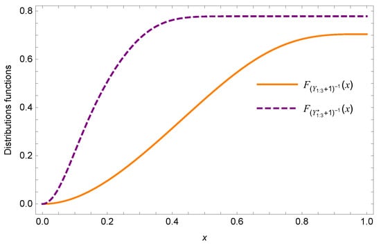
Consider two series systems. Let $G_1\left(x\right)=1-\frac{1}{1+x}$ and $G_2\left(x\right)=e^{-\frac{2}{x}}$ for $x>0$. suppose that $(p_1,p_1,p_3)=(e^{-0.05},e^{-0.08},e^{-0.22})$, $(p_1^{*},p_2^{*},p_3^{*})=(e^{-0.01},e^{-0.21},e^{-0.03})$, $({\beta }_1,{\beta }_2,{\beta }_2)$$=(2,5,6)\stackrel{w}{⪰}(4.5,5,5.8)=({\delta }_1,{\delta }_2,{\delta }_3)$ and $({\alpha }_1,{\alpha }_2,{\alpha }_2)=(1.1,4,6.5)\stackrel{w}{⪰}(3.5,4,6.3)=({\gamma }_1,{\gamma }_2,{\gamma }_3)$. As mentioned in Remark 4, we choose the Clayton copula with generator $\psi \left(x\right)={(\theta x+1)}^{-\frac{1}{\theta }}$ for $\theta \ge 0$, set ${\theta }_1=2$ and ${\theta }_2=4$. Clearly, the conditions of Theorem 3 are satisfied. To plot the whole of distributions functions curves the lifetime of $Y_{1:3}$ and $Y_{1:3}^{*}$ on $[0,\infty )$, we take the transformation ${(x+1)}^{-1}:[0,\infty )\to [0,1]$. Then $Y_{1:3}{\le }_{st}{Y}_{1:3}^{*}$ is equivalent to ${(Y_{1:3}+1)}^{-1}{\ge }_{st}{(Y_{1:3}^{*}+1)}^{-1}$. Figure 1 shows that the distribution of ${(Y_{1:3}^{*}+1)}^{-1}$ is always larger than the distribution of ${(Y_{1:3}+1)}^{-1}$, and this confirms that $Y_{1:3}{\le }_{st}{Y}_{1:3}^{*}$.

Figure 1. Plots of distribution functions of ${(Y_{1:3}+1)}^{-1}$ and ${(Y_{1:3}^{*}+1)}^{-1}$.

The following example shows that the condition ${\varphi }_2\circ {\psi }_1$ is super-additive given that in the above Theorem 3 it cannot be dropped.

Example 2.

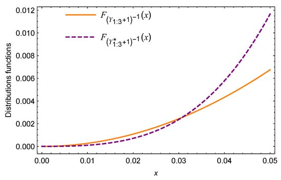
Under the setup of Example 1, let generators ${\psi }_1\left(x\right)={({\theta }_{1}x+1)}^{-\frac{1}{{\theta }_1}}$ and ${\psi }_2\left(x\right)={({\theta }_{2}x+1)}^{-\frac{1}{{\theta }_2}}$ for $\theta \ge 0$. When ${\theta }_1=4$ and ${\theta }_2=0.2$, note that ${\left[{\varphi }_{2}o{\psi }_1\left(t\right)\right]}^{{}^{\prime \prime }}\ngeqq 0$. Thus, the super-additive of ${\varphi }_2\circ {\psi }_1$ is not satisfied. As is seen in Figure 2, ${(Y_{1:3}+1)}^{-1}$ is not always beneath that of ${(Y_{1:3}^{*}+1)}^{-1}$, that is, neither $Y_{1:3}{\ge }_{st}{Y}_{1:3}^{*}$ nor $Y_{1:3}{\le }_{st}{Y}_{1:3}^{*}$.

Figure 2. Plots of distribution functions of ${(Y_{1:3}+1)}^{-1}$ and ${(Y_{1:3}^{*}+1)}^{-1}$.

The next result studies the effects of surviving probabilities from random shocks on the lifetimes of series systems in the sense of the usual stochastic order.

Theorem 4.

Suppose $X_1,X_2,\dots ,X_n$ and $X_1^{*},X_2^{*},\dots ,X_n^{*}$ are two sets of dependent MOTL-G random variables having common Archimedean copula with generator ψ such that $X_i\sim MOTL-G({\alpha }_i,{\beta }_i,G_1\left(x\right))$ and $X_i^{*}\sim MOTL-G({\gamma }_i,{\delta }_i,G_2\left(x\right))$, $i=1,2,\dots ,n$. Further, assume $I_{p_1},I_{p_2},\dots ,$$I_{p_n}$$(I_{p_1^{*}},I_{p_2^{*}},\dots ,I_{p_n^{*}})$ be a set of independent Bernoulli random variables with $E\left(I_{p_i}\right)=p_i\left(E\left(I_{p_i^{*}}\right)=p_i^{*}\right)$, independent of $X_i\prime s\left(X_i^{*}\prime s\right)$, $i=1,2,\dots ,n$. If $Z_1{\le }_{st}{Z}_2$ ${\alpha }_i={\gamma }_{i}and{\beta }_i={\delta }_i(i=1,2,\dots ,n)$, then

$$\prod _{i=1}^n{p}_i\le \prod _{i=1}^n{p}_i^{*}⟹Y_{1:n}{\le }_{st}{Y}_{1:n}^{*}.$$

Proof of Theorem 4.

The survival functions of $Y_{1:n}$ and $Y_{1:n}^{*}$ can be expressed as

$$\begin{array}{c}\hfill \begin{array}{c}\hfill {\overline{F}}_{Y_{1:n}}\left(x\right)=\prod _{i=1}^n{p}_i\psi \left(\sum _{i=1}^n\varphi \left(\zeta ({\alpha }_i,{\beta }_i,G_1\left(x\right))\right)\right),\end{array}\end{array}$$

(7)

and

$$\begin{array}{c}\hfill \begin{array}{c}\hfill {\overline{F}}_{Y_{1:n}^{*}}\left(x\right)=\prod _{i=1}^n{p}_i^{*}\psi \left(\sum _{i=1}^n\varphi \left(\zeta ({\alpha }_i,{\beta }_i,G_2\left(x\right))\right)\right),\end{array}\end{array}$$

(8)

respectively. In order to obtain the required result, it is sufficient to show that ${\overline{F}}_{Y_{1:n}}\left(x\right)\le {\overline{F}}_{Y_{1:n}^{*}}\left(x\right)$. It is equivalent to show that

$$\begin{array}{c}\hfill \begin{array}{c}\hfill \prod _{i=1}^n{p}_i\psi \left(\sum _{i=1}^n\varphi \left(\zeta ({\alpha }_i,{\beta }_i,G_1\left(x\right))\right)\right)\le \prod _{i=1}^n{p}_i^{*}\psi \left(\sum _{i=1}^n\varphi \left(\zeta ({\alpha }_i,{\beta }_i,G_2\left(x\right))\right)\right).\end{array}\end{array}$$

(9)

In view of Lemma 2 and $Z_1{\le }_{st}{Z}_2$, we have $\zeta ({\alpha }_i,{\beta }_i,G_1\left(x\right))\le \zeta ({\alpha }_i,{\beta }_i,G_2\left(x\right))$. Again, the decreasing property of ${\varphi }_1$ and ${\psi }_1$ implies that

$$\psi \left(\sum _{i=1}^n\varphi \left(\zeta ({\alpha }_i,{\beta }_i,G_1\left(x\right))\right)\right)\le \psi \left(\sum _{i=1}^n\varphi \left(\zeta ({\alpha }_i,{\beta }_i,G_2\left(x\right))\right)\right).$$

According to the condition of ${\prod }_{i=1}^n{p}_i\le {\prod }_{i=1}^n{p}_i^{*}$, it is obvious that ${\overline{F}}_{Y_{1:n}}\left(x\right)\le {\overline{F}}_{Y_{1:n}^{*}}\left(x\right)$, that is, $Y_{1:n}{\le }_{st}{Y}_{1:n}^{*}$. □

Remark 5.

Theorem 4 shows that the greater the product of the surviving probabilities from random shocks is, the larger the lifetimes of the series system are. The condition ${\prod }_{i=1}^n{p}_i\le {\prod }_{i=1}^n{p}_i^{*}$ is a weaker condition than $(p_1,p_2,\dots ,p_n)\stackrel{w}{⪰}(p_1^{*},p_2^{*},\dots ,p_n^{*})$, that is, the latter condition implies the former condition.

The following theorem presents sufficient conditions for comparing two series systems with heterogeneous dependent components in terms of the hazard rate ordering.

Theorem 5.

Suppose $X_1,\dots ,X_n$ and $X_1^{*},\dots ,X_n^{*}$ are two sets of dependent MOTL-G random variables having a common Archimedean copula with generator ψ such that $X_i\sim MOTL-G({\alpha }_i,\beta ,G_1)$ and $X_i^{*}\sim MOTL-G({\gamma }_i,\beta ,G_2)$, $i=1,2,\dots ,n$. Further, assume $I_{p_1},\dots ,I_{p_n}$$(I_{p_1^{*}},\dots ,I_{p_n^{*}})$ be a set of independent Bernoulli random variables with $E\left(I_{p_i}\right)=p_i(E\left(I_{p_i^{*}}\right)=p_i^{*})$, independent of $X_i\prime s(X_i^{*}\prime s)$, $i=1,2,\dots ,n$. If

(i)${\prod }_{i=1}^n{p}_i\le {\prod }_{i=1}^n{p}_i^{*}$;

(ii)$\psi$is log-concave; and

(iii)$\psi (1-\psi )/{\psi }^{{}^{\prime }}$is decreasing and concave (or convex), then

$$\left({\alpha }_1,{\alpha }_2,\dots ,{\alpha }_n\right)\stackrel{w}{⪰}\left({\gamma }_1,{\gamma }_2,\dots ,{\gamma }_n\right)⟹Y_{1:n}{\le }_{hr}{Y}_{1:n}^{*}.$$

Proof of Theorem 5.

According to (4), the ratio of the survival functions of $Y_{1:n}^{*}$ and $Y_{1:n}$ can be written as

$$\frac{{\overline{F}}_{Y_{1:n}^{*}}\left(x\right)}{{\overline{F}}_{Y_{1:n}}\left(x\right)}=\left(\frac{{\prod }_{i=1}^n{p}_i^{*}}{{\prod }_{i=1}^n{p}_i}\right)\frac{{\overline{F}}_{X_{1:n}^{*}}\left(x\right)}{{\overline{F}}_{X_{1:n}}\left(x\right)},x\ge 0.$$

In order to obtain the desired result, we need to prove that ${\overline{F}}_{Y_{1:n}^{*}}\left(x\right)/{\overline{F}}_{Y_{1:n}}\left(x\right)$ is increasing in x. It is equivalent to ${\overline{F}}_{X_{1:n}^{*}}\left(x\right)/{\overline{F}}_{X_{1:n}}\left(x\right)$ is increasing in x and

$$\begin{array}{c}\hfill 1=\underset{x\to 0^{-}}{lim}\frac{{\overline{F}}_{Y_{1:n}^{*}}\left(x\right)}{{\overline{F}}_{Y_{1:n}}\left(x\right)}\le \frac{{\overline{F}}_{Y_{1:n}^{*}}\left(0\right)}{{\overline{F}}_{Y_{1:n}}\left(0\right)}=\frac{{\prod }_{i=1}^n{p}_i^{*}}{{\prod }_{i=1}^n{p}_i}.\end{array}$$

(10)

It is obvious that Inequality (10) holds according to the assumptions. Note that the hazard rate function of $X_{1:n}$ is given by

$$\begin{array}{ccc}\hfill r_{X_{1:n}}\left(x\right)& =& \frac{2\beta g\left(x\right)\overline{G}\left(x\right)}{\left(1-{\overline{G}}^2\left(x\right)\right)\left[1-{\left(1-{\overline{G}}^2\left(x\right)\right)}^{\beta }\right]}\frac{{\psi }^{\prime }\left(\sum _{i=1}^n\varphi \left(\zeta ({\alpha }_i,\beta ,G\left(x\right))\right)\right)}{\psi \left(\sum _{i=1}^n\varphi \left(\zeta ({\alpha }_i,\beta ,G\left(x\right))\right)\right)}\hfill \\ & & \times \sum _{i=1}^n\frac{\psi \left(\varphi \left(\zeta ({\alpha }_i,\beta ,G\left(x\right))\right)\right)}{{\psi }^{\prime }\left(\varphi \left(\zeta ({\alpha }_i,\beta ,G\left(x\right))\right)\right)}(1-\zeta ({\alpha }_i,\beta ,G\left(x\right))).\hfill \end{array}$$

Clearly, $r_{X_{1:n}}\left(x\right)$ is permutation-symmetric with respect to $({\alpha }_1,{\alpha }_2,\dots ,{\alpha }_n)$, which implies that $r_{X_{1:n}}\left(x\right)$ is a symmetric function. Then, the desired result follows if $X_{1:n}{\le }_{hr}{X}_{1:n}^{*}$. Now, it is enough to show that $r_{X_{1:n}}\left(x\right)$ is decreasing in ${\alpha }_i$ and Schur-convex in $\alpha =({\alpha }_1,{\alpha }_2,\dots ,{\alpha }_n)$. The rest of the proof is similar to that of Theorem 3.3 of Panja et al. [29] and is therefore omitted here. □

Remark 6.

Note that without any restriction on surviving probabilities from random shocks, Theorem 5.3 of Panja et al. [29] showed that $\mathbf{\alpha }\stackrel{\mathrm{w}}{⪰}\gamma$ implies $Y_{1:n}{\le }_{hr}{Y}_{1:n}^{*}$. However, their result is not correct as they neglected the value of the survival ratio function ${\overline{F}}_{Y_{1:n}^{*}}\left(x\right)/{\overline{F}}_{Y_{1:n}}\left(x\right)$ at point $x=0$. Fortunately, this could be corrected according to the proof method of Theorem 5.

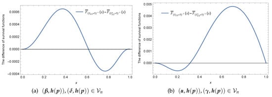
The following example shows that one may not get the ordering result in Theorem 5 if the condition of ${\prod }_{i=1}^n{p}_i\le {\prod }_{i=1}^n{p}_i^{*}$ is removed.

Example 3.

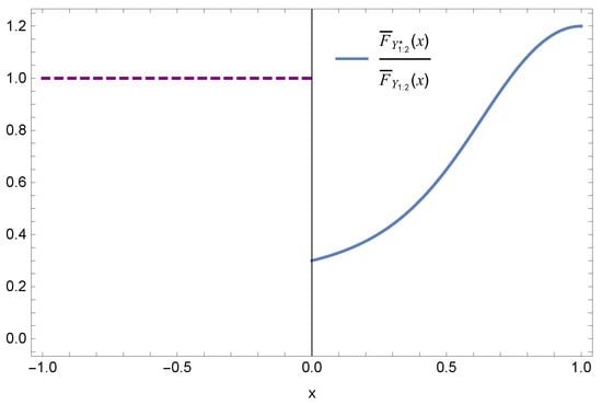
Consider the case of $n=2$. Let $G\left(x\right)=x$, $0\le x\le 1$, and generator $\psi \left(x\right)=2/(1+e^x)$. Set $\beta =1$, ${\alpha }_1=2$, ${\alpha }_2=3$, ${\gamma }_1=4$, ${\gamma }_2=6$, and ${\prod }_{i=1}^n{p}_i^{*}/{\prod }_{i=1}^n{p}_i=0.3$. However, ${\overline{F}}_{Y_{1:2}^{*}}\left(x\right)/{\overline{F}}_{Y_{1:2}}\left(x\right)$ is not monotone (see Figure 3). Therefore, the condition of ${\prod }_{i=1}^n{p}_i\le {\prod }_{i=1}^n{p}_i^{*}$ cannot be removed.

Figure 3. The ratio of survival functions $Y_{1:2}^{*}$ and $Y_{1:2}$.

Naturally, one may wonder whether the hazard rate order actually holds in between $Y_{1:n}$ and $Y_{1:n}^{*}$ when $\beta \stackrel{\mathrm{w}}{⪰}\delta$ for fixed shape parameter $\alpha$. Unfortunately, Example 4 gives a negative answer even for the independent case.

Example 4.

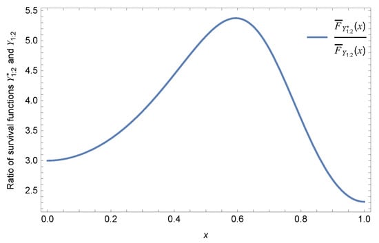
Let $G\left(x\right)=x$ and $0\le x\le 1$; it is assumed that $\alpha =1.2$, ${\beta }_1=2$, ${\beta }_2=7$, ${\delta }_1=6$, ${\delta }_2=9$ and ${\prod }_{i=1}^n{p}_i^{*}/{\prod }_{i=1}^n{p}_i=3$. As is displayed in Figure 4, ${\overline{F}}_{Y_{1:2}^{*}}\left(x\right)/{\overline{F}}_{Y_{1:2}}\left(x\right)$ is not monotone in x. Therefore, neither of $Y_{1:2}{\ge }_{hr}{Y}_{1:2}^{*}$ and $Y_{1:2}{\le }_{hr}{Y}_{1:2}^{*}$ is true.

Figure 4. The ratio of survival functions $Y_{1:2}^{*}$ and $Y_{1:2}$.

3.1.2. Comparison of Two Parallel Systems

In this subsection, we carry out stochastic comparison of parallel systems with dependent heterogeneous components in the sense of usual stochastic ordering. In the following, we study the effect of heterogeneity among surviving probabilities from random shocks on the reliabilities of parallel system.

Theorem 6.

Let $X_1,\dots ,X_n$$(X_1^{*},\dots ,X_n^{*})$ be a set of independent MOTL-G random variables such that $X_i\sim MOTL-G({\alpha }_i,{\beta }_i,G_1\left(x\right))$$(X_i^{*}\sim MOTL-G({\alpha }_i,{\beta }_i,G_2\left(x\right)))$, $i=1,2$. Further, assume $I_{p_1},\dots ,I_{p_n}$$(I_{p_1^{*}},\dots ,I_{p_n^{*}})$ be a set of independent Bernoulli random variables with $E\left(I_{p_i}\right)=p_i(E\left(I_{p_i^{*}}\right)=p_i^{*})$, independent of $X_i\prime s(X_i^{*}\prime s)$, $i=1,2$. If

(i)$Z_1{\ge }_{st}{Z}_2$,

(ii)$(\mathbf{\alpha },\mathbf{\beta })\in {\mathcal{U}}_2$, $(\mathbf{\beta },\mathit{h}\left(\mathit{p}\right))\in {\mathcal{V}}_2$and$(\mathbf{\beta },\mathit{h}\left({\mathbf{p}}^{*}\right))\in {\mathcal{V}}_2$and

(iii)$h:[0,1]\to (0,\infty )$is a differentiable and strictly decreasing convex function, then

$$(h\left(p_1\right),h\left(p_2\right))\stackrel{\mathrm{w}}{⪰}(h\left(p_1^{*}\right),h\left(p_2^{*}\right))⟹Y_{2:2}{\ge }_{st}{Y}_{2:2}^{*}.$$

Proof of Theorem 6.

The distribution function of $Y_{2:2}$ can be written as

$$\begin{array}{c}\hfill \begin{array}{cc}\hfill F_{Y_{2:2}}\left(x\right)=& 1-P(Y_{2:2}>x)\hfill \\ \hfill =& 1-P(Y_1>x)-P(Y_2>x)+P(Y_1>x,Y_2>x)\hfill \\ \hfill =& 1-P(X_1{I}_{p_1}>x|I_{p_1}=1)p_1-P(X_2{I}_{p_2}>x|I_{p_2}=1)p_2\hfill \\ & +P(X_1{I}_{p_1}>x,X_2{I}_{p_2}>x|I_{p_1}=1,I_{p_2}=1)p_1{p}_2\hfill \\ & +P(X_1{I}_{p_1}>x,X_2{I}_{p_2}>x|I_{p_1}=1,I_{p_2}=0)p_1(1-p_2)\hfill \\ & +P(X_1{I}_{p_1}>x,X_2{I}_{p_2}>x|I_{p_1}=0,I_{p_2}=1)(1-p_1)p_2\hfill \\ & +P(X_1{I}_{p_1}>x,X_2{I}_{p_2}>x|I_{p_1}=0,I_{p_2}=0)(1-p_1)(1-p_2)\hfill \\ \hfill =& 1-h^{-1}\left(u_1\right){\overline{F}}_{X_1}\left(x\right)-h^{-1}\left(u_2\right){\overline{F}}_{X_2}\left(x\right)+h^{-1}\left(u_1\right)h^{-1}\left(u_2\right){\overline{F}}_{X_{1:2}}\left(x\right)\hfill \\ \hfill :=& \Psi ({\alpha }_1,{\alpha }_2,{\beta }_1,{\beta }_2,p_1,p_2,\psi ,G_1\left(x\right)),\hfill \end{array}\end{array}$$

where ${\overline{F}}_{X_{1:2}}\left(x\right)=\psi \left(\sum _{i=1}^2\varphi \left(\frac{{\alpha }_i\left(1-{\left(1-{\left(1-G_1\left(x\right)\right)}^2\right)}^{{\beta }_i}\right)}{{\alpha }_i+{\overline{\alpha }}_i{\left(1-{\left(1-G_1\left(x\right)\right)}^2\right)}^{{\beta }_i}}\right)\right)$, ${\overline{F}}_{X_i}\left(x\right)=\frac{{\alpha }_i\left(1-{\left(1-{\left(1-G_1\left(x\right)\right)}^2\right)}^{{\beta }_i}\right)}{{\alpha }_i+{\overline{\alpha }}_i{\left(1-{\left(1-G_1\left(x\right)\right)}^2\right)}^{{\beta }_i}}$ and $p_i=h^{-1}\left(u_i\right),$$i=1,2$. Similarly, $F_{Y_{2:2}^{*}}\left(x\right)=\Psi ({\alpha }_1,{\alpha }_2,{\beta }_1,{\beta }_2,p_1^{*},p_2^{*},\psi ,G_2\left(x\right)).$ The required result is equivalent to $F_{Y_{2:2}}\left(x\right)\le F_{Y_{2:2}^{*}}\left(x\right)$. It is obvious that ${\overline{F}}_{X_{1:2}}\left(x\right)$ is increasing in G and ${\overline{F}}_{X_i}\left(x\right)$ is decreasing in $G,$ thus

$$\mathrm{\Psi }({\alpha }_1,{\alpha }_2,{\beta }_1,{\beta }_2,p_1^{*},p_2^{*},\psi ,G_1\left(x\right))\le \mathrm{\Psi }({\alpha }_1,{\alpha }_2,{\beta }_1,{\beta }_2,p_1^{*},p_2^{*},\psi ,G_2\left(x\right)),$$

when $Z_1{\ge }_{st}{Z}_2.$ Thus, we only need to prove

$$\mathrm{\Psi }({\alpha }_1,{\alpha }_2,{\beta }_1,{\beta }_2,p_1,p_2,\psi ,G_1\left(x\right))\le \mathrm{\Psi }({\alpha }_1,{\alpha }_2,{\beta }_1,{\beta }_2,p_1^{*},p_2^{*},\psi ,G_1\left(x\right)).$$

For ${\beta }_1={\beta }_2=\dots ={\beta }_n$ and ${\alpha }_1={\alpha }_2=\dots ={\alpha }_n$, $F_{Y_{2:2}}$ is symmetric with respect to $(u_1,u_2)$. When ${\beta }_i$ and ${\alpha }_i$ are variable, it implies that $F_{Y_{2:2}}$ is asymmetric with respect to $(u_1,u_2)$. Without loss of generality, assume that ${\alpha }_1\ge {\alpha }_2$ and ${\beta }_1\ge {\beta }_2$. For $(\mathbf{\beta },\mathit{h}(\mathit{p}\left)\right)$ and $(\mathbf{\beta },\mathit{h}\left({\mathit{p}}^{*}\right))\in {\mathcal{V}}_2$, then it is obvious that $h\left(p_1\right)\le h\left(p_2\right)$ and $h\left(p_1^{*}\right)\le h\left(p_2^{*}\right)$. Define $\Phi \left(\mathit{u}\right)=-F_{Y_{2:2}}\left(x\right)$. Then, the partial derivatives of $\mathrm{\Phi }\left(\mathit{u}\right)$ with respect to $u_1$ and $u_2$ can be expressed as

$$\begin{array}{c}\hfill \frac{\partial \mathrm{\Phi }\left(\mathit{u}\right)}{\partial u_1}=\frac{\mathrm{d}{h}^{-1}\left(u_1\right)}{\mathrm{d}{u}_1}\left[{\overline{F}}_{X_1}\left(x\right)-h^{-1}\left(u_2\right){\overline{F}}_{X_{1:2}}\left(x\right)\right]\le 0,\end{array}$$

and

$$\begin{array}{c}\hfill \frac{\partial \Phi \left(\mathit{u}\right)}{\partial u_2}=\frac{\mathrm{d}{h}^{-1}\left(u_2\right)}{\mathrm{d}{u}_2}\left[{\overline{F}}_{X_2}\left(x\right)-h^{-1}\left(u_2\right){\overline{F}}_{X_{1:2}}\left(x\right)\right]\le 0,\end{array}$$

where the above inequalities are owing to the decreasing property of $h^{-1}$ and the non-negativity of ${\overline{F}}_{X_i}\left(x\right)-{\overline{F}}_{X_{1:2}}\left(x\right)$, $i=1,2$. Thus, $\Phi \left(\mathit{u}\right)$ is decreasing with respect to $u_i$, $i=1,2$. On the other hand, it is easy to check that ${\overline{F}}_{X_i}\left(x\right)$ is increasing in ${\alpha }_i$ and ${\beta }_i$, $i=1,2$. For ${\alpha }_1\ge {\alpha }_2$ and ${\beta }_1\ge {\beta }_2$, we have

$$\begin{array}{c}\hfill \begin{array}{c}\hfill {\overline{F}}_{X_1}\left(x\right)\ge {\overline{F}}_{X_2}\left(x\right).\end{array}\end{array}$$

(11)

Now, for any $u_1\le u_2$, we have

$$\begin{array}{c}\hfill \begin{array}{cc}& \left(\frac{\partial \Phi \left(\mathit{u}\right)}{\partial u_1}-\frac{\partial \Phi \left(\mathit{u}\right)}{\partial u_2}\right)\hfill \\ \hfill =& \frac{\mathrm{d}{h}^{-1}\left(u_1\right)}{\mathrm{d}{u}_1}\left[{\overline{F}}_{X_1}\left(x\right)-h^{-1}\left(u_2\right){\overline{F}}_{X_{1:2}}\left(x\right)\right]-\frac{\mathrm{d}{h}^{-1}\left(u_2\right)}{\mathrm{d}{u}_2}\left[{\overline{F}}_{X_2}\left(x\right)-h^{-1}\left(u_1\right){\overline{F}}_{X_{1:2}}\left(x\right)\right]\hfill \\ \hfill =& \frac{\mathrm{d}{h}^{-1}\left(u_1\right)}{\mathrm{d}{u}_1}\left[{\overline{F}}_{X_1}\left(x\right)-h^{-1}\left(u_2\right){\overline{F}}_{X_{1:2}}\left(x\right)\right]-\frac{\mathrm{d}{h}^{-1}\left(u_2\right)}{\mathrm{d}{u}_2}\left[{\overline{F}}_{X_1}\left(x\right)-h^{-1}\left(u_2\right){\overline{F}}_{X_{1:2}}\left(x\right)\right]\hfill \\ & +\frac{\mathrm{d}{h}^{-1}\left(u_2\right)}{\mathrm{d}{u}_2}\left[{\overline{F}}_{X_1}\left(x\right)-h^{-1}\left(u_2\right){\overline{F}}_{X_{1:2}}\left(x\right)\right]-\frac{\mathrm{d}{h}^{-1}\left(u_2\right)}{\mathrm{d}{u}_2}\left[{\overline{F}}_{X_2}\left(x\right)-h^{-1}\left(u_1\right){\overline{F}}_{X_{1:2}}\left(x\right)\right]\hfill \\ \hfill =& \left[\left({\overline{F}}_{X_1}\left(x\right)-{\overline{F}}_{X_2}\left(x\right)\right)+(h^{-1}\left(u_1\right)-h^{-1}\left(u_2\right)){\overline{F}}_{X_{1:2}}\left(x\right)\right]\frac{\mathrm{d}{h}^{-1}\left(u_2\right)}{\mathrm{d}{u}_2}\hfill \\ & +\left(\frac{\mathrm{d}{h}^{-1}\left(u_1\right)}{\mathrm{d}{u}_1}-\frac{\mathrm{d}{h}^{-1}\left(u_2\right)}{\mathrm{d}{u}_2}\right)\times \left[{\overline{F}}_{X_1}\left(x\right)-h^{-1}\left(u_2\right){\overline{F}}_{X_{1:2}}\left(x\right)\right].\hfill \end{array}\end{array}$$

Because h is strictly decreasing and convex, $h^{-1}$ is also strictly decreasing and convex. Thus, we have

$$\begin{array}{c}\hfill \begin{array}{c}\hfill \frac{\mathrm{d}{h}^{-1}\left(u_1\right)}{\mathrm{d}{u}_1}\le \frac{\mathrm{d}{h}^{-1}\left(u_2\right)}{\mathrm{d}{u}_2}<0,\end{array}\end{array}$$

(12)

and

$$\begin{array}{c}\hfill \begin{array}{c}\hfill h^{-1}\left(u_1\right)\ge h^{-1}\left(u_2\right),\end{array}\end{array}$$

(13)

Now, upon combining (11)–(13), we get

$$\left(\frac{\partial \Phi \left(\mathit{u}\right)}{\partial u_1}-\frac{\partial \Phi \left(\mathit{u}\right)}{\partial u_2}\right)\le 0.$$

It follows from Lemma 5 that $\mathrm{\Phi }\left(\mathit{u}\right)$ is Schur-convex. Then, the desired result obtained from Lemma 6. □

Remark 7.

In accordance with Theorem 6, we conclude that more heterogeneity among the transformations of surviving probabilities from random shocks, according to the weak majorization order, implies larger lifetime of the parallel systems consisting of two dependent heterogeneous components in the sense of the usual stochastic order. It might be of great interest to study the effect of the heterogeneity of shape parameters on parallel systems in the sense of usual stochastic order, which is left as a future problem.

3.2. Comparison of Two Parallel Systems in Heterogeneous Independent Case

In this subsection, we discuss the usual stochastic order of parallel systems with independent heterogeneous MOTL-G components associated random shocks. Next, we study the influence of heterogeneity of surviving probabilities from random shocks and shape parameters on the lifetime of parallel systems in Theorems 7 and 8, respectively. The distribution functions of $Y_{n:n}$ and $Y_{n:n}^{*}$ are given by

$$\begin{array}{c}\hfill \begin{array}{cc}\hfill F_{Y_{n:n}}\left(x\right)& =\prod _{i=1}^n{F}_{Y_i}\left(x\right)=\prod _{i=1}^n\left[1-h^{-1}\left(u_i\right)\frac{{\alpha }_i\left(1-{\left(1-{\left(1-G_1\left(x\right)\right)}^2\right)}^{{\beta }_i}\right)}{{\alpha }_i+{\overline{\alpha }}_i{\left(1-{\left(1-G_1\left(x\right)\right)}^2\right)}^{{\beta }_i}}\right]\hfill \\ & =\prod _{i=1}^n\left[1-h^{-1}\left(u_i\right)\zeta ({\alpha }_i,{\beta }_i,G_1\left(x\right))\right]\hfill \\ & =J(\mathit{u},\alpha ,\beta ,G_1\left(x\right)),\hfill \end{array}\end{array}$$

(14)

and

$$\begin{array}{c}\hfill \begin{array}{cc}\hfill F_{Y_{n:n}^{*}}\left(x\right)& =\prod _{i=1}^n{F}_{Y_i}\left(x\right)=\prod _{i=1}^n\left[1-h^{-1}\left(u_i^{*}\right)\frac{{\gamma }_i\left(1-{\left(1-{\left(1-G_2\left(x\right)\right)}^2\right)}^{{\delta }_i}\right)}{{\gamma }_i+{\overline{\gamma }}_i{\left(1-{\left(1-G_2\left(x\right)\right)}^2\right)}^{{\delta }_i}}\right]\hfill \\ & =\prod _{i=1}^n\left[1-h^{-1}\left(u_i^{*}\right)\zeta ({\gamma }_i,{\delta }_i,G_2\left(x\right))\right]\hfill \\ & =J({\mathit{u}}^{*},\gamma ,\delta ,G_2\left(x\right)),\hfill \end{array}\end{array}$$

(15)

where $u_i=h\left(p_i\right)$, $u_i^{*}=h\left(p_i^{*}\right)$, $\alpha =({\alpha }_1,\dots ,{\alpha }_n)$, $\beta =({\beta }_1,\dots ,{\beta }_n)$, $\gamma =({\gamma }_1,\dots ,{\gamma }_n)$, and $\delta =({\delta }_1,\dots ,{\delta }_n)$. For $x=0$, the distributed functions of $Y_{n:n}$ and $Y_{n:n}^{*}$ are given by $F_{Y_{n:n}}\left(0\right)={\prod }_{i=1}^n\left(1-p_i\right)$ and $F_{Y_{n:n}^{*}}\left(0\right)={\prod }_{i=1}^n\left(1-p_i^{*}\right)$.

Theorem 7.

Suppose $X_1,\dots ,X_n$$(X_1^{*},\dots ,X_n^{*})$ is a set of independent MOTL-G random variables such that $X_i\sim MOTL-G({\alpha }_i,{\beta }_i,G_1\left(x\right))$$(X_i^{*}\sim MOTL-G({\alpha }_i,{\beta }_i,G_2\left(x\right)))$, $i=1,2,\dots ,n$. Further, assume $I_{p_1},\dots ,I_{p_n}$$(I_{p_1^{*}},\dots ,I_{p_n^{*}})$ is a set of independent Bernoulli random variables with $E\left(I_{p_i}\right)=p_i(E\left(I_{p_i^{*}}\right)=p_i^{*})$, independent of $X_i\prime s(X_i^{*}\prime s)$, $i=1,2,\dots ,n$. If

(i)$Z_1{\ge }_{st}{Z}_2$;

(ii)$(\mathbf{\alpha },\mathbf{\beta })\in {\mathcal{U}}_n$, $(\beta ,\mathit{h}\left(\mathit{p}\right))\in {\mathcal{V}}_n$, and$(\beta ,\mathit{h}\left({\mathit{p}}^{*}\right))\in {\mathcal{V}}_n$; and

(iii)$h:[0,1]\to (0,\infty )$is differentiable and strictly decreasing convex function, then

$$\prod _{i=1}^n(1-p_i)\le \prod _{i=1}^n(1-p_i^{*}),\mathit{h}\left(\mathit{p}\right)\stackrel{w}{⪰}\mathit{h}\left({\mathit{p}}^{*}\right)⟹Y_{n:n}{\ge }_{st}{Y}_{n:n}^{*}.$$

Proof of Theorem 7.

Without loss of generality, assume that $\mathbf{\alpha }\in {\mathcal{D}}_{+}$ and $\mathbf{\beta }\in {\mathcal{D}}_{+}$. For $(\mathbf{\beta },\mathit{h}(\mathit{p}\left)\right)$ and $(\mathbf{\beta },\mathit{h}\left({\mathit{p}}^{*}\right))\in {\mathcal{V}}_n$, then it is obvious that $\mathit{h}\left(\mathit{p}\right)\in {\mathcal{E}}_{+}$ and $\mathit{h}\left({\mathit{p}}^{*}\right)\in {\mathcal{E}}_{+}$. Under random shock, denote $T_i^{*}=X_i{I}_{p_i^{*}}$, then the distribution functions of $T_{n:n}^{*}$ are given by

$$\begin{array}{c}\hfill F_{T_{n:n}^{*}}\left(x\right)=\prod _{i=1}^n\left[1-h^{-1}\left(u_i^{*}\right)\zeta ({\alpha }_i,{\beta }_i,G_1\left(x\right))\right]=J({\mathit{u}}^{*},\mathbf{\alpha },\mathbf{\beta },G_1\left(x\right)).\end{array}$$

To obtain the required result, it suffices to show that $F_{Y_{n:n}}\le F_{Y_{n:n}^{*}}$, that is,

$$J(\mathit{u},\mathbf{\alpha },\mathbf{\beta },G_1\left(x\right))\le J({\mathit{u}}^{*},\mathbf{\alpha },\mathbf{\beta },G_2\left(x\right)).$$

For ${\beta }_1={\beta }_2=\dots ={\beta }_n$ and ${\alpha }_1={\alpha }_2=\dots ={\alpha }_n$, $J(\mathit{u},\mathbf{\alpha },\mathbf{\beta },G_1\left(x\right))$ is symmetric in $\mathit{u}$. For ${\beta }_1\ne {\beta }_2\ne \dots \ne {\beta }_n$ and ${\alpha }_1\ne {\alpha }_2\ne \dots \ne {\alpha }_n$, $J(\mathit{u},\mathbf{\alpha },\mathbf{\beta },G_1\left(x\right))$ is asymmetric in $\mathit{u}$. Note that $Z_1{\ge }_{st}{Z}_2$ implies $G_1\left(x\right)\le G_2\left(x\right)$ for $x\ge 0$, and $\zeta ({\alpha }_i,{\beta }_i,G_i\left(x\right))$ is decreasing in $G_i\left(x\right)$ for $i=1,2$, which yields

$$\zeta ({\alpha }_i,{\beta }_i,G_1\left(x\right))\ge \zeta ({\alpha }_i,{\beta }_i,G_2\left(x\right)),$$

which in turn implies that

$$\begin{array}{c}\hfill J({\mathit{u}}^{*},\mathbf{\alpha },\mathbf{\beta },G_1\left(x\right))\le J({\mathit{u}}^{*},\mathbf{\alpha },\mathbf{\beta },G_2\left(x\right)).\end{array}$$

Thus, it is enough to show that

$$J(\mathit{u},\mathbf{\alpha },\mathbf{\beta },G_1\left(x\right))\le J({\mathit{u}}^{*},\mathbf{\alpha },\mathbf{\beta },G_1\left(x\right)).$$

When $x=0$, the desired result follows immediately from the assumption $\prod _{i=1}^n(1-p_i)\le \prod _{i=1}^n(1-p_i^{*})$. When $x>0$, by Lemma 6, it is enough to show that $J(\mathit{u},\mathbf{\alpha },\mathbf{\beta },G_1\left(x\right))$ is increasing and Schur-concave. Taking the partial derivative of $J(\mathit{u},\mathbf{\alpha },\mathbf{\beta },G_1\left(x\right))$ with respect to $u_i$, we have

$$\begin{array}{c}\hfill \frac{\partial J(\mathit{u},\mathbf{\alpha },\mathbf{\beta },G_1\left(x\right))}{\partial u_i}=\left[-\frac{d{h}^{-1}\left(u_i\right)}{d{u}_i}\zeta ({\alpha }_i,{\beta }_i,G_1\left(x\right))\right]\times \prod _{k\ne i}^n\left[1-h^{-1}\left(u_k\right)\zeta ({\alpha }_k,{\beta }_k,G_1\left(x\right))\right]\ge 0,\end{array}$$

where the inequality is due to the decreasing properties of $h^{-1}$. Consider that,

$$\begin{array}{c}\hfill \begin{array}{cc}& \frac{\partial J(\mathit{u},\mathbf{\alpha },\mathbf{\beta },G_1\left(x\right))}{\partial u_i}-\frac{\partial J(\mathit{u},\mathbf{\alpha },\mathbf{\beta },G_1\left(x\right))}{\partial u_j}\hfill \\ \hfill \stackrel{\mathrm{sgn}}{=}& \left[-\frac{d{h}^{-1}\left(u_i\right)}{d{u}_i}\zeta ({\alpha }_i,{\beta }_i,G_1\left(x\right))\left(1-h^{-1}\left(u_j\right)\zeta ({\alpha }_j,{\beta }_j,G_1\left(x\right))\right)\right]\hfill \\ & -\left[-\frac{d{h}^{-1}\left(u_j\right)}{d{u}_j}\zeta ({\alpha }_j,{\beta }_j,G_1\left(x\right))\left(1-h^{-1}\left(u_i\right)\zeta ({\alpha }_i,{\beta }_i,G_1\left(x\right))\right)\right],\hfill \end{array}\end{array}$$

(16)

and ${\alpha }_i\ge {\alpha }_j,{\beta }_i\ge {\beta }_j$, $u_i\le u_j$ for any $1\le i\le j\le n$. From Lemma 2, we conclude that

$$\zeta ({\alpha }_i,{\beta }_i,G_1\left(x\right))\ge \zeta ({\alpha }_j,{\beta }_j,G_1\left(x\right)).$$

Based on the condition that $h\left(u\right)$ is decreasing and convex in u, for $u_i\le u_j$, we have

$$\begin{array}{c}\hfill \begin{array}{c}\hfill -\frac{d{h}^{-1}\left(u_i\right)}{d{u}_i}\zeta ({\alpha }_i,{\beta }_i,G_1\left(x\right))\ge -\frac{d{h}^{-1}\left(u_j\right)}{d{u}_j}\zeta ({\alpha }_j,{\beta }_j,G_1\left(x\right)),\end{array}\end{array}$$

(17)

and

$$\begin{array}{c}\hfill 1-h^{-1}\left(u_i\right)\zeta ({\alpha }_i,{\beta }_i,G_1\left(x\right))\le 1-h^{-1}\left(u_j\right)\zeta ({\alpha }_j,{\beta }_j,G_1\left(x\right)).\end{array}$$

(18)

Substituting the results Equations (17) and (18) in Equation (16), for $1\le i<j\le n$, we obtain

$$\frac{\partial J(\mathit{u},\mathbf{\alpha },\mathbf{\beta },G_1\left(x\right))}{\partial u_i}-\frac{\partial J(\mathit{u},\mathbf{\alpha },\mathbf{\beta },G_1\left(x\right))}{\partial u_j}\ge 0.$$

Therefore, the Schur-concave of $J(\mathit{u},\mathbf{\alpha },\mathbf{\beta },G_1\left(x\right))$ can be obtained by Lemma 5. The desired result follows immediately from Lemma 6. □

Remark 8.

Note that the condition of h is differentiable and it is a strictly decreasing convex function that can be easily verified for many functions. For example, $h\left(p\right)=-log\left(p\right)$ and $h\left(p\right)=p^{-\alpha }$, $0<p\le 1$, $\alpha >0$.

Theorem 8.

Let $X_1,\dots ,X_n$$(X_1^{*},\dots ,X_n^{*})$ be a set of independent MOTL-G random variables such that $X_i\sim MOTL-G({\alpha }_i,{\beta }_i,G_1\left(x\right))$$(X_i^{*}\sim MOTL-G({\gamma }_i,{\delta }_i,G_2\left(x\right)))$, $i=1,2,\dots ,n$. Further assume $I_{p_1},\dots ,I_{p_n}$ be a set of independent Bernoulli random variables with $E\left(I_{p_i}\right)=p_i$, independent of $X_i\prime s(X_i^{*}\prime s)$, $i=1,2,\dots ,n$. If $Z_1{\le }_{st}{Z}_2$ and $h:[0,1]\to (0,\infty )$ is a differentiable and decreasing function. Then,

(i) for${\alpha }_i={\gamma }_i=\alpha \ge 1(i=1,2,\dots ,n)$and$(\mathbf{\beta },\mathit{h}\left(\mathit{p}\right)),(\mathbf{\delta },\mathit{h}\left(\mathit{p}\right))\in {\mathcal{U}}_n$, we have

$$\mathbf{\beta }\stackrel{\mathrm{w}}{⪰}\delta ⟹Y_{n:n}{\le }_{st}{Y}_{n:n}^{*};$$

(ii) for${\beta }_i={\gamma }_i=\beta (i=1,2,\dots ,n)$and$(\alpha ,\mathit{h}\left(\mathit{p}\right)),(\gamma ,\mathit{h}\left(\mathit{p}\right))\in {\mathcal{U}}_n$, we have

$$\mathbf{\alpha }\stackrel{\mathrm{w}}{⪰}\gamma ⟹Y_{n:n}{\le }_{st}{Y}_{n:n}^{*};$$

Proof of Theorem 8.

First, assume that $\mathbf{\beta }\in {\mathcal{E}}_{+}$ and $\mathit{h}\left(\mathit{p}\right)\in {\mathcal{E}}_{+}$. Similar to the arguments in the proof of Theorem 7, we notice that to prove the present theorem, it enough to show that

$$J(\mathit{u},\alpha ,\mathbf{\beta },G_1\left(x\right))\ge J(\mathit{u},\alpha ,\delta ,G_1\left(x\right)).$$

Thus, we just need to prove that $J(\mathit{u},\alpha ,\beta ,G_1\left(x\right))$ is decreasing and Schur-convex in $\beta$. When $u_1=u_2=\dots =u_n$, $J(\mathit{u},\alpha ,\mathbf{\beta },G_1\left(x\right))$ is symmetric; otherwise, it is asymmetric. Taking the partial derivative of $J(\mathit{u},\alpha ,\mathbf{\beta },G_1\left(x\right))$ with respect to ${\beta }_i$, we have

$$\begin{array}{ccc}\hfill \frac{\partial J(\mathit{u},\mathbf{\alpha },\mathbf{\beta },G_1\left(x\right))}{\partial {\beta }_i}& =& \left[h^{-1}\left(u_i\right)\frac{\alpha log\left(1-{\left(1-G_1\left(x\right)\right)}^2\right){\left(1-{\left(1-G_1\left(x\right)\right)}^2\right)}^{{\beta }_i}}{{\left(\alpha +\overline{\alpha }{\left(1-{\left(1-G_1\left(x\right)\right)}^2\right)}^{{\beta }_i}\right)}^2}\right]\hfill \\ & & \times \prod _{k\ne i}^n\left[1-h^{-1}\left(u_k\right)\zeta (\alpha ,{\beta }_k,G_1\left(x\right))\right]\le 0,\hfill \end{array}$$

where $\zeta$ is the function defined as in Lemma 2. Therefotr, $J(\mathit{u},\alpha ,\mathbf{\beta },G_1\left(x\right))$ is decreasing in each ${\beta }_i$. Furthermore, for $1\le i<j\le n$, we have

$$\begin{array}{ccc}\hfill \frac{\partial J(\mathit{u},\alpha ,\mathbf{\beta },G_1\left(x\right))}{\partial {\beta }_i}-\frac{\partial J(\mathit{u},\alpha ,\mathbf{\beta },G_1\left(x\right))}{\partial {\beta }_j}& \stackrel{\mathrm{sgn}}{=}& \left(\vartheta (u_i,{\beta }_i)-\vartheta (u_j,{\beta }_j)\right)\hfill \\ & & \times \alpha log\left(1-{\left(1-G_1\left(x\right)\right)}^2\right)\hfill \end{array}$$

(19)

where

$$\vartheta (u,\beta )=\frac{h^{-1}\left(u\right){\left(1-{(1-G_1\left(x\right))}^2\right)}^{\beta }}{{\left(\alpha +\overline{\alpha }{\left(1-{(1-G_1\left(x\right))}^2\right)}^{\beta }\right)}^2\left(1-h^{-1}\left(u\right)\zeta (\alpha ,\beta ,G_1\left(x\right))\right)}.$$

Consider that,

$$\begin{array}{ccc}\hfill \frac{\partial \vartheta (u,\beta )}{\partial \beta }& \stackrel{sgn}{=}& log\left(1-{(1-G_1\left(x\right))}^2\right)\left[{\alpha }^2\left(1-h^{-1}\left(u\right)\right)\left(1-{\left(1-{(1-G_1\left(x\right))}^2\right)}^{2\beta }\right)\right.\hfill \\ & & \left.+{\left(1-{(1-G_1\left(x\right))}^2\right)}^{2\beta }\left(\alpha \left(2-h^{-1}\left(u\right)\right)-1\right)\right]\le 0,\hfill \end{array}$$

which implies $\vartheta (u,\beta )$ is decreasing in $\beta$ for $\alpha \ge 1$. On the other hand, $h\left(u\right)$ is decreasing in u, then

$$\begin{array}{c}\hfill \frac{\partial \vartheta (u,\beta )}{\partial u}\stackrel{sgn}{=}\frac{\mathrm{d}{h}^{-1}\left(u\right)}{\mathrm{d}u}\le 0,\end{array}$$

which implying that $\vartheta (u,\beta )$ is decreasing in u. Thus, for ${\beta }_i\le {\beta }_j$ and $u_i\le u_j$, we conclude that

$$\begin{array}{c}\hfill \begin{array}{c}\hfill \vartheta (u_j,{\beta }_j)\le \vartheta (u_j,{\beta }_i)\le \vartheta (u_i,{\beta }_i).\end{array}\end{array}$$

(20)

Substituting the results Equation (20) in Equation (19), we get

$$\frac{\partial J(\mathit{u},\alpha ,\mathbf{\beta },G_1\left(x\right))}{\partial {\beta }_i}-\frac{\partial J(\mathit{u},\alpha ,\mathbf{\beta },G_1\left(x\right))}{\partial {\beta }_j}\le 0.$$

It follows from Lemma 5 that $J(\mathit{u},\alpha ,\mathbf{\beta },G_1\left(x\right))$ is Schur-convex. Then, the required result obtained from Lemma 6.

(2) The proof is similar to that of Part (i). □

Remark 9.

Theorem 8 means that the weaker heterogeneity among shape parameters in terms of the usual stochastic order result in larger lifetime of parallel system.

The following is an illustrative example of the part (i) of Theorem 8.

Example 5.

Suppose $X_i\sim MOTL-G(1,{\beta }_i,G_1\left(x\right))$$(X_i^{*}\sim MOTL-G(1,{\delta }_i,G_2\left(x\right)))$, $i=1,2$. Let $Z_1$ and $Z_2$ be two exponential random variables with continuous distributions $G_1\left(x\right)=1-e^{-{\lambda }_{1}x}$ and $G_2\left(x\right)=1-e^{-{\lambda }_{2}x}$ (${\lambda }_1\ge {\lambda }_2$), respectively. Taking $h\left(p\right)=-log\left(p\right)$. Then, the distribution functions of $Y_{2:2}$ and $Y_{2:2}^{*}$ are given by

$$\begin{array}{cc}\hfill F_{Y_{2:2}}\left(x\right)& =\prod _{i=1}^2\left[1-h^{-1}\left(u_i\right)\zeta (1,{\beta }_i,G_1\left(x\right))\right]=\prod _{i=1}^2\left[1-e^{-u_i}(1-{(1-e^{-2{\lambda }_{1}x})}^{{\beta }_i})\right],\end{array}$$

and

$$\begin{array}{cc}\hfill F_{Y_{2:2}^{*}}\left(x\right)& =\prod _{i=1}^2\left[1-h^{-1}\left(u_i\right)\zeta (1,{\delta }_i,G_2\left(x\right))\right]=\prod _{i=1}^2\left[1-e^{-u_i}(1-{(1-e^{-2{\lambda }_{2}x})}^{{\delta }_i})\right],\end{array}$$

for all $x\ge 0$. One can check that

$$\begin{array}{c}\hfill \frac{d(1-{(1-e^{-2\lambda x})}^{\delta })}{d\lambda }=-2x{e}^{-\lambda x}\delta {(1-e^{-2\lambda x})}^{\delta -1},x\ge 0,\end{array}$$

which implies that

$$\begin{array}{c}\hfill \prod _{i=1}^2\left[1-e^{-u_i}(1-{(1-e^{-2{\lambda }_{1}x})}^{{\delta }_i})\right]\ge \prod _{i=1}^2\left[1-e^{-u_i}(1-{(1-e^{-2{\lambda }_{2}x})}^{{\delta }_i})\right],for{\lambda }_1\ge {\lambda }_2.\end{array}$$

On the other hand, we have

$$\begin{array}{c}\hfill \frac{\partial F_{Y_{2:2}}\left(x\right)}{\partial {\beta }_i}=log(1-e^{-2{\lambda }_{1}x})F_{Y_{2:2}}\left(x\right)\frac{e^{-u_i}{(1-e^{-2{\lambda }_{1}x})}^{{\beta }_i}}{1-e^{-u_i}(1-{(1-e^{-2{\lambda }_{1}x})}^{{\beta }_i})}\le 0.\end{array}$$

$$\begin{array}{c}\hfill \frac{\partial }{\partial \beta }\left(\frac{e^{-u}{(1-e^{-2{\lambda }_{1}x})}^{\beta }}{1-e^{-u}(1-{(1-e^{-2{\lambda }_{1}x})}^{\beta })}\right)\stackrel{\mathrm{sgn}}{=}{(1-e^{-2{\lambda }_{1}x})}^{\beta }log(1-e^{-2{\lambda }_{1}x})(1-e^{-u})e^{-u}\le 0,\end{array}$$

and

$$\begin{array}{c}\hfill \frac{\partial }{\partial u}\left(\frac{e^{-u}{(1-e^{-2{\lambda }_{1}x})}^{\beta }}{1-e^{-u}(1-{(1-e^{-2{\lambda }_{1}x})}^{\beta })}\right)\stackrel{\mathrm{sgn}}{=}-e^{-u}\le 0.\end{array}$$

According to the part (i) of Theorem 8, we set ${\beta }_1\le {\beta }_2$ and $u_1\le u_2$. Then, we obtain

$$\begin{array}{ccc}\hfill \frac{\partial F_{Y_{2:2}}\left(x\right)}{\partial {\beta }_1}-\frac{\partial F_{Y_{2:2}}\left(x\right)}{\partial {\beta }_2}& =& \left(\frac{e^{-u_1}{(1-e^{-2{\lambda }_{1}x})}^{{\beta }_1}}{1-e^{-u_1}(1-{(1-e^{-2{\lambda }_{1}x})}^{{\beta }_1})}-\frac{e^{-u_2}{(1-e^{-2{\lambda }_{1}x})}^{{\beta }_2}}{1-e^{-u_2}(1-{(1-e^{-2{\lambda }_{1}x})}^{{\beta }_2})}\right)\hfill \\ & & \times log(1-e^{-2{\lambda }_{1}x})F_{Y_{2:2}}\left(x\right)\le 0.\hfill \end{array}$$

From Lemma 6, we obtain that $F_{Y_{2:2}}\left(x\right)$ is decreasing and Schur-convex. Thus, we have $F_{Y_{2:2}}\left(x\right)\ge F_{Y_{2:2}}^{*}\left(x\right)$, which implies $Y_{2:2}{\le }_{st}{Y}_{2:2}^{*}$.

One natural question is whether the condition of ${\mathcal{U}}_n$ space can be altered to ${\mathcal{V}}_n$ space in Parts (i) and (ii) of Theorem 8. The next example negates the possibility of that.

Example 6.

Let $G\left(x\right)=1-\frac{1}{1+x},x>0$ and $h\left(p\right)=-log\left(p\right)$.

(i) For $\alpha =1$ and $\mathit{h}\left(\mathit{p}\right)=(4.2,0.01)$, let $\mathbf{\beta }=(1,2.7)$ and $\mathbf{\delta }=(2.4,2.69)$. Clearly, $(\mathbf{\beta },\mathit{h}\left(\mathit{p}\right)),(\mathbf{\delta },\mathit{h}\left(\mathit{p}\right))\in {\mathcal{V}}_n$ and $\beta \stackrel{\mathrm{w}}{⪰}\delta$. As is seen in Figure 5a, neither $Y_{2:2}{\le }_{st}{Y}_{2:2}^{*}$ nor $Y_{2:2}{\ge }_{st}{Y}_{2:2}^{*}$.

Figure 5. Plots of ${\overline{F}}_{{(Y_{2:2}+1)}^{-1}}\left(x\right)-{\overline{F}}_{{(Y_{2:2}^{*}+1)}^{-1}}\left(x\right)$.

(ii) For $\beta =1$ and $\mathit{h}\left(\mathit{p}\right)=(3.2,2)$, let $\mathbf{\alpha }=(1.1,5)$ and $\mathbf{\gamma }=(3.5,4)$. It is easy to check that $(\mathbf{\alpha },\mathit{h}\left(\mathit{p}\right)),(\mathbf{\gamma },\mathit{h}\left(\mathit{p}\right))\in {\mathcal{V}}_n$ and $\mathbf{\alpha }\stackrel{\mathrm{w}}{⪰}\mathbf{\gamma }$. The survival function ${\overline{F}}_{{(Y_{2:2}+1)}^{-1}}\left(x\right)-{\overline{F}}_{{(Y_{2:2}^{*}+1)}^{-1}}\left(x\right)$ is plotted in Figure 5b, from which can confirm that no exists stochastic ordering between $Y_{2:2}$ and $Y_{2:2}^{*}$.

Although the results of Theorem 8 show that there exists usual stochastic ordering between $Y_{n:n}$ and $Y_{n:n}^{*}$ when $\mathbf{\alpha }\stackrel{\mathrm{w}}{⪰}\mathbf{\gamma }$ ($\beta \stackrel{\mathrm{w}}{⪰}\delta$), for the same $\beta$ ($\alpha$), the example shows that no usual stochastic ordering exists between $Y_{n:n}$ and $Y_{n:n}^{*}$ when $\mathbf{\alpha }\stackrel{\mathrm{w}}{⪰}\mathbf{\gamma }$ ($\mathbf{\beta }\stackrel{\mathrm{w}}{⪰}\mathbf{\delta }$) keeping the parameters vector $\mathbf{\beta }$ ($\mathbf{\alpha }$) as fixed.

Example 7.

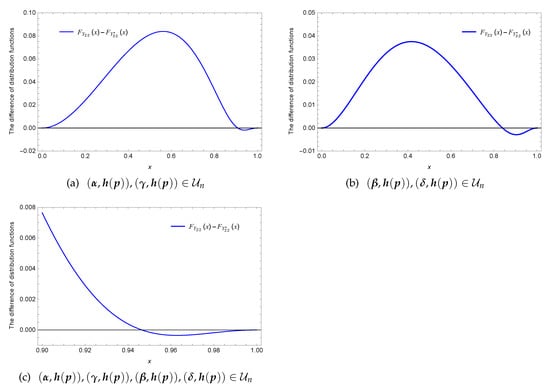
Let $X_i\sim MOTL-G({\alpha }_i,{\beta }_i,G\left(x\right))$ and $X_i^{*}\sim MOTL-G({\gamma }_i,{\delta }_i,G\left(x\right))$, $i=1,2$, assume that $I_{p_1},I_{p_2}$ be two independent Bernoulli random variables with $E\left(I_{p_i}\right)=p_i$, independent of $X_i\prime s(X_i^{*}\prime s)$, $i=1,2$. Let G(x)=x for $0\le x\le 1$, $h\left(p\right)=-log\left(p\right)$, and $(h\left(p_1\right),h\left(p_2\right))=(1,1.2)$.

(i) Let ${\beta }_1={\delta }_1=2$, ${\beta }_2={\delta }_2=5.5$, $({\alpha }_1,{\alpha }_2)=(1,8)$ and $({\gamma }_1,{\gamma }_2)=(4,6)$. Then, $(\mathbf{\alpha },\mathbf{h}\left(\mathbf{p}\right)),(\mathbf{\gamma },\mathbf{h}\left(\mathbf{p}\right))\in {\mathcal{U}}_n$ and $\mathbf{\alpha }\stackrel{\mathrm{w}}{⪰}\mathbf{\gamma }$. In this case, the distribution function $F_{Y_{2:2}}\left(x\right)-F_{Y_{2:2}^{*}}\left(x\right)$ is displayed in Figure 6a, which implies that the usual stochastic ordering does not hold between $Y_{2:2}$ and $Y_{2:2}^{*}$.

Figure 6. Plot of $F_{Y_{2:2}}\left(x\right)-F_{Y_{2:2}^{*}}\left(x\right)$.

(ii) Let ${\alpha }_1={\gamma }_1=1$, ${\alpha }_2={\gamma }_2=8$, $({\beta }_1,{\beta }_2)=(2,5.5)$ and $({\delta }_1,{\delta }_2)=(3,5)$. Then, $(\mathbf{\beta },\mathbf{h}\left(\mathbf{p}\right)),(\mathbf{\delta },\mathbf{h}\left(\mathbf{p}\right))\in {\mathcal{U}}_n$ and $\mathbf{\beta }\stackrel{\mathrm{w}}{⪰}\mathbf{\delta }$. However, Figure 6b shows that there exists no usual stochastic ordering between $Y_{2:2}$ and $Y_{2:2}^{*}$.

(iii) Let $({\alpha }_1,{\alpha }_2)=(1,8)$ and $({\gamma }_1,{\gamma }_2)=(4,6)$, $({\beta }_1,{\beta }_2)=(2,5.5)$ and $({\delta }_1,{\delta }_2)=(3,5)$. Then, $(\mathbf{\alpha },\mathbf{h}\left(\mathbf{p}\right)),(\mathbf{\gamma },\mathbf{h}\left(\mathbf{p}\right))\in {\mathcal{U}}_n$ and $(\mathbf{\beta },\mathbf{h}\left(\mathbf{p}\right)),(\mathbf{\delta },\mathbf{h}\left(\mathbf{p}\right))\in {\mathcal{U}}_n$, $\mathbf{\alpha }\stackrel{\mathrm{w}}{⪰}\mathbf{\gamma }$ and $\mathbf{\beta }\stackrel{\mathrm{w}}{⪰}\mathbf{\delta }$. However, Figure 6c shows that there exists no usual stochastic ordering between $Y_{2:2}$ and $Y_{2:2}^{*}$.

The following example is given to illustrate that the results of Theorem 8 cannot be strengthened from the usual stochastic order to reversed hazard rate order.

Example 8.

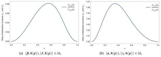
Under the same setup as part (i) of Example 7, we take ${\beta }_1={\beta }_2={\delta }_1={\delta }_2=2$ with the other conditions remaining unchanged. Similarly, in part (ii) of example 7, we take ${\alpha }_1={\alpha }_2={\gamma }_1={\gamma }_2=1$ with the other conditions remaining unchanged. Figure 7 shows that $F_{Y_{2:2}}\left(x\right)/F_{Y_{2:2}^{*}}\left(x\right)$ is not monotone in x. Therefore, neither $Y_{2:2}{\le }_{rh}{Y}_{2:2}^{*}$ of $Y_{2:2}{\ge }_{rh}{Y}_{2:2}^{*}$ is true.

Figure 7. The ratio of distribution functions $Y_{2:2}$ and $Y_{2:2}^{*}$.

4. Applications of the Real Data in the Series System Reliability

In this section, based on the real data, we apply the obtained results to analyze the reliability of the series system with dependent components.

In order to validate the effectiveness and practicability of the proposed methods in reliability engineering, we used the observed data of wind speeds from two wind farms, which are defined as site A and site B, respectively. Statistical characteristics of wind speed of two sites are shown in Table 1. Eryilmaz and kan [44] selected the Gumbel copula

$$C(u_1,u_2)=exp\{-{[{(-ln{u}_1)}^{\theta }+{(-ln{u}_2)}^{\theta }]}^{\frac{1}{\theta }}\},\theta \ge 1$$

to model the dependence structure of wind speeds at two sites, and Xie et al. [45] estimated the dependent parameter $\widehat{\theta }=3.32$ by a two-stage maximum likelihood estimation (MLE). Further, Eryilmaz and Kan [44] have assumed Rayleigh distribution

$$F\left(x\right)=1-e^{-\frac{x^2}{2b^2}},x\ge 0$$

for modeling the marginal wind speed distribution, and used the maximum likelihood estimator to obtain parameter ${\widehat{b}}_1=3.3662$ and ${\widehat{b}}_2=3.4271$ at site A and site B based on the real data, respectively. Now, just as Zhao et al. [46] discussed the reliability of a series system in shock environment, a reliability design engineer wants to assess the effects of model parameters on the reliability of a two-rolling bearing systems of a wind turbine. As it is difficult to collect data of surviving probabilities after the system subject to random shock, so we assume that this random shock have no impact on the lifetime of component, that is, the probability of component survival are $\mathit{p}={\mathit{p}}^{*}=(1,1,1)$. Further, we choose the Rayleigh distribution as the baseline distribution, and set the vectors of shape parameters ${\mathbf{\alpha }}_1=(0.2,2.6,5.4)$, ${\mathbf{\alpha }}_2=(0.85,2.6,5.1)$ and ${\mathbf{\alpha }}_3=(2.96,2.96,2.96)$. Based on the real data and Theorem 2, the reliability of series system ($Y_{1:3}$) can be expressed by

$$\begin{array}{ccc}\hfill {\overline{F}}_{Y_{1:3}}\left(x\right)& =& \prod _{i=1}^3{p}_i\psi \left(\sum _{i=1}^3\varphi \left(\zeta ({\alpha }_i,2,1-e^{-\frac{x^2}{2b_1^2}})\right)\right)\hfill \\ & =& exp\{-{[{(-{lnc}_1)}^{3.32}+{(-{lnc}_2)}^{3.32}+{(-{lnc}_3)}^{3.32}]}^{\frac{1}{3.32}}\},\hfill \end{array}$$

where $c_i=\frac{{\alpha }_i\left(1-{\left(1-{\left(1-G_1\left(x\right)\right)}^2\right)}^2\right)}{{\alpha }_i+{\overline{\alpha }}_i{\left(1-{\left(1-G_1\left(x\right)\right)}^2\right)}^2}$, $G_1\left(x\right)=1-e^{-\frac{x^2}{2b_1^2}}$, and $i=1,2,3$, and we give the curves of the reliability function under the different parameters vectors as shown in Figure 8. Figure 8 indicates that the weaker heterogeneity among shape parameters according to the weak majorization order leads to larger reliability of the series systems. Therefore, a reliability design engineer can use the results to assess the reliability performance or increase the availability of a series system with dependent components.

Table 1. Statistical characteristics of wind speed data from two sites.

Statistics	Eidhoven (Site A)	Volkel (Site B)
Mean	4.25	4.14
Standard	2.33	2.35

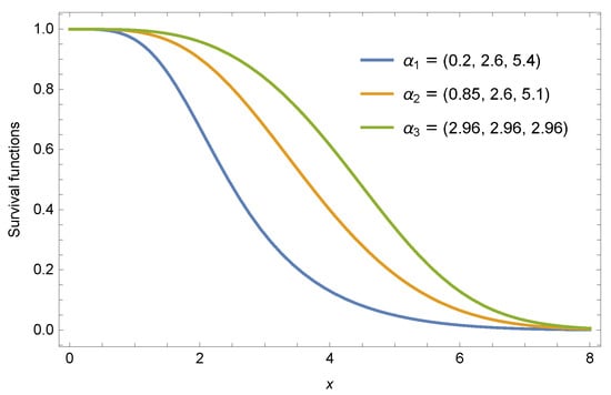
Figure 8. Curves of the reliability functions of a series system.

5. Analysis of the Obtained Results

To compare the results of the experiment with the obtained theoretical data, we use the Clayton copula

$$C(u_1,u_2)={\left[max(u_1^{\theta }+u_2^{\theta }-1,0)\right]}^{-\frac{1}{\theta }},\theta \ge 0$$

and Rayleigh distribution conducting experiment analysis, where Wang and Li [47] estimated the Clayton copula parameters $\widehat{\theta }=0.6474$ and Eryilmae and kan [44] used the maximum likelihood estimator to obtain Rayleigh distribution parameter ${\widehat{b}}_1=3.3662$ and ${\widehat{b}}_2=3.4271$ by real data. Based on the obtained theoretical data of Example 1 and the estimator value of parameters, we plot the curves of reliability functions of under the different parameters as shown in Figure 9. First, we can see from the graph that two curves do not intersect each other, which means that the theoretical approach is feasible. Second, for different shape and copula parameters, the more positive dependence, the weaker heterogeneity among shape parameters according to the row weak majorization order leads to larger reliability of the series system. Therefore, we can conclude that the influence of the results of the experiment and obtained theoretical data on the reliabilities of series system is consistent as Remark 3, so we may be think that the theoretical characteristics of the research can be used as the evaluation of system performance in reliability engineering.

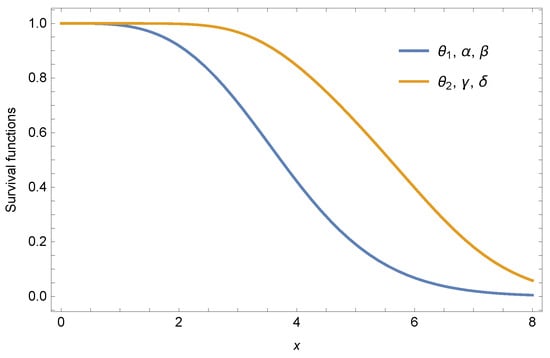
Figure 9. Curves of the survival functions of $Y_{1:3}$ and $Y_{1:3}^{*}$.

6. Conclusions

In the last section, we provide the innovation, the scientific and practical conclusions and future topic of this manuscript.

6.1. Innovation of Research

Stochastic comparison of system lifetimes has always been an important research topic in reliability optimization and survival analysis. Many works have also been discussed in the past years to compare the lifetimes of the system with heterogeneous independent components. However, in practical situations, the components’ lifetimes may be dependent because the components of the system are influenced by common environment, workload, and stress. In addition, the system is often confronted with random shocks from an external stressing environment, as well as competing soft and sudden failures, and the random shocks may result in component failure and affect system reliability. In this sense, this paper carries out work from two aspects: on the one hand, it considers the dependence between components, and on the other hand, it also considers the influence of random shock on system reliability.

6.2. Scientific and Practical Conclusions

In this paper, we study the effect heterogeneity of among shape parameters and surviving probabilities from random shocks on the reliability of systems with dependent or independent heterogeneous MOTL-G components subject to random shocks. The detailed information about main results can be summarized as follows.

First, we obtain the usual stochastic and hazard rate orders between two series systems comprising dependent heterogeneous components under random shocks. Second, a comparison result is obtained for parallel systems from two heterogeneous dependent components in the sense of usual stochastic order between the transformations of surviving probabilities $\mathit{h}\left(\mathit{p}\right)$ and $\mathit{h}\left({\mathit{p}}^{*}\right)$ from random shocks. Finally, we consider the usual stochastic order for parallel systems with independent heterogeneous components subject to random shocks. Moreover, it is demonstrated through Example 8 that the result of Theorem 8 cannot be strengthened from the usual stochastic order to reversed hazard rate order.

The results show that the weaker heterogeneity between shape parameters $\mathbf{\alpha }$ ($\mathbf{\beta }$) and $\mathbf{\gamma }$ ($\mathbf{\delta }$), according to the weaker majorization order, results in larger reliability of series and parallel systems, and indicates that the more heterogeneity of the transformations of surviving probabilities $\mathit{h}\left(\mathit{p}\right)$ and $\mathit{h}\left({\mathit{p}}^{*}\right)$ under random shocks in terms of the weaker majorization order leads to better parallel system reliability. The results of this paper can be also applied to a wide variety of distributions generated from MOTL distribution through specified baseline distributed function G as discussed in the Introduction. These ordering properties can be used to select the best system structure under different configuration or to investigate where to put the different components in a system structure, and their properties are rather useful in other areas such as operations research, insurance and survival analysis, etc.

6.3. Future Topic

In the present work, we only provide sufficient conditions for comparison of the lifetimes of the series and parallel systems with dependent heterogeneous MOTL-G components under random shocks. Nevertheless, many systems are often composed of series-parallel, parallel-series, and coherent systems in reliability engineering. The main limitation of the proposed new model is the lack of reliability analysis of these systems, which have a more complex system structure that causes great challenges. Meanwhile, the dependent structure of components is only coupled by Archimedean Copula, but in actual engineering, the interdependence between components may be Farlie–Gumbel–Morgenstern (FGM) copula. Accordingly, the FGM copula can be used to characterize the interdependence between components in future research. Besides, we assume that all surviving probabilities from random shocks are mutually independent. However, in most practical scenarios of reliability engineering, the lifetime of component and surviving probabilities may be dependent as they usually work in the same environment. These interesting problems remain open and merit further discussion.

References

- Zhao, P.; Balakrishnan, N. New results on comparisons of parallel systems with heterogeneous gamma components. Stat. Probab. Lett. 2011, 81, 36–44. [Google Scholar] [CrossRef]
- Yan, R.; Da, G.; Zhao, P. Further results for parallel systems with two heterogeneous exponential components. Statistics 2013, 47, 1128–1140. [Google Scholar] [CrossRef]
- Zhao, P. On parallel systems with heterogeneous gamma components. Probab. Eng. Inf. Sci. 2011, 25, 369–391. [Google Scholar] [CrossRef]
- Ding, W.; Yang, J.; Ling, X. On the skewness of extreme order statistics from heterogeneous samples. Commun. Stat.-Theory Methods 2017, 46, 2315–2331. [Google Scholar] [CrossRef]
- Balakrishnan, N.; Zhao, P. Ordering properties of order statistics from heterogeneous populations: A review with an emphasis on some recent developments. Probab. Eng. Inf. Sci. 2013, 27, 403–443. [Google Scholar] [CrossRef]
- Yan, R.; Wang, J. Component level versus system level at active redundancies for coherent systems with dependent heterogeneous components. Commun. Stat.-Theory Methods 2020, 1–21. [Google Scholar] [CrossRef]
- Yan, R.; Zhang, J.; Zhang, Y. Optimal Allocation of Relevations in coherent systems. J. Appl. Probab. 2021, 58, 1–22. [Google Scholar] [CrossRef]
- Zhang, J.; Yan, R. Stochastic comparison at component level and system level series system with two proportional hazards rate components. J. Quant. Econ. 2018, 35, 91–95. [Google Scholar]
- Kochar, S.C.; Torrado, N. On stochastic comparisons of largest order statistics in the scale model. Commun. Stat.-Theory Methods 2015, 44, 4132–4143. [Google Scholar] [CrossRef][Green Version]
- Fang, L.; Zhang, X. Stochastic comparisons of series systems with heterogeneous Weibull components. Stat. Probab. Lett. 2013, 83, 1649–1653. [Google Scholar] [CrossRef]
- Zhang, T.; Zhang, Y.; Zhao, P. Comparisons on largest order statistics from heterogeneous Gamma samples. Probab. Eng. Inf. Sci. 2021, 35, 611–630. [Google Scholar] [CrossRef]
- Zhang, Y.; Cai, X.; Zhao, P.; Wang, H. Stochastic comparisons of parallel and series systems with heterogeneous resilience-scaled components. Statistics 2019, 53, 126–147. [Google Scholar] [CrossRef]
- Fang, R.; Wang, B. Stochastic comparisons on sample extremes from independent or dependent gamma samples. Statistics 2020, 54, 841–855. [Google Scholar] [CrossRef]
- Zhao, P.; Li, X.; Balakrishnan, N. Likelihood ratio order of the second order statistic from independent heterogeneous exponential random variables. J. Multivar. Anal. 2009, 100, 952–962. [Google Scholar] [CrossRef][Green Version]
- Mercier, S.; Pham, H.H. A random shock model with mixed effect, including competing soft and sudden failures, and dependence. Methodol. Comput. Appl. Probab. 2016, 18, 377–400. [Google Scholar] [CrossRef]
- Kundu, A.; Chowdhury, S. Ordering properties of the largest order statistics from Kumaraswamy-G models under random shocks. Commun. Stat.-Theory Methods 2021, 50, 1502–1514. [Google Scholar] [CrossRef]
- Kundu, A.; Chowdhury, S.; Balakrishnan, N. Ordering properties of the smallest and largest lifetimes in Gompertz–Makeham model. Commun. Stat.-Theory Methods 2021, 1–30. [Google Scholar] [CrossRef]
- Fang, L.; Balakrishnan, N. Ordering properties of the smallest order statistics from generalized Birnbaum–Saunders models with associated random shocks. Metrika 2018, 81, 19–35. [Google Scholar] [CrossRef]
- Zhang, Y.; Amini-Seresht, E.; Zhao, P. On fail-safe systems under random shocks. Appl. Stoch. Model. Bus. Ind. 2019, 35, 591–602. [Google Scholar] [CrossRef]
- Das, S.; Kayal, S.; Balakrishnan, N. Orderings of the smallest claim amounts from exponentiated location-scale models. Methodol. Comput. Appl. Probab. 2021, 23, 971–999. [Google Scholar] [CrossRef]
- Nadeb, H.; Torabi, H.; Dolati, A. Stochastic comparisons between the extreme claim amounts from two heterogeneous portfolios in the case of transmuted-G model. N. Am. Actuar. J. 2020, 24, 475–487. [Google Scholar] [CrossRef]
- Balakrishnan, N.; Zhang, Y.; Zhao, P. Ordering the largest claim amounts and ranges from two sets of heterogeneous portfolios. Scand. Actuar. J. 2018, 1, 23–41. [Google Scholar] [CrossRef]
- Li, X.; Zuo, M.J. Preservation of stochastic orders for random minima and maxima, with applications. Nav. Res. Logist. 2004, 51, 332–344. [Google Scholar] [CrossRef]
- Hazra, N.K.; Nanda, A.K.; Shaked, M. Some aging properties of parallel and series systems with a random number of components. Nav. Res. Logist. 2014, 61, 238–243. [Google Scholar] [CrossRef]
- Barmalzan, G.; Najafabadi, A.T.P. On the convex transform and right-spread orders of smallest claim amounts. Insur. Math. Econ. 2015, 64, 380–384. [Google Scholar] [CrossRef]
- Barmalzan, G.; Najafabadi, A.T.P.; Balakrishnan, N. Likelihood ratio and dispersive orders for smallest order statistics and smallest claim amounts from heterogeneous Weibull sample. Stat. Probab. Lett. 2016, 110, 1–7. [Google Scholar] [CrossRef]
- Zhang, Y.; Zhao, P. Comparisons on aggregate risks from two sets of heterogeneous portfolios. Insur. Math. Econ. 2015, 65, 124–135. [Google Scholar] [CrossRef]
- Li, C.; Li, X. Stochastic comparisons of parallel and series systems of dependent components equipped with starting devices. Commun. Stat.-Theory Methods 2019, 48, 694–708. [Google Scholar] [CrossRef]
- Panja, A.; Kundu, P.; Pradhan, B. Stochastic comparisons of lifetimes of series and parallel systems with dependent and heterogeneous components. Oper. Res. Lett. 2021, 49, 176–183. [Google Scholar] [CrossRef]
- Zhang, J.; Yan, R.; Wang, J. Reliability of parallel-series and series-parallel systems with statistically dependent components. Appl. Math. Model. 2021, 102, 618–639. [Google Scholar] [CrossRef]
- Zhang, M.; Lu, B.; Yan, R. Ordering results of extreme order statistics from dependent and heterogeneous modified proportional (reversed) hazard variables. AIMS Math. 2021, 6, 584–606. [Google Scholar] [CrossRef]
- Guo, Z.; Zhang, J.; Yan, R. On inactivity times of failed components of coherent system under double monitoring. Probab. Eng. Inf. Sci. 2021, 1–18. [Google Scholar] [CrossRef]
- Yan, R.; Wang, J.; Lu, B. Orderings of component level versus system level at active redundancies for coherent systems with dependent components. Probab. Eng. Inf. Sci. 2021, 1–23. [Google Scholar] [CrossRef]
- Marshall, A.W.; Olkin, I. A new method for adding a parameter to a family of distributions with application to the exponential and Weibull families. Biometrika 1997, 84, 641–652. [Google Scholar] [CrossRef]
- Al-Shomrani, A.; Arif, O.; Shawky, A.; Hanif, S.; Shahbaz, M.Q. Topp–Leone family of distributions: Some properties and application. Pak. J. Stat. Oper. Res. 2016, 12, 443–451. [Google Scholar] [CrossRef]
- Khaleel, M.A.; Oguntunde, P.E.; Al Abbasi, J.N.; Ibrahim, N.A.; AbuJarad, M.H. The Marshall-Olkin Topp Leone-G family of distributions: A family for generalizing probability models. Sci. Afr. 2020, 8, 1–19. [Google Scholar] [CrossRef]
- Muirhead, R.F. Some methods applicable to identities and inequalities of symmetric algebraic functions of n letters. Proc. Edinb. Math. Soc. 1902, 21, 144–162. [Google Scholar] [CrossRef]
- Marshall, A.W.; Olkin, I.; Arnold, B.C. Inequalities: Theory of Majorization and Its Applications; Springer: New York, NY, USA, 2011. [Google Scholar]
- Kleinbaum, D.G.; Klein, M. Survival Analysis; Springer: New York, NY, USA, 2010. [Google Scholar]
- Shaked, M.; Shanthikumar, J.G. Stochastic Orders; Springer: New York, NY, USA, 2007. [Google Scholar]
- Nelsen, R.B. An Introduction to Copulas; Springer: New York, NY, USA, 2006. [Google Scholar]
- Fang, R.; Li, C.; Li, X. Stochastic comparisons on sample extremes of dependent and heterogenous observations. Statistics 2016, 50, 930–955. [Google Scholar] [CrossRef]
- Zhang, L.; Yan, R. Stochastic comparisons of series and parallel systems with dependent and heterogeneous Topp-Leone generated components. AIMS Math. 2021, 6, 2031–2047. [Google Scholar] [CrossRef]
- Eryilmaz, S.; Kan, C. Reliability based modeling and analysis for a wind power system integrated by two wind farms considering wind speed dependence. Reliab. Eng. Syst. Saf. 2020, 203, 107077. [Google Scholar] [CrossRef]
- Xie, K.; Li, Y.; Li, W. Modelling wind speed dependence in system reliability assessment using copulas. IET Renew. Power Gener. 2012, 6, 392–399. [Google Scholar] [CrossRef]
- Zhao, X.; Lv, Z.; He, Z.; Wang, W. Reliability and opportunistic maintenance for a series system with multi-stage accelerated damage in shock environments. Comput. Ind. Eng. 2019, 137, 106029. [Google Scholar] [CrossRef]
- Wang, F.; Li, H. Distribution modeling for reliability analysis: Impact of multiple dependences and probability model selection. Appl. Math. Model. 2018, 59, 483–499. [Google Scholar] [CrossRef]
Publisher’s Note: MDPI stays neutral with regard to jurisdictional claims in published maps and institutional affiliations. |
© 2021 by the authors. Licensee MDPI, Basel, Switzerland. This article is an open access article distributed under the terms and conditions of the Creative Commons Attribution (CC BY) license (https://creativecommons.org/licenses/by/4.0/).