Abstract
There are a variety of degradation models in the literature, each with a certain effect of random variation around the mean degradation path on the time-to-failure of the device being degraded. To assess the dependence that the random variation around the mean degradation path exerts on the resulting time-to-failure, this paper presents copula functions for time-to-failure-based degradation models with respect to two well-known degradation models, namely, the multiplicative degradation model and the additive degradation model. The implied copula functions for the case of the multiplicative degradation model have explicit forms. The implied copula functions are proved to be symmetric in the case of deterministic effect of degradation on failure, but the copulas obtained when failure is affected uncertainly by degradation are asymmetric. Necessary and sufficient conditions for the implicit copula functions to be symmetric are given.
1. Introduction
In general, copulas are multivariate functions and, in a special case, bivariate functions that are useful to describe the dependence structure of multivariate and bivariate distributions, regardless of what the marginal distributions of the underlying multivariate and bivariate distributions are. More precisely, copulas allow the separation of the dependence effect from the effects of the marginal distributions. Nelsen [1] provides a set of methods for constructing bivariate distributions over bivariate copulas. For the study of dependence in some bivariate families, we refer to Genest [2], Joe [3], Nadarajah et al. [4], Durante [5], and Tang et al. [6], among others. We now begin with the definition of copula, our preliminary work, and auxiliary results.
A bivariate function is a copula if it satisfies the following conditions:
1. Boundary condition, For and
2. Increasing property. For all and
Sklar’s theorem states that if is a bivariate df. and and are its marginal distributions, then there is a unique copula such that
If C is a copula and and are univariate continuous distributions, then (1) defines a bivariate distribution with marginal cumulative distribution functions (c.d.f.s) and . Let , and denote the survival functions (s.f.s) of , X and Y, respectively. The previous formula leads to
The function is called the survival copula, which is linked to C via the next formula
Notice that C and coincide with independent copula when X and Y are independent, that is,
It is well known that for any copula C and for all ,
where . Note that previous bivariate functions and are themselves copulas called Fréchet–Hoeffding bounds. More information about the construction of these bounds is presented in Fréchet [7]. For more details on the notion of copulas, we refer the interested reader to Nelsen [1]. One of the attractive properties of copulas is symmetry. A bivariate copula function C is said to be symmetric if for all (see, e.g., Genest et al. [8]). The copulas W and M are both symmetric copulas.
In many cases, it may be difficult to measure or maintain the lifetime of a particular item because of longevity and/or failures caused by unexpected cumulative random shocks. In such situations, if a cumulative degradation feature related to lifetime can be observed, then the reliability or percentile of lifetime can be modeled using these degradation measurements. Degradation modeling has been an effective reliability analysis approach for products with failures caused by degradation. Stochastic degradation process models are developed on the basis of cumulative degradation signals of systems under three types of thresholds: namely, alarm line and two different failure thresholds. One of the failure thresholds is the degradation amount, and the other corresponds to the duration. Degradation models are mainly classified into three classes: namely, stochastic process models, general path models, and other models beyond the both (cf. Ye and Xie [9]). In recent years, the analysis of degradation data has played an important role in various disciplines such as reliability, health sciences, and finance. For example, by analyzing degradation data, information can be obtained about the reliability of a highly reliable product. Statistical modeling and inference techniques have been developed based on various degradation measures. Degradation data can provide much more information than failure data because they provide more information about product life status than failure data if a specific degradation mechanism can be identified. Modeling and analysis with the degradation signal is useful in predicting product life. Systems used in the production of goods and the delivery of services comprise the majority of capital in most industries. These systems are subject to degradation with use and age (see, e.g., Valdez-Flores and Feldman [10]). We review methods developed in the field of degradation-based modeling that are considered indispensable and operational for making inferences about the lifetimes of various types of deteriorating systems (see, e.g., Kharoufeh and Cox [11], Park and Padgett [12], Gebraeel and Pan [13], Kharoufeh et al. [14], Jiang et al. [15], Peng and Tseng [16], Ye and Xie [9], Chen et al. [17], Chen and Ye [18], Bressi et al. [19], and He [20]). The lifetime of deteriorating items that exhibit observable deterioration can generally be modeled by a stochastic process, particularly an inhomogeneous gamma process or an inhomogeneous inverse Gaussian process. For example, a measurement error with respect to a device that increases with time can be accounted for. For systems with high reliability, strategies based on degradation data may be the only possible framework to achieve the goal of reliability analysis. Therefore, the methods developed for degradation data analysis have become typical tools in the last decades. The analysis of degradation data is possible after the definition of lifetime has been established (see, e.g., Liu et al. [21]).
As stated by Bae et al. [22], most practical degradation strategies satisfy two degradation models, namely the multiplicative degradation model and the additive degradation model. In these models, there is a mean degradation path and also a random factor X, which is called random variation around the mean degradation path. By applying a deterministic criterion for the failure of a device subject to degradation, implicit distributions of lifetime are obtained. Recently, Albabtain et al. [23] developed a modified dynamic criterion for the failure of a device under degradation. Denote by T the resulting lifetime variable in each case. Bae et al. [22] studied the effect of stochastic changes with respect to X on the stochastic variation of T based on different stochastic orders. Kayid and Alshagrawi [24] applied degradation models with multiplicative and additive paths in the model developed by Albabtain et al. [23], where a modified dynamic degradation-based time-to-failure model has been introduced. They investigated the preservation of stochastic orders on X to be preserved by T. To have a critical perspective on the foregoing literature, it can be realized that most of the works that consider connections between X and T study only how they are connected, and the question of why they are connected has not been addressed anywhere. Continuing to look for a broader source of creation of the state or the extent to which X and T are being connected remains as an unanswered problem. This paper aims to find the copula function of the random pair in different degradation models which is considered to be the source of connection of X and T.
That a stochastic change in random variation X, which is a main component in degradation models with a multiplicative path and also degradation models with an additive path, leads to a same stochastic change in the resulting lifetime T may be an indication that X and T are statistically dependent. Therefore, the dependence structure induced by the pair is worth considering. Izadkhah et al. [25] demonstrated that some partial dependencies between X and T are characterized by stochastic order relations between the conditional distribution of T at certain levels of X. However, to analyze the dependency in a more complete framework not in a partial way, the joint distribution function of T and X, if it can be obtained, may be used to identify the entire aspects of dependency between T and X. Following the studies accomplished by Bae et al. [22] and Kayid and Alshagrawi [24], it is realized that the influence of X on T is significant, which in turn motivates us to consider the dependencies between X and T in multiple degradation models as a meaningful problem. In this paper, we apply the notion of copula function in the described context to present a mechanism for evaluating the dependence between the random variation X and the resulting lifetime variable T in multiplicative degradation model and also additive degradation model.
The paper is organized as follows. In Section 2, for time-to-failure models arising from a set of degradation models in which an increasing (or decreasing) degree of degradation is the only reason for failure, we characterize the copula functions of the implied lifetime and random variation components in the degradation models. The implied copula functions are known to be reputable in the literature. In Section 3, the two degradation models are placed in the framework of the dynamic time-to-failure model proposed by Albabtain et al. [23] to derive the implied copula function between the implied lifetime and random variation components. The curves of the copulas are plotted along with the corresponding contour plots. Section 4 concludes the paper with further intuitive remarks on the current work and also contains some statements for future work.
2. Models with Deterministic Degradation Effect on Failure
For highly reliable products, the criterion for classifying a device as a failed device is described in terms of the first passage time of a stochastic process. More specifically, if stochastic processes with monotonic sampling paths are considered, then the traditional definition of a degradation model assumes that the failure of an item/system occurs when the degradation exceeds the given threshold . Assume that failure is modeled by a stochastic process that maintains monotonically increasing pattern paths, as is common in many practical situations. Let the time to failure be denoted by the random variable T. According to the described failure criterion, T is the time of the first pass to threshold , given by . The corresponding distribution function of failures is denoted by , and the implied survival function is denoted by . The monotonicity of a realization of the stochastic process ensures with probability one that for . Therefore,
As Bae et al. (2007) point out, in most practical applications, the degradation functions go beyond the elementary functions listed in their work, including an additive degradation model and a multiplicative degradation model as two frequently used degradation models. The general multiplicative degradation model is given as follows.
where is the mean degradation path. The mean degradation path is considered to be a monotonically increasing function. Let denote the s.f. of lifetime T under the multiplicative degradation model (2). Since , the usual first passage time criterion yields .
The general additive degradation model is given as follows.
where is a deterministic mean degradation path for time Since the mean degradation path is usually a monotonic function, only the cases where is monotonic are considered. The random variable X represents the random variation around the deterministic mean degradation path with c.d.f. and probability density function (p.d.f.) . Denote by the s.f. of the lifetime T under the additive degradation model (3). Using the criterion for device failure under degradation and relying on , we then conclude that .
To determine the influence of the random variation X on the lifetime T in a degradation model, the copula functions between X (random variation) and T (the resulting lifetime) can be captured, through which various stochastic dependence properties between T and X are realized.
If T is the lifetime, then models (2) and (3), respectively, define the transformation to (see, e.g., Bae et al. [22]). The conservation properties of aging terms and stochastic orderings on X for lifetime T have been studied by some researchers (see e.g., Bae et al. [22] and Li et al. [26]). In the multiplicative degradation model, consider the conditional probability as the amount SF of T at calculated by
where is the indicator of the set A. Evidently, is the associated conditional c.d.f. To obtain the bivariate c.d.f. of we have
Following that concluded from (2), we have , and thus, for all ,
Hence, by Sklar’s theorem, the copula function associated with the couple is
which is the lower bound of Fréchet–Hoeffding for the copulas given in (3). This emphasizes that X has the hardest possible negative effect on T, so the dependency is severely negative.
In the additive degradation model, let us derive the conditional probability as the value of SF of T given obtained by
For the associated conditional c.d.f., one gets . The bivariate c.d.f. of is grasped as
Following the conclusion of (3), one has and, as a result, for all ,
Therefore, by Sklar’s theorem, the copula function of is acquired as
which is again the lower bound of Fréchet–Hoeffding for copulas, and this is a sign that X has the severest possible negative effect on the lifetime T. The implied copula function is , which is a symmetric copula.
3. Models with Uncertain Degradation Effect on Failure
Albabtain et al. [23] initiated a new methodology for modeling time-to-failure data based on degradation processes. They considered it controversial to consider a predetermined threshold as the cutoff value for the degree of degradation that causes an item to fail. They established a modified criterion for the failure of an item under degradation that satisfies many situations to increase the risks of hard failure and also soft failure for the item under consideration. From the definition of T in the traditional method, the only reason for the failure of the system is a degradation increase up to a certain level such that and . However, this property applies to systems with high reliability that can be assigned a stepwise failure. Consideration of such a fixed threshold may not be appropriate in realistic situations. It is better to consider the possibility of sudden failure, since the link between the time to failure and the degradation process may not be deterministic to obtain the s.f. of T as usual. Albabtain et al. [23] have proposed a dynamic degradation-based time-to-failure model in which as a probability measure adjusts the failure probabilities at different degradation levels.
The amount of degradation at time t is denoted by following p.d.f. and the c.d.f. According to the dynamic model of Albabtain et al. [23], the time-to-failure T that follows the implied lifetime distribution under the degradation process has the s.f.
where is a conditional limiting probability given by
Kayid and Alshagrawi [24] developed the model (7) under both the additive degradation model and the multiplicative degradation model. Let X follow p.d.f. and c.d.f. . In this regard, when a multiplicative degradation model is under consideration, then they deduced that (7) leads to
in which
Therefore,
It is deduced that For the additive degradation model, Kayid and Alshagrawi [24] established that (7) leads to
in which the expectation is with respect to X. By considering the additive degradation model (3), we get
where is the joint s.f. of T and X. We can write
in which is the conditional s.f. of T given . Therefore,
In the rest of the paper, the copulas resulting from the model (5) and the model (6) for will be characterized. First, we present general formulas for the copula functions associated with .
In the context of the model (8) where for all , the implied lifetime distribution has s.f. . Denote by the conditional s.f. of T given and also denote by the indicator function of the set A. To derive the joint c.d.f. of we can write
The associated joint p.d.f., whenever is absolutely continuous, is given by
In parallel, the model (9) when it applied where for all is considered, then the implied lifetime distribution has s.f. . The joint c.d.f. of can be obtained in this case as
If in (11) is absolutely continuous, then the joint density of is derived as
In a more general setting, when the degradation satisfies other forms, T and X have a joint c.d.f.
Provided that in (12) is absolutely continuous, the associated joint p.d.f. is obtained as
By Sklar’s theorem, we develop the copula formula in terms of (12) as will be followed from which copula functions in both multiplicative and additive models, respectively, when and can be built:
On the other hand, for all if, and only if,
Therefore, Equation (13) concludes that
We present some necessary and sufficient conditions under which the copula function (13) or equivalently (14) is symmetric. Suppose that
Theorem 1.
Let there exist functions and on such that Then, the implied copula function (14) is symmetric, if and only if for all
Proof.
Note that the copula function (13) satisfies for all and thus, it is symmetric if, and only if for all ,
which is equivalent to saying that for all ,
This holds by assumption if, and only if,
in which Y is a uniform random variable on . It is straightforward that if for all , then C is symmetric. Conversely, since the family of uniform distribution on where is a complete family of distributions, thus, it is concluded that for all . The proof is completed. □
The copula function (14) can be developed for the cases where is partially or fully specified. In this paper, we consider the cases where for all , and , assuming is stochastically increasing and for all , and in situations where is stochastically decreasing. To apply these conditions to the particular cases of the additive degradation model and the multiplicative degradation model, the function is considered to be increasing and decreasing in t, respectively.
The following part of the paper contributes to characterizing the copula function in some routine degradation-based time-to-failure models in the special cases of additive and multiplicative degradation paths. As a fundamental property, the method is applied to extract the exact forms of copula function in some respected time-to-failure models. From another perspective, it has been shown that in a degradation-based time-to-failure model, where the random variation around the mean degradation path is the underlying independent variable, the copula function of the random variation around the mean degradation path as the independent variable and the implied lifetime as the dependent variable can be accurately determined in multiplicative degradation models, and thus, the shape of the copula function in this case is free of the mean degradation path and is also independent of the survival probability at certain levels of w. Thus, the explicit copula functions that we will derive are owed to the multiplicative degradation model.
Systems with multiple components exhibit some degree of dependence between the performances of their components, which are realized through some connections between the lifetimes of the components. This dependence can be positive, for example, when the time to failure of the components is subject to a common environment. Negative dependencies arise, for example, in competing risk models where components compete for a fixed number of resources. The statistical literature contains many references to various measures of dependence, including the correlation and partial correlation coefficients. The notion of association between random variables has many applications in reliability and other life sciences.
Several copula functions are generated under four time-to-failure degradation models, each of which evolves beyond a particular property of when w is a realization of either the multiplicative model or the additive model
Assume that , where the mean degradation path function is an increasing function. Assume that is a decreasing function. We consider the model
where indicates that is the probability of survival until time t at which the degradation is valued to be one unit. It is notable from (15) that and for all . The implied lifetime distribution under (15) when X has exponential distribution with mean has s.f.
Note that the construction of copula functions is independent of the choice of marginal distributions. Let us assume that X has an arbitrary c.d.f. . Then, by total probability, formula T follows the c.d.f. given by
where follows the uniform distribution on for every arbitrary choice of . It is trivial that the probability does not depend on because the influences of this distribution have been fixed to the uniform distribution, and thus, the derivation of is not affected by the choice of but only the copula function of T and X. Notice that which makes copula as an independent identity of bivariate distribution of apart from the marginal distributions and . Thus, from (10), if we take X as a random variable with exponential distribution with mean having c.d.f. , then
By using (16), the bivariate c.d.f. of in (17) is modified as
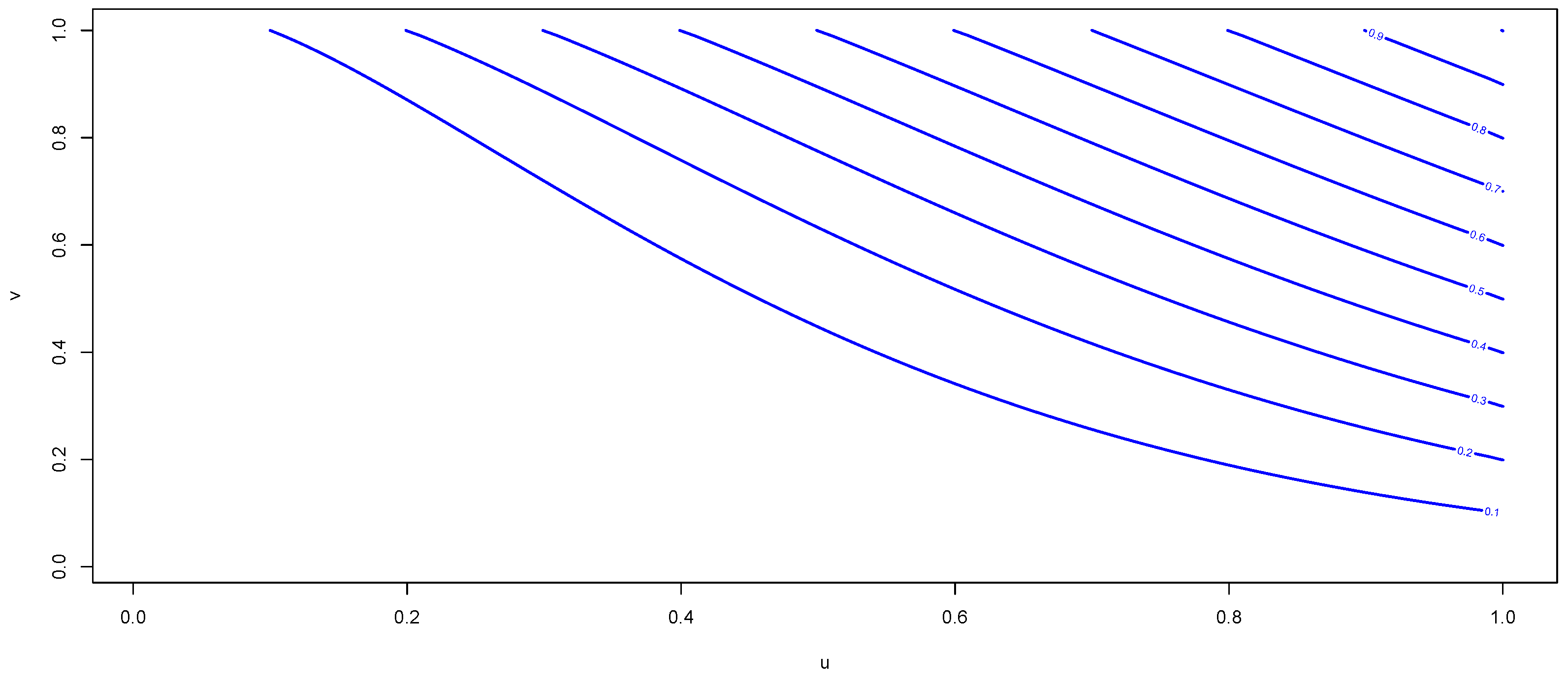
Therefore, the copula function is obtained by (18) and applying Sklar’s theorem as follows:
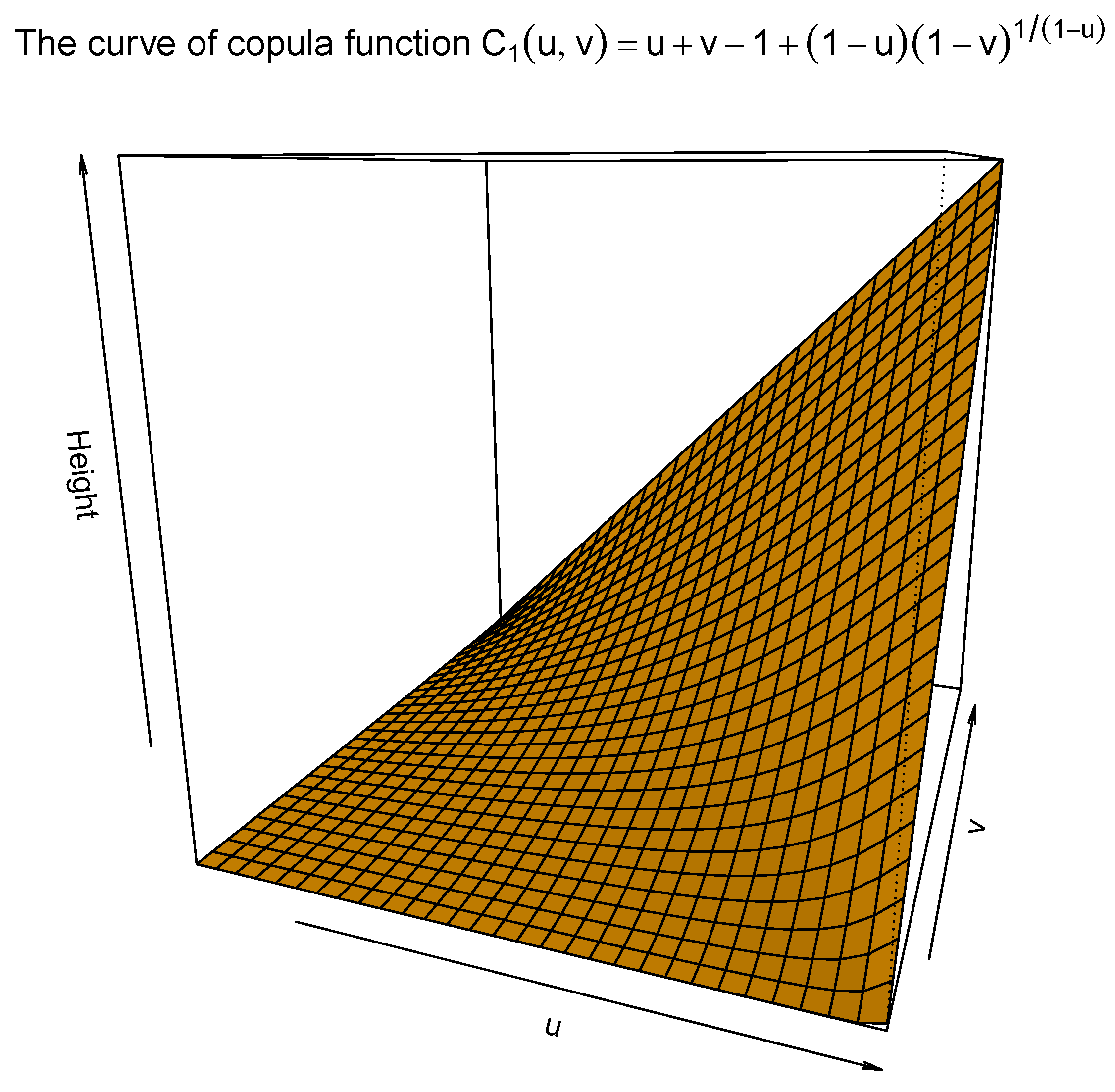
The curve of the copula function in (19) is plotted in Figure 1, and also, the contour lines associated with this copula function are drawn in Figure 2.

Figure 1.
The curve of the implied copula function .
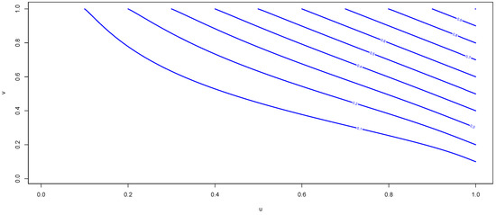
Figure 2.
Copula contour plot of .
We now suppose that in which the mean degradation path function is increasing. Let be a decreasing function. The probability for survival until time t at degradation level is considered as
Note that and denote . It is once again obvious from (20) that and for all . The implied lifetime distribution after imposing (20) with X following inverse Weibull distribution with c.d.f. where has s.f.
In the spirit of (10), if X follows the c.d.f. , then
By applying (21), the c.d.f. of in (22) can be rewritten as
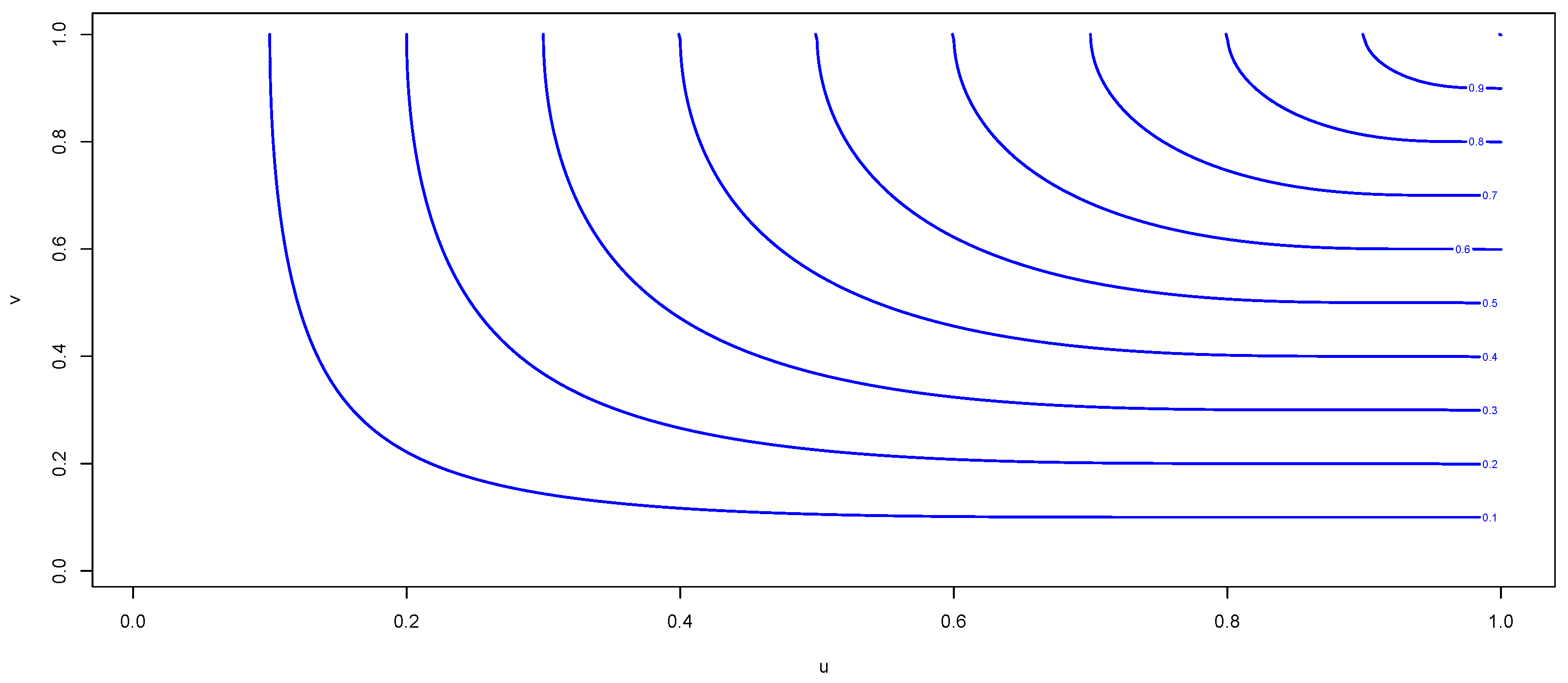
Then, the associated copula function is obtained from (23) when Sklar’s theorem is applied. We have
The plot of the copula function in (24) is drawn in Figure 3, and the contour lines for this copula function are plotted in Figure 4.
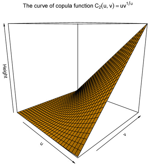
Figure 3.
The curve of the implied copula function .
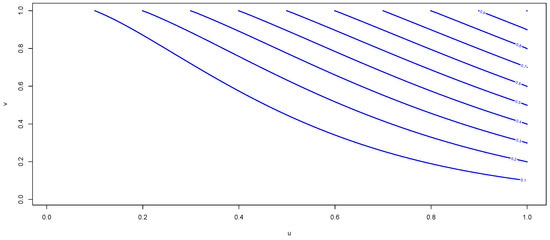
Figure 4.
Copula contour plot of .
Let us now consider multiplicative degradation models with a decreasing mean degradation path. Suppose that , where is a decreasing function. The function is considered to be decreasing. We assume that
Note that . To examine the limits of at endpoints of degradation levels from (25), we realize that and for all . By (25), the implied lifetime distribution with a random variable X from inverse Weibull distribution with c.d.f. in which is proved to have s.f.
Using (26), the c.d.f. of in (27) is obtained as
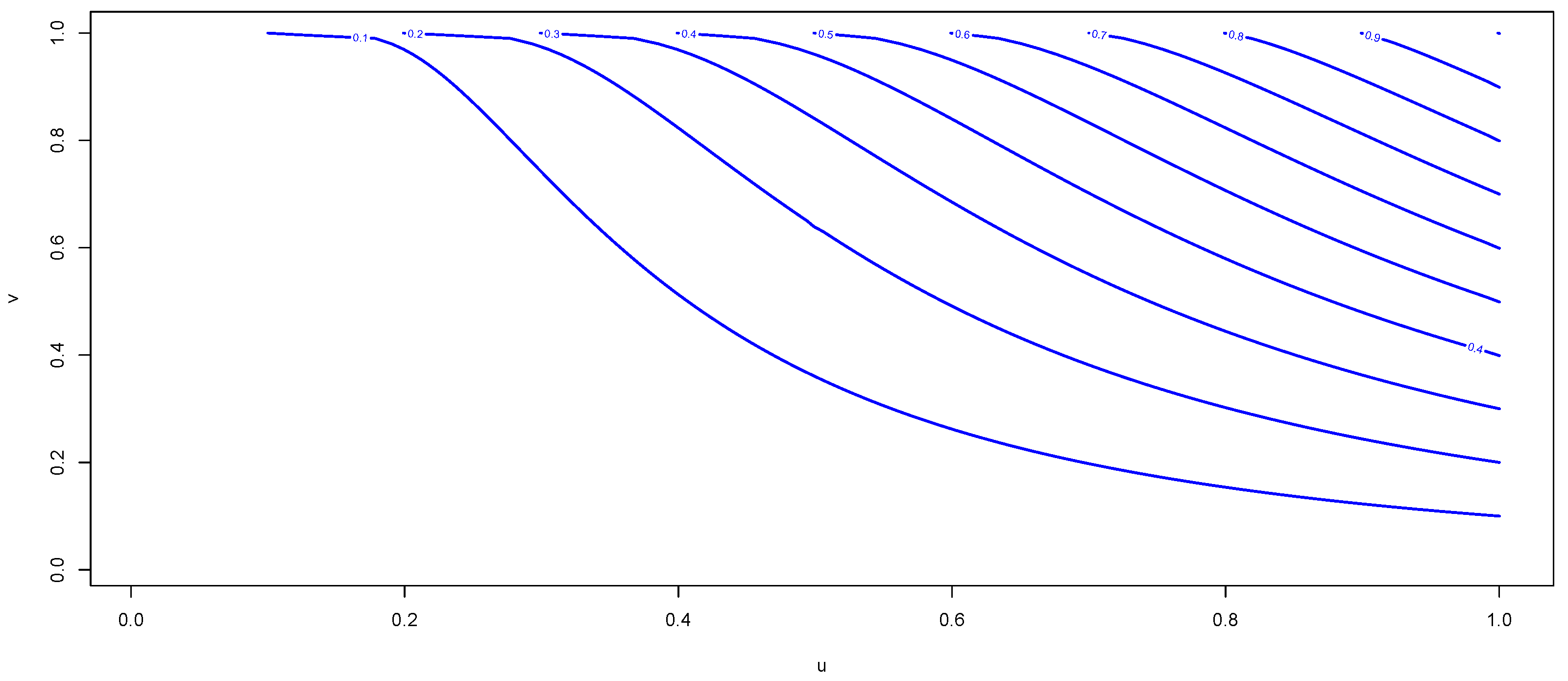
Then, by Sklar’s theorem, the implied copula function is grasped from (28). One has
The curve of the copula function in (29) is plotted in Figure 5, and also, the contour lines associated with this copula function are drawn in Figure 6.
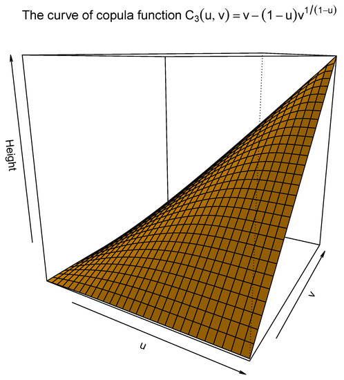
Figure 5.
The curve of the implied copula function .
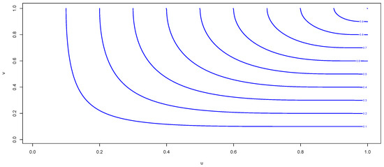
Figure 6.
Copula contour plot of .
Let us suppose that with being an increasing function and let be a decreasing function. Then, consider the case where
In this case, as with previously derived cases, . From (30), we obtain and for all . The s.f. of T by using (20) and taking X as an exponential random variable with c.d.f. where is acquired as
By an application of (10) when X follows the c.d.f. , then
By appealing to (31), the c.d.f. of in (32) is rewritten as
Then, the implied copula function is obtained from (33) by using Sklar’s theorem. One gets
The curve of the copula function in (34) is plotted in Figure 7, and furthermore, the contour lines of this copula function are drawn in Figure 8.
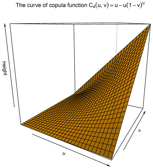
Figure 7.
The curve of the implied copula function .
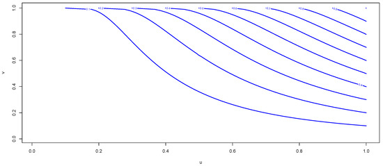
Figure 8.
Copula contour plot of .
It is worth mentioning that in the multiplicative degradation model, , which assumes that satisfies one of the four models considered, and the copula functions are not affected by the form of a monotonic mean degradation function nor by the form of the decreasing function . Nevertheless, the implicit copula function changes when either the direction of monotonicity of is reversed or when the formation of is changed. However, additive degradation models may not fall under this general rule.
In the case of the additive degradation model , we show that when is a function of , the resulting copula function is not affected by the shape of the decreasing function . In the rest of the paper, we discuss copula functions arising from additive degradation models. Let be a decreasing function. We consider
where h is an appropriate bivariate function. We assume that , where is a true function. Note that the function h and the function must satisfy some boundary conditions for and , which depend on the limiting behavior of the probability in and and further when and and also the limiting behavior of the function in and , respectively. Then, the implied survival function is obtained as
where in which X follows the c.d.f. . Notice that has to be monotonically decreasing in order for in (36) to be valid as a distribution function. The joint c.d.f. of T and X in view of (11) is acquired as
where when . Let us observe that Equation (36) concludes that for every and, therefore, for every . By substituting and in Equation (37) and then using Sklar’s theorem, the copula function is derived as
In the particular cases and , when is an increasing function and also the particular cases and in the case of the multiplicative degradation model, the copula functions in (19), (24), (29), and (34) presented. However, in view of (38), the derivation of explicit copula functions in the additive degradation model depends on .
4. Discussion
The copula functions that are generated by the time-to-failure models with a deterministic effect of degradation on failure (see Section 2) persuade the random variation and the lifetime to have more severe dependencies in comparison with the copula functions generated by dynamic time-to-failure models (see Section 3). The former copula functions are the cases when high-reliability devices for which a gradual failure are considered, whereas the latter copula functions are related to the devices where the possibility for both gradual failure and sudden failure is considered. The multiplicative degradation model provides copulas with a closed-form expression, but the additive degradation model generates copula functions that do not have a closed-form expression. Whether the functional form has for other possible degradation models an influence on the dependency between X and T and the extent to which the corresponding dependencies are affected by a variety of other degradation models can be recognized by developing (13) and (14). In this framework, as observed in the generated copula functions of T and X in the multiplicative degradation model, there is no dependence parameter to make variations in dependencies between T and X. This parameter can be produced either as a result of an external source or from the functional relation provides. On the other hand, there are a variety of candidates for the distribution of the random variation X: for example, the Weibull, gamma, and log-logistic distributions (see, for instance, Bae et al. [22]) under which implied lifetime distributions are obtained. Intuitively, it may be apparent that when any choice is made for the distribution of X, the copula function of T and X is not affected, since the copula function indeed allows us to separate the effect of marginal distributions from that of the function representing the dependence structure. Therefore, the copula function determines a novel perspective on a given degradation model, as it can be characterized uniquely by the structure of the model. In general, the literature on copula theory partly includes the methods of construction of new copulas of two dependent random variables (cf. Balakrishnan and Lai [27], Mesiar et al. [28], Durante et al. [29], Bedford and Wilson [30], Giakoumakis and Papadopoulos [31], and Alshehri and Kayid [32]). In turn, this paper also plays its role in the study of the generation of new copulas in the context of degradation models.
5. Concluding Remarks
The copula function for the random pair , where X is a random variation around representing the underlying mean degradation path, and T is either the implied random lifetime under the multiplicative degradation model or the additive degradation model , has been determined in this work. Both the cases where the degradation plays a definite role in the failure of the component and the cases where the degradation plays an uncertain competing role in the failure of the component have been considered. In the latter case, the implied lifetime distribution depends on the probability , which assumes certain constructions such as and in situations where increases in t and and when decreases in t. It was found that the derived copula functions in the case of the multiplicative degradation model do not depend on and , and thus, the dependence aspects between X and T are explicitly addressed. The copula functions in this case are also known not to be affected by other parameters. In the additive degradation model, the copula function with respect to T and X cannot be obtained exactly considering the above four constructions of and needs more restrictive conditions to be independent of both and . The conclusion is that the copula function in the additive degradation model is more dynamic compared to the copula function in the multiplicative degradation model.
In the future of this study, using the dependence measures of the derived copula functions, comparisons of copula functions can be made based on these measures. Partial dependencies between T and X can be detected. Possible extensions to multivariate cases and the derivation of multivariate copulas can be considered for the case where the degradation model consists of additional random components besides the random variation around the mean degradation path.
Author Contributions
Conceptualization, L.A. and M.K.; methodology, M.K.; software, L.A.; validation, M.K.; formal analysis, M.K.; investigation, L.A.; resources, L.A. and M.K.; writing—original draft preparation, L.A.; writing—review and editing, M.K.; visualization, M.K.; supervision, M.K.; project administration, M.K.; funding acquisition, M.K. All authors have read and agreed to the published version of the manuscript.
Funding
This work is supported by the Researchers Supporting Project number (RSP-2022/392), King Saud University, Riyadh, Saudi Arabia.
Institutional Review Board Statement
Not applicable.
Informed Consent Statement
Not applicable.
Data Availability Statement
Not applicable.
Acknowledgments
The author thanks three anonymous referees for their useful comments and suggestions that led to this improved version. The author acknowledges financial support from the Researchers Supporting Project number (RSP-2022/392), King Saud University, Riyadh, Saudi Arabia.
Conflicts of Interest
The authors declare no conflict of interest.
References
- Nelsen, R.B. An Introduction to Copulas; Springer Science and Business Media: Berlin/Heidelberg, Germany, 2007. [Google Scholar]
- Genest, C. Frank’s family of bivariate distributions. Biometrika 1987, 74, 549–555. [Google Scholar] [CrossRef]
- Joe, H. Multivariate Models and Dependence Concepts; Chapman and Hall: London, UK, 1997. [Google Scholar]
- Nadarajah, S.; Mitov, K.; Kotz, S. Local dependence functions for extreme value distributions. J. Appl. Stat. 2003, 30, 1081–1100. [Google Scholar] [CrossRef]
- Durante, F. A new family of symmetric bivariate copulas. Comptes Rendus Math. 2007, 344, 195–198. [Google Scholar] [CrossRef]
- Tang, X.S.; Li, D.Q.; Zhou, C.B.; Zhang, L.M. Bivariate distribution models using copulas for reliability analysis. Proc. Inst. Mech. Eng. Part O J. Risk Reliab. 2013, 227, 499–512. [Google Scholar] [CrossRef]
- Fréchet, M. Sur les Tableaux Dont les Marges et des Bornes Sont Données; Revue de l’Institut International de Statistique: The Hague, The Netherlands, 1960; pp. 10–32. [Google Scholar]
- Genest, C.; Nešlehová, J.; Quessy, J.F. Tests of symmetry for bivariate copulas. Ann. Inst. Stat. Math. 2012, 64, 811–834. [Google Scholar] [CrossRef]
- Ye, Z.S.; Xie, M. Stochastic modelling and analysis of degradation for highly reliable products. Appl. Stoch. Models Bus. Ind. 2015, 31, 16–32. [Google Scholar] [CrossRef]
- Valdez-Flores, C.; Feldman, R.M. A survey of preventive maintenance models for stochastically deteriorating single-unit systems. Nav. Res. Logist. 1989, 36, 419–446. [Google Scholar] [CrossRef]
- Kharoufeh, J.P.; Cox, S.M. Stochastic models for degradation-based reliability. IIE Trans. 2005, 37, 533–542. [Google Scholar] [CrossRef]
- Park, C.; Padgett, W.J. Stochastic degradation models with several accelerating variables. IEEE Trans. Reliab. 2006, 55, 379–390. [Google Scholar] [CrossRef]
- Gebraeel, N.; Pan, J. Prognostic degradation models for computing and updating residual life distributions in a time-varying environment. IEEE Trans. Reliab. 2008, 57, 539–550. [Google Scholar] [CrossRef]
- Kharoufeh, J.P.; Solo, C.J.; Ulukus, M.Y. Semi-Markov models for degradation-based reliability. IIE Trans. 2010, 42, 599–612. [Google Scholar] [CrossRef]
- Jiang, L.; Feng, Q.; Coit, D.W. Reliability and maintenance modeling for dependent competing failure processes with shifting failure thresholds. IEEE Trans. Reliab. 2012, 61, 932–948. [Google Scholar] [CrossRef]
- Peng, C.Y.; Tseng, S.T. Statistical lifetime inference with skew-Wiener linear degradation models. IEEE Trans. Reliab. 2013, 62, 338–350. [Google Scholar] [CrossRef]
- Chen, D.G.; Lio, Y.; Ng, H.K.T.; Tsai, T.R. (Eds.) Statistical Modeling for Degradation Data; Springer: Singapore, 2017. [Google Scholar]
- Chen, P.; Ye, Z.S. Uncertainty quantification for monotone stochastic degradation models. J. Qual. Technol. 2018, 50, 207–219. [Google Scholar] [CrossRef]
- Bressi, S.; Santos, J.; Losa, M. Optimization of maintenance strategies for railway track-bed considering probabilistic degradation models and different reliability levels. Reliab. Eng. Syst. Saf. 2021, 207, 107359. [Google Scholar] [CrossRef]
- He, L. Objective Bayesian analysis of accelerated degradation models based on Wiener process with correlation. Commun. Stat.-Theory Methods 2021, 2021, 1957111. [Google Scholar] [CrossRef]
- Liu, H.; Huang, J.; Guan, Y.; Sun, L. Accelerated degradation model of nonlinear wiener process based on fixed time index. Mathematics 2019, 7, 416. [Google Scholar] [CrossRef] [Green Version]
- Bae, S.J.; Kuo, W.; Kvam, P.H. Degradation models and implied lifetime distributions. Reliab. Eng. Syst. Saf. 2007, 92, 601–608. [Google Scholar] [CrossRef]
- Albabtain, A.A.; Shrahili, M.; Alshagrawi, L.; Kayid, M. A dynamic failure time degradation-based model. Symmetry 2020, 12, 1532. [Google Scholar] [CrossRef]
- Kayid, M.; Alshagrawi, L. Reliability aspects in a dynamic time-to-failure degradation-based model. Proc. Inst. Mech.Eng. Part O J. Risk Reliab. 2021, 8, 1748006X211064092. [Google Scholar] [CrossRef]
- Izadkhah, S.; Amini, M.; Borzadaran, G.M. Preservation of dependence concepts under bivariate weighted distributions. Commun. Stat.-Theory Methods 2016, 45, 4589–4599. [Google Scholar] [CrossRef]
- Li, X.; Yan, R.; Zhao, Y. Aging properties of the lifetime in simple additive degradation models. J. Syst. Sci. Complex. 2011, 24, 753–760. [Google Scholar] [CrossRef]
- Balakrishnan, N.; Lai, C.D. Construction of bivariate distributions. In Continuous Bivariate Distributions; Springer: New York, NY, USA, 2009; pp. 179–228. [Google Scholar]
- Mesiar, R.; Komornik, J.; Komornikova, M. On some construction methods for bivariate copulas. In Aggregation Functions in Theory and in Practise; Springer: Berlin/Heidelberg, Germany, 2013; pp. 39–45. [Google Scholar]
- Durante, F.; Sanchez, J.F.; Flores, M.U. Bivariate copulas generated by perturbations. Fuzzy Sets Syst. 2013, 228, 137–144. [Google Scholar] [CrossRef]
- Bedford, T.; Wilson, K.J. On the construction of minimum information bivariate copula families. Ann. Inst. Stat. Math. 2014, 66, 703–723. [Google Scholar] [CrossRef] [Green Version]
- Giakoumakis, S.; Papadopoulos, B. Novel Construction of Copulas Based on (α,β) Transformation for Fuzzy Random Variables. J. Math. 2021, 2021, 4310675. [Google Scholar] [CrossRef]
- Alshehri, M.A.; Kayid, M. Copulas generated by mixtures of weighted distributions. AIMS Math. 2022, 7, 8953–8974. [Google Scholar] [CrossRef]


Publisher’s Note: MDPI stays neutral with regard to jurisdictional claims in published maps and institutional affiliations. |
© 2022 by the authors. Licensee MDPI, Basel, Switzerland. This article is an open access article distributed under the terms and conditions of the Creative Commons Attribution (CC BY) license (https://creativecommons.org/licenses/by/4.0/).