An Application of the Kalman Filter Recursive Algorithm to Estimate the Gaussian Errors by Minimizing the Symmetric Loss Function

Abstract

Kalman filtering is a linear quadratic estimation (LQE) algorithm that uses a time series of observed data to produce estimations of unknown variables. The Kalman filter (KF) concept is widely used in applied mathematics and signal processing. In this study, we developed a methodology for estimating Gaussian errors by minimizing the symmetric loss function. Relevant applications of the kinetic models are described at the end of the manuscript.

1. Introduction

Linear quadratic estimation (LQE) is a statistical method with many technological applications. The most common applications of LQE are for navigation, guidance, and the control of vehicles [1]. Other applications [2,3] are based on the lag between the issuing signals and receiving a response, in which the Kalman filter (KF) makes assessments of the condition of the framework and issues directions.

In general, a KF assumes that the noise is normally (Gaussian) distributed and the observation models are linear [4]. Furthermore, the filter gives the posterior conditional probability estimate in the case when the errors follow a Gaussian distribution.

Over the past few decades, generalizations of and extensions to the KF method have been established, such as the unscented Kalman filter (UKF) and the extended Kalman filter (EKF), which both work on nonlinear systems [5,6]. EKF is probably the most widely used estimation algorithm for nonlinear systems [7].

The KF uses a dynamic model, known control inputs, and multiple consecutive measurements to make an estimate of its varying quantities, which leads to a better estimation than if they were obtained by using one measurement alone [8,9,10].

The Kalman filter is a productive recursive filter that evaluates the inward condition of a direct powerful framework from a progression of noisy estimations. It is utilized in a wide scope of econometric and engineering applications ranging from radar and computer vision to estimations of basic macroeconomic models [11,12], and is an important tool in control system engineering and control framework design. Together with the linear quadratic regulator (LQR), the KF determines the solutions of a direct quadratic Gaussian control issue.

Other related works in the mathematics field have been carried out as well [13,14,15]. The most representative works were [16,17,18]. Some mathematical researchers [19,20] proposed the use of a KF for the elimination of noise. An interesting approach [21] uses the extended KF for linearizing the nonlinear systems while improving the applicability of these methods.

Anderson et al. [22] presented the theory and applications of Kalman filtering in a unified and organized fashion, which encompassed major contributions by a substantial number of researchers of this topic. Jazwinski [23] took the Bayesian point of view regarding filtering, while other economists [24,25] set a procedure for the frequency domain design of statically optimal filters.

Starting from what is already known in this area, the novelty of this study consists of using a recursive algorithm of the Kalman filter, the semigroup of the Hamiltonian matrices, and the contraction property to estimate the Gaussian errors. The main difference between our work and classical approaches, such as EKF and LQE, is that it handles the time-varying measurement uncertainty. For this, the covariance matching approach is used to update the observation covariance matrix.

The rest of this paper is organized as follows. The methodology and the formulation of the system equations are described in Section 2. Section 2 also describes the KF model, the general case of the KF, and the Gaussian case. The subsequent section, Section 3, describes the semigroup of the Hamiltonian matrices and the contraction property. The results, including the need for the KF-based techniques under different conditions for the numerical and experimental study, are presented in Section 3. Based on the observed results, some conclusions and areas for future work, as well as possible applications of the proposed methodology, are identified in the last section of the paper.

2. Materials and Methods

2.1. The Kalman Filter Model

The KF is based on the following mathematical theory. Consider B_m = 1, 2, 3, … data observed from p × 1 vectors. B_m is a sequence that is presumed to have the following distribution:

B_m = D_m + φ_m = Z_mA_m + φ_m,

where

• φ_m—white noise
• D_m—carrier signal.

In this regard, the dynamic representation is as follows:

D_m = Z_mA_m, m = 1, 2, 3….

whose factors are defined below.

Next, we continue with an observed data model:

B_m = Z_mA_m + φ_m.

(1)

Equation (1) is related to the p × 1 vector of B_m data points, with an r × 1 A_m vector. In this case, Z_m is a p × r matrix, while φ_m is a p × 1 vector with E[φ_m] = 0 and Var[φ_m] = M_m.

The vector A_m is not straightforwardly observable, but we could assume that it follows a Markov chain process of order 1, i.e.,

A_m = X_mA_m−1 + θ_m, m = 1, 2, 3, …

(2)

The states’ behavior is described by Equation (2). In this case, X_m is an r × r matrix and θ_m is an r × 1 error vector, which is not correlated with θ_m since E[θ_m] = 0 and Var[θ_m] = P_m.

A₀, the initial vector, was assumed to have:

E[A₀] = x₀ and Var[A₀] = Q₀.

(3)

Furthermore, we assumed that the error terms were not two-by-two correlated, i.e.,

E[θ_nφ’_d] = 0 for all n, d = 1, 2, 3, …

(4)

and

E[θ_nA_0′] = 0 and E[φ_nA_0′] = 0 for all n = 1, 2, 3, …

(5)

We also assumed that the matrices X_m, M_m, P_m, and Z_m, as defined before, are not random matrices. The above two statements (1) and (2) reveal that A_m could be constructed as a linear combination of θ_d and φ_d, for d ≤ m − 1 and A₀ for any m.

2.2. The General Case of the Kalman Filter

From the least-squares class of estimators, the KF is a recursive estimator.

The matrices X_m, M_m, P_m, and Z_m are presumed to be known for any m.

Consider a sequence Γ_m, which includes all the data observations recorded until moment m, inclusively.

Consider now an optimal estimator x_m|m of A_m based on the data observations of Γ_m. The r × r matrix of the mean of the squared errors (EPM) of x_m|m is:

Q_m|m = E[(A_m − x_m|m)(A_m − x_m|m)’],

(6)

where “ ’ ” stands for the transpose of a matrix.

Considering x_m−1|m−1 and Q_m−1|m−1, the estimators x_m|m−1 and Q_m|m−1 of A_m and Q_m|m, which are based on the data points of Γ_m−1, can be calculated from the prediction formulas:

x_m|m−1 = X_m x_m−1|m−1 + θ_m, for m = 1, 2, 3, …

(7)

and

Q_m|m−1 = E[(A_m – x_m|m−1)(A_m – x_m|m−1)’]

= E[(X_mA_m−1 + θ_m – X_mx_m−1|m−1)(X_mA_m−1 + θ_m – X_mx_m−1|m−1)’]

= E[(X_m(A_m−1 – x_m−1|m−1) + θ_m)(X_m(A_m−1 − x_n−1|n−1) + θ_m)’]

= X_mE[(A_m−1 – x_m−1|m−1)(A_m−1 – x_m−1|m−1)’]X’_m + E[θ_mθ’_m],

i.e.,

Q_m|m−1 = X_mQ_m−1|m−1X’_m + P_m, for m = 1, 2, 3, …

(8)

By (4) and (5), the average of the connected terms of the multiplication is zero.

Since A_m−1 is a linear combination of the terms θ_d and φ_d, d ≤ m − 1, and the A₀ term is also not correlated with φ_m.

The equations (7) and (8) above represent the KF. Given A₀ and Q₀, the KF gives the optimal estimator of the state when new data points are accessible.

2.3. The Gaussian Case

Now, we consider the following system:

A_m = X_mA_m−1 + θ_m,

B_m = Z_mA_m + φ_m, m ≥ 1,

(9)

where

• X_m and Z_m are deterministic r × r and p × r matrices, respectively, and
• A_m$\in$R^r, θ_m$\in$R^q, φ_m, and B_m$\in$R^p are random variables.

Now, we assume that the pair of vectors (θ_m,φ_m), m ≥ 1, are independent and have a Gaussian distribution with an average of 0 and a covariance matrix equal to J, where J is the unit matrix and A₀ has a Gaussian distribution with an average of a₀ and a covariance matrix Q₀. We then assume that the determinant of X_m is not zero, m ≥ 1.

For any m ≥ 1, let an N_m σ-algebra be generated by B₁, …, B_m [26] and

$${\hat{\mathrm{A}}}_{\mathrm{m}}=\mathrm{E}[{\mathrm{A}}_{\mathrm{m}}|{\mathrm{N}}_{\mathrm{m}}],$$

(10)

$${\mathrm{Q}}_{\mathrm{m}}=\mathrm{E}\left(\right({\mathrm{A}}_{\mathrm{m}}-{\hat{\mathrm{A}}}_{\mathrm{m}}\left)\right({\mathrm{A}}_{\mathrm{m}}-{\hat{\mathrm{A}}}_{\mathrm{m}})\prime |{\mathrm{N}}_{\mathrm{m}}).$$

(11)

If N_m is known, ${\hat{\mathrm{A}}}_{\mathrm{m}}$ is the best estimator of A_m and Q_m is the conditional variance–covariance matrix of the errors.

Now, we consider Q, respectively Q₀, which is the set of symmetric matrices that are non-negatively defined (respectively positively defined) and of r × r dimensions. For any Q$\in Q$ and m ≥ 1, we then define:

ξ_m(Q) = (X_mQX’_m + J)(J + S_m + S_mX_mQX’_m)⁻¹,

(12)

where S_m = Z’_mZ_m and J is the unit matrix of order r. It follows that ξ_m takes P₀ into itself.

The basic result shown above is related to the fact that the applications ξ_m, m ≥ 1, are contractions in Q₀ if we enhance Q₀ with the Riemann measurement δ [27], which is invariant to conjugacy. Furthermore, the contractions could be strict or uniform, depending on the controllability and observability properties of the above system (9).

To demonstrate the results in this view, we considered the symplectic group of matrices. The matrices are invariant to P₀. In this view, they could be considered a generalization of the Perron–Frobenius theorem. In some sense, the study of Bougerol [28] is elementary.

The symplectic matrices utilize some of the already existing ideas [29]. The semigroup Σ was induced by Wojtkowsky [30] in a similar context. Finally, we note that the Riccati transformation [31] has a contractibility property, which is a generalization of the positive matrices under a Hilbert space metric [32].

3. Applications to Kinetic Models

3.1. A Recursive KF Algorithm Application

We considered an object moving along a straight line. Its movements are captured by a video camera. The object is moving along a straight line, with random acceleration a_t, and ${\mathsf{\Delta }}_t$is the time interval. Its location is described by the x-coordinate. We also assumed that the acceleration has a Gaussian distribution with zero mean and constant variance (${\sigma }_a^2$). The position of the object, denoted as y_t, is also noisy (Gaussian with zero mean and constant variance). We denote the variance as ${\sigma }_y^2$.

The state vector of this motion is given by $v_t$ = ($x_t$,$v_t$), where the speed is the first derivative of the distance, i.e., $v_t={\dot{x}}_t$.

We also assumed that there was no process control and get:

$$x_t=\left(\begin{array}{cc}1& {\Delta }_t\\ 0& 1\end{array}\right)\left(\begin{array}{c}{x}_{t-1}\\ v_{t-1}\end{array}\right)+a_t\left(\begin{array}{c}\frac{{\Delta }_t{}^2}{2}\\ {\Delta }_t\end{array}\right)=F_t{x}_{t-1}+w_t,Q_t=\mathrm{var}(w_t),$$

(13)

where

• $F_t$ is a known state transition matrix applied to the t − 1 state x_t−1,
• $Q_t$ is the variance matrix, and
• $w_t$ is a process noise vector, which has the joint distribution as a multivariate Gaussian with a variance matrix $Q_t$ and ${\mu }_{i,t}=E\left[w_{i,t}\right]=0$ for $i=\overline{1,n}$.

Now, let $G_t={\left(\frac{{\Delta }_t{}^2}{2},{\Delta }_t\right)}^T$. Then, we get:

$$Q_t=E\left[w_t,w_t^T\right]=G_{t}E\left[a_t^2\right];G_t^T={\sigma }_a^2{G}_t{G}_t^T={\sigma }_a^2\left[\begin{array}{cc}\frac{{\Delta }_t{}^4}{4}& \frac{\Delta t^3}{2}\\ \frac{{\Delta }_t{}^3}{2}& {\Delta }_t{}^2\end{array}\right].$$

(14)

This means that F_t, Q_t, and G_t are independent of t. Hence, we will call them just F, Q, and G.

To measure the object’s position at time t, we get:

$$y_t=\left(\begin{array}{c}{v}_t\\ 0\end{array}\right)\left(\begin{array}{cc}1& 0\\ 0& 0\end{array}\right)x_t=v_t+H_t\cdot x_t,$$

(15)

where

• v_t is the observation noise and
• H_t is an observation matrix.

Hence, the variance matrix is:

$$R=E\left[v_t{v}_t^T\right]=\left(\begin{array}{cc}{\sigma }_y^2& 0\\ 0& 0\end{array}\right).$$

(16)

We denote ${\hat{x}}_{t|t}$ as the estimate of state x_t at time t and $P_{t|t}$ as the variance matrix of the error $x_t-{\hat{x}}_{t|t}$. Our goal was to minimize $P_{t|t}$.

The initial position of the object is ${\hat{x}}_{0|0}={(0,0)}^T$. If this position vector is known accurately, then the variance matrix is zero, i.e.,

$$P_{0|0}=\left(\begin{array}{cc}0& 0\\ 0& 0\end{array}\right);$$

otherwise, we will have that:

$$P_{0|0}=\left(\begin{array}{cc}a& 0\\ 0& a\end{array}\right),$$

where a is real and suitably large, a > 0.

When t = 1, we first predicted ${\hat{x}}_{1|0}$ and computed its variance matrix $P_{1|0}$ by using the prediction equations:

$${\hat{x}}_{t|t-1}=F_t{\hat{x}}_{t-1|t-1}+B_t{u}_t=F{\hat{x}}_{t-1|t-1},$$

(17)

$$P_{t|t-1}=F_t{P}_{t-1|t-1}{F}_t^T+Q_t=F{P}_{t-1|t-1}{F}_t^T+Q_t=F{P}_{t-1|t-1}+Q,$$

(18)

where $B_t$ is the control matrix, which is applied to a control vector u_t.

We then calculated the auxiliary data S₁ and z₁ from the equations:

$${\tilde{z}}_t=y_t-H_t{\hat{x}}_{t|t-1}=y_t-H{\hat{x}}_{t|t-1},$$

(19)

$$S_t=H_t{P}_{t|t-1}{H}_t^T+R_t=H{P}_{t|t-1}{H}^T+R,$$

(20)

where R_t is the variance matrix of a multivariate Gaussian distribution vector v_t.

Then, we could compute the optimal Kalman gain K₁ and the position vector ${\hat{x}}_{1|1}$ using the equations:

$${\hat{x}}_{t|t}={\hat{x}}_{t|t-1}+K_t{\tilde{z}}_t,$$

(21)

$$K_t=P_{t|t}{H}_t^T{S}_t^{-1}=P_{t|t-1}{H}^T{S}_t^{-1}.$$

(22)

Finally, we could compute P_1|1 to prepare for time t = 2 by using the following equation:

$$P_{t|t}=\left(I-K_t{H}_t\right)P_{t|t-1}=\left(I-K_{t}H\right)P_{t|t-1},$$

(23)

which minimizes the variance matrix $P_{t|t}$.

3.2. EKF Recursive Algorithm Application

We extended our previous example of an object moving along a straight line by adding the orientation of the vehicle θ to the position vector (x,y). Then, we estimated the state vector p, i.e., p = (x,y,θ).

The kinematic model is given by the following system:

$$\{\begin{array}{l}{x}_t=x_{t-1}+v_t\cdot {\Delta }_t\cdot \cos \left({\theta }_{t-1}+w_t\cdot \frac{{\Delta }_t}{2}\right),\\ y_t=y_{t-1}+v_t\cdot {\Delta }_t\cdot \sin \left({\theta }_{t-1}+w_t\cdot \frac{{\Delta }_t}{2}\right),\\ {\theta }_t={\theta }_{t-1}+w_t\cdot {\Delta }_t,\end{array}$$

(24)

where Δ_t is the time interval, while v and w are the speed and the yaw rate of the vehicle. We also denote $\hat{v}$ and $\hat{w}$ as the speed and yaw rate measurements. We assumed that their errors followed the Gaussian distribution as $\mathsf{\Delta }{v}_t~N\left(0,{\sigma }_{v_t}^2\right)$ and $\mathsf{\Delta }{w}_t~N\left(0,{\sigma }_{w_t}^2\right)$.

Now, suppose that the vehicle is equipped with a GPS, and the GPS measurements are denoted by vector z with a measurement model given by:

$${\mathit{z}}_t=\mathit{H}{\mathit{p}}_t+{\gamma }_t,\mathit{H}=\left(\begin{array}{ccc}1& 0& 0\\ 0& 1& 0\end{array}\right),$$

(25)

where $\gamma ~N\left(0,{\sigma }_{\gamma }^2\right)$ is the measurement error that follows a Gaussian distribution with zero mean and variance ${\sigma }_{\gamma }^2$.

This is an EKF model, which could be locally linearized as follows:

$$\left(\begin{array}{c}{x}_t\\ y_t\\ {\theta }_t\end{array}\right)\approx \left(\begin{array}{c}{\overline{x}}_t\\ {\overline{y}}_t\\ {\overline{\theta }}_t\end{array}\right)+\mathit{A}\left({\mathit{p}}_{t-1},{\mathit{u}}_t\right)\left(\begin{array}{c}\mathsf{\Delta }{x}_{t-1}\\ \mathsf{\Delta }{y}_{t-1}\\ \mathsf{\Delta }{\theta }_{t-1}\end{array}\right)+\mathit{B}\left({\mathit{p}}_{t-1},{\mathit{u}}_t\right)\left(\begin{array}{c}\mathsf{\Delta }{v}_t\\ \mathsf{\Delta }{\omega }_t\end{array}\right),$$

$$\{\begin{array}{l}{\overline{x}}_t=x_{t-1}+v_t\cdot {\Delta }_t\cdot \cos \left({\theta }_{t-1}+w_t\cdot \frac{\mathsf{\Delta }t}{2}\right),\\ {\overline{y}}_t=y_{t-1}+v_t\cdot {\Delta }_t\cdot \sin \left({\theta }_{t-1}+w_t\cdot \frac{\mathsf{\Delta }t}{2}\right),\\ {\overline{\theta }}_t={\theta }_{t-1}+w_t\cdot {\Delta }_t,\end{array}$$

$$\mathit{A}\left({\mathit{p}}_{t-1},{\mathit{u}}_t\right)=\left(\begin{array}{ccc}1& 0& -v_t\cdot {\Delta }_t\cdot \sin \left({\theta }_{t-1}+w_t\cdot \frac{\mathsf{\Delta }t}{2}\right)\\ 0& 1& v_t\cdot {\Delta }_t\cdot \cos \left({\theta }_{t-1}+w_t\cdot \frac{\mathsf{\Delta }t}{2}\right)\\ 0& 0& 1\end{array}\right),$$

$$\mathit{B}\left({\mathit{p}}_{t-1},{\mathit{u}}_t\right)=\left(\begin{array}{cc}\Delta t\cdot \cos \left({\theta }_{t-1}+w_t\cdot \frac{{\Delta }_t}{2}\right)& -v_t\cdot \mathsf{\Delta }{t}^2\cdot \sin \left({\theta }_{t-1}+w_t\cdot \frac{{\Delta }_t}{2}\right)\\ \Delta t\cdot \sin \left({\theta }_{t-1}+w_t\cdot \frac{{\Delta }_t}{2}\right)& v_t\cdot \mathsf{\Delta }{t}^2\cdot \cos \left({\theta }_{t-1}+w_t\cdot \frac{{\Delta }_t}{2}\right)\\ 0& \mathsf{\Delta }t\end{array}\right),$$

(26)

where ${\mathit{u}}_t=\left(v_t,w_t\right)$.

As we can see, the matrices $\mathit{A}\left({\mathit{p}}_{t-1},{\mathit{u}}_t\right)$ and $\mathit{B}\left({\mathit{p}}_{t-1},{\mathit{u}}_t\right)$ of the state evolution function are Jacobian with respect to ${\mathit{p}}_{t-1}$ and ${\mathit{u}}_t$, respectively.

Hence, we have a locally linearized EKF model. The prediction of the state vector is:

$$\left(\begin{array}{c}{\overline{x}}_t\\ {\overline{y}}_t\\ {\overline{\theta }}_t\end{array}\right)=\left(\begin{array}{c}{\hat{x}}_{t-1}+{\hat{v}}_t\cdot {\Delta }_t\cdot \cos \left({\hat{\theta }}_{t-1}+{\hat{w}}_t\cdot \frac{{\Delta }_t}{2}\right)\\ {\hat{y}}_{t-1}+{\hat{v}}_t\cdot {\Delta }_t\cdot \sin \left({\hat{\theta }}_{t-1}+{\hat{w}}_t\cdot \frac{{\Delta }_t}{2}\right)\\ {\hat{\theta }}_{t-1}+{\hat{w}}_t\cdot {\Delta }_t\end{array}\right).$$

(27)

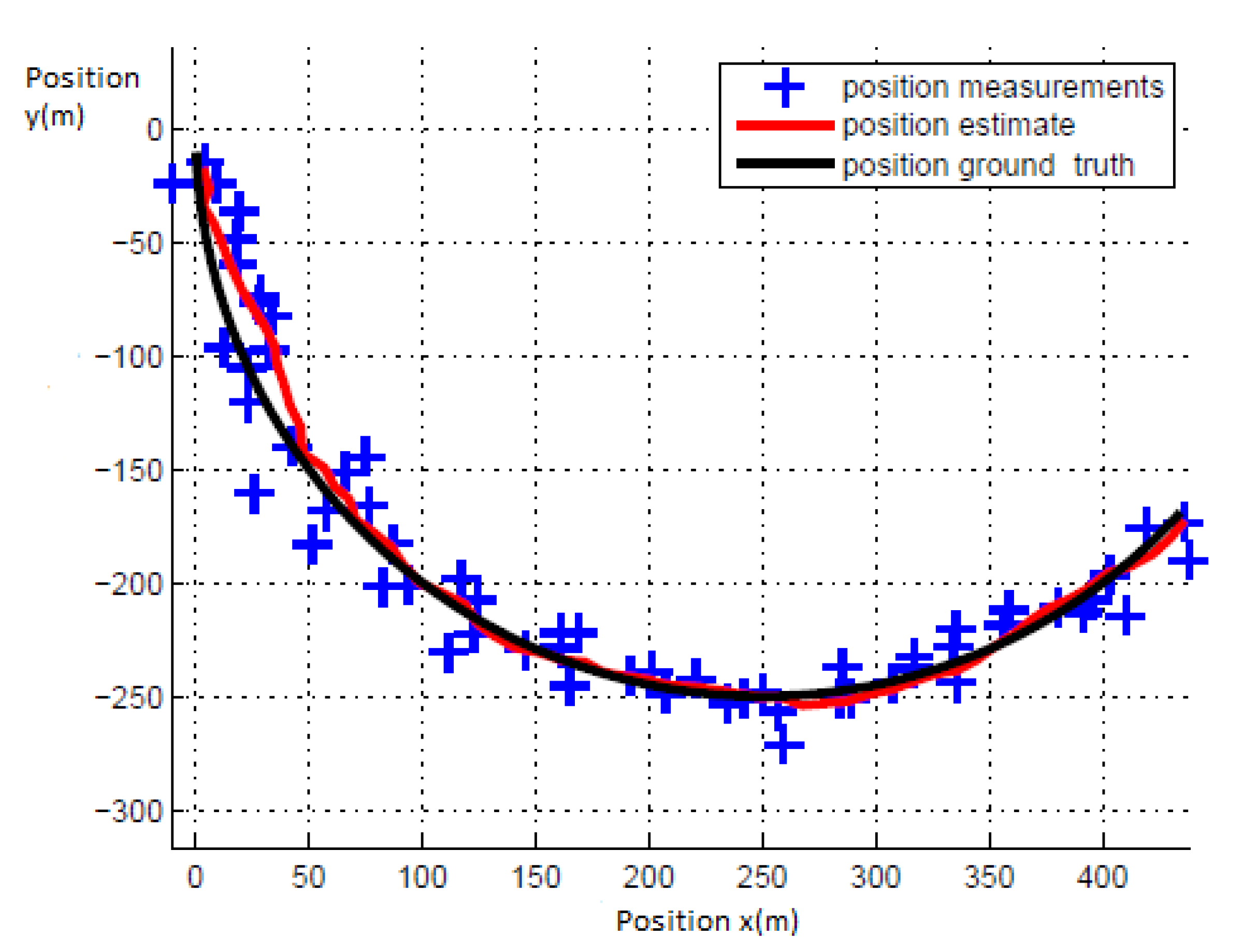
3.3. Simulation Using Synthetic Data

We tested the KF performance using synthetic data generated using model (24) and the measurement model (25). Now let:

$$\mathsf{\Delta }t=1 ,{\sigma }_w^2={0.02}^2 {\mathrm{rad}}^2/{\mathrm{s}}^2,{\sigma }_v^2={0.5}^2 {\mathrm{m}}^2/{\mathrm{s}}^2,{\sigma }_{\gamma }^2=diag\left({10}^2,{10}^2\right) {\mathrm{m}}^2.$$

Now, we set the ground truth:

$$p_0=0 ,0\mathrm{m},-\frac{\mathsf{\pi }}{2}\mathrm{rad},w_t=0.04\mathrm{rad}·\mathrm{s},v_t=10 \mathrm{m}/\mathrm{s}.$$

The yaw rate measurements and the speed measurements were synthesized according to ${\hat{w}}_t~N\left(w_t,{\sigma }_w^2\right)$ and ${\hat{v}}_t~N\left(v_t,{\sigma }_v^2\right)$.

The GPS measurements were synthesized according to ${\hat{z}}_t~N\left(p_t,{\sigma }_{\gamma }^2\right)$.

Then, the KF was applied to the synthetic data and estimates of the state of the vehicle were obtained. The results can be seen in Figure 1, in which:

• The red line represents the estimated vehicle trajectory.
• The black line stands for the ground truth of the vehicle trajectory.
• The blue crosses are the GPS measurements of the position of the vehicle.

As we can see from the above figure, the estimated trajectory of the vehicle was smoother than the jumping measurements. Figure 2 shows the results of 100 Monte Carlo trials. As we can observe, the measurement errors were larger than the estimated errors, just like in the previous example.

We also calculated the orientation estimate errors and the results of the same 100 Monte Carlo simulations are shown in Figure 3. As we can observe, these errors varied around 0.05 radians.

Hence, we concluded that, without using estimations in this application, we could not have any estimate of the vehicle’s orientation except a random guess, which could be as large as π/2 radians.

This last example shows another important utility of the estimation, i.e., a proper estimation of the Gaussian errors could reveal the state part, which is not directly measurable.

4. Discussion and Conclusions

The Kalman filter is an adequate recursive filter that evaluates the internal capacity of a linear dynamic system (LDS) using a series of error estimates. Possible applications of the KF are in economics, biology, and the environmental sciences, and it is an important topic in control systems engineering and control theory. Together with the LQR, the KF solves the linear quadratic Gaussian (LQG) control problem. The linear quadratic Gaussian controller, linear quadratic regulator, and Kalman filter are solutions to some of the most important problems in control theory.

In many applications, the few “detectable” measured parameters are smaller than the internal state. In this situation, the Kalman filter could estimate the entire internal state by combining a series of measurements.

The Kalman filter could be adapted to a wide variety of economic applications. It is mainly an ordinal least-square (OLS) procedure that gives the minimum mean square estimators (MMSE) under the Gaussian assumption. Even when the normality assumption is waived, the Kalman filter minimizes any symmetric loss function. The KF is not only used directly in economic problems but it could also be used as a background to other estimation techniques, such as the estimation of Markov switching models or the quasi-maximum likelihood estimation procedure.

In the environmental sciences, the Kalman filter has wide applications in the areas of the pollution of aquatic systems, measuring atmospheric pollution, environmental policy management, and forecasting hurricanes [33,34]. The KF could also be used to estimate the temporal variations in associations between the radial growth of black oak and physiologically based climate indices [35,36]. In biology, biological samples and bacteriological infections could be detected using a multi-process Kalman filter to provide an online estimate of the inflection point of changes in the growth of an organism [37].

A wide collection of Kalman filters have been developed in the past few decades from the original formulation of the Kalman filter. The information filter, Schmidt’s extended filter, or the Kalman–Bucy filter are a wide variety of filters that were developed by Thornton, Bierman, and many others. Probably the most used type of Kalman filter is the phase-locked loop (PLL), which is now omnipresent in television sets, radios, satellite communications receivers, and almost any other communications equipment. In this paper, we presented the KF model, the general case of the KF, and the Gaussian case. The semigroup of the Hamiltonian matrices and contraction property were used in the KF algorithm to estimate the Gaussian errors.

The main result of this study was the use of a recursive algorithm of the Kalman filter to estimate the Gaussian errors.

Several possible variations of our approach exist. Model herring inflow as a state variable and model herring inflow as pure noise with a non-zero mean or model noise as pure white (non-geometric) noise assume perfect observations of the control variables (catch and inflow). These variations were all tested and led to only small changes in the recursive algorithm fit and small variations in the parameter estimates.

The main limitation of this study came from the fact that there were not many applications of the algorithms described in the previous sections. Future work, as well as possible applications of the methodology, could be applied in mathematics, physics, and engineering research areas. Moreover, a future research topic is how to treat more general noise terms, for example, terms including unknown parameters.

References

1. Musoff, H.; Zarchan, P. Fundamentals of Kalman Filtering: A Practical Approach; American Institute of Aeronautics and Astronautics: Reston, VA, USA, 2009. [Google Scholar]
2. Wolpert, D.; Ghahramani, Z. Computational Principles of Movement Neuroscience. Nat. Neurosci. 2000, 3, 1212–1217. [Google Scholar] [CrossRef] [PubMed]
3. Hameed, Z.; Hong, Y.S.; Cho, Y.M.; Ahn, S.H.; Song, C.K. Condition monitoring and fault detection of wind turbines and related algorithms: A review. Renew. Sustain. Energy Rev. 2009, 13, 1–39. [Google Scholar] [CrossRef]
4. Kalman, R.E. A New Approach to Linear Filtering and Prediction Problems. J. Basic Eng. 1960, 82, 35. [Google Scholar] [CrossRef] [Green Version]
5. Tseng, C.H.; Lin, S.F.; Jwo, D.J. Fuzzy adaptive cubature Kalman filter for integrated navigation systems. Sensors 2016, 16, 1167. [Google Scholar] [CrossRef] [Green Version]
6. Yamauchi, T. Modeling Mindsets with Kalman Filter. Mathematics 2018, 6, 205. [Google Scholar] [CrossRef] [Green Version]
7. Julier, S.J.; Uhlmann, J.K. Unscented filtering and nonlinear estimation. Proc. IEEE 2004, 92, 401–422. [Google Scholar] [CrossRef] [Green Version]
8. Singh Sidhu, H.; Siddhamshetty, P.; Kwon, J. Approximate Dynamic Programming Based Control of Proppant Concentration in Hydraulic Fracturing. Mathematics 2018, 6, 132. [Google Scholar] [CrossRef] [Green Version]
9. Song, H.; Yu, K.; Li, X.; Han, J. Error estimation of load identification based on linear sensitivity analysis and interval technique. Struct. Multidiscip. Optim. 2017, 55, 423–436. [Google Scholar] [CrossRef]
10. Ma, C.; Tuan, P.; Lin, D.; Liu, C. A study of an inverse method for the estimation of impulsive loads. Int. J. Syst. Sci. 1998, 29, 663–672. [Google Scholar] [CrossRef]
11. Ma, C.; Ho, C. An inverse method for the estimation of input forces acting on non-linear structural systems. J. Sound Vib. 2004, 275, 953–971. [Google Scholar] [CrossRef]
12. Lin, D. Input estimation for nonlinear systems. Inverse Probl. Sci. Eng. 2010, 18, 673–689. [Google Scholar] [CrossRef]
13. Kim, J.; Kim, K.; Sohn, H. Autonomous dynamic displacement estimation from data fusion of acceleration and intermittent displacement measurements. Mech. Syst. Signal. Process. 2014, 42, 194–205. [Google Scholar] [CrossRef]
14. Casciati, F.; Casciati, S.; Faravelli, L.; Vece, M. Validation of a data-fusion based solution in view of the real-time monitoring of cable-stayed bridges. Procedia Eng. 2014, 199, 2288–2293. [Google Scholar] [CrossRef]
15. Zhang, C.; Xu, Y. Structural damage identification via multi-type sensors and response reconstruction. Struct. Health Monit. 2016, 15, 715–729. [Google Scholar] [CrossRef]
16. Zhu, W.; Wang, W.; Yuan, G. An improved interacting multiple model filtering algorithm based on the cubature Kalman filter for maneuvering target tracking. Sensors 2016, 16, 805. [Google Scholar] [CrossRef] [PubMed] [Green Version]
17. Amin, M.; Rahman, M.; Hossain, M.; Islam, M.; Ahmed, K.; Miah, B. Unscented Kalman Filter Based on Spectrum Sensing in a Cognitive Radio Network Using an Adaptive Fuzzy System. Big Data Cogn. Comput. 2018, 2, 39. [Google Scholar] [CrossRef] [Green Version]
18. Giffin, A.; Urniezius, R. The Kalman Filter Revisited Using Maximum Relative Entropy. Entropy 2014, 16, 1047–1069. [Google Scholar] [CrossRef]
19. Cao, M.; Qiu, Y.; Feng, Y.; Wang, H.; Li, D. Study of Wind Turbine Fault Diagnosis Based on Unscented Kalman Filter and SCADA Data. Energies 2016, 9, 847. [Google Scholar] [CrossRef]
20. Kim, D.-W.; Park, C.-S. Application of Kalman Filter for Estimating a Process Disturbance in a Building Space. Sustainability 2017, 9, 1868. [Google Scholar] [CrossRef] [Green Version]
21. Feng, K.; Li, J.; Zhang, X.; Zhang, X.; Shen, C.; Cao, H.; Yang, Y.; Liu, J. An Improved Strong Tracking Cubature Kalman Filter for GPS/INS Integrated Navigation Systems. Sensors 2018, 18, 1919. [Google Scholar] [CrossRef] [Green Version]
22. Anderson, B.D.; Moore, J.B. Optimal Filtering; Courier Corporation: Chelmsford, MA, USA, 2012. [Google Scholar]
23. Jazwinski, A.H. Stochastic Processes and Filtering Theory; Courier Corporation: Chelmsford, MA, USA, 2007. [Google Scholar]
24. Gelb, A. Applied Optimal Estimation; MIT press: Cambridge, MA, USA, 1974. [Google Scholar]
25. Tanizaki, H. Nonlinear Filters: Estimation and Applications; Springer Science & Business Media: Berlin/Heidelberg, Germany, 2013. [Google Scholar]
26. Mihail, B.; Sorin, C. An Application of the Kalman Filter for Market Studies. Ovidius Univ. Ann. Ser. Econ. Sci. 2013, 13, 726–731. [Google Scholar]
27. Shelkovich, V.M. The Riemann problem admitting δ-, δ′-shocks, and vacuum states (the vanishing viscosity approach). J. Differ. Equ. 2006, 231, 459–500. [Google Scholar] [CrossRef] [Green Version]
28. Bougerol, P. Kalman filtering with random coefficients and contractions. Siam J. Control. Optim. 1993, 31, 942–959. [Google Scholar] [CrossRef]
29. Shayman, M.A. Phase portrait of the matrix Riccati equation. Siam J. Control Optim. 1986, 24, 1–65. [Google Scholar] [CrossRef]
30. Wojtkowski, M. Invariant families of cones and Lyapunov exponents. Ergod. Theory Dyn. Syst. 1985, 5, 145–161. [Google Scholar] [CrossRef] [Green Version]
31. Smith, D.R. Decoupling Order Reduction via the Riccati Transformation. Siam Rev. 1987, 29, 91–113. [Google Scholar] [CrossRef]
32. Birkhoff, G. Extensions of Jentzsch’s theorem. Trans. Am. Math. Soc. 1957, 85, 219–227. [Google Scholar]
33. Piegorsch, W.W.; Smith, E.P.; Edwards, D.; Smith, R.L. Statistical advances in environmental science. Stat. Sci. 1998, 13, 186–208. [Google Scholar] [CrossRef]
34. Bril, G. Forecasting hurricane tracks using the Kalman filter. Environmetrics 1995, 6, 7–16. [Google Scholar] [CrossRef]
35. LeBlanc, D.C. Spatial and temporal variations in the prevalence of growth decline in red spruce populations of the northeastern United States: Reply. Can. J. Res. 1993, 23, 1494–1496. [Google Scholar] [CrossRef]
36. Cook, E.R.; Johnson, A.H. Climate change and forest decline: A review of the red spruce case. Water Air Soil Pollut. 1989, 48, 127–140. [Google Scholar] [CrossRef]
37. Whittaker, J.; Fruhwirth-Schnatter, S. A dynamic change point model for detecting the onset of growth in bacteriological infections. Appl. Stat. 1994, 43, 625–640. [Google Scholar] [CrossRef]
Figure 1. Estimates and position measurements for one trial.
Symmetry 13 00240 g001
Figure 2. Measurement errors and position estimates of 100 Monte Carlo trials.
Symmetry 13 00240 g002
Figure 3. Orientation estimate errors for 100 Monte Carlo trials.
Symmetry 13 00240 g003
Publisher’s Note: MDPI stays neutral with regard to jurisdictional claims in published maps and institutional affiliations.