Article

An Inertial Algorithm for Solving Hammerstein Equations

Department of Pure and Applied Mathematics, Mathematics Institute, Emerging Regional Centre of Excellence (ERCE) of the European Mathematical Society (EMS), African University of Science and Technology, PMB 681, Abuja 900107, Nigeria
*
Author to whom correspondence should be addressed.
Symmetry 2021, 13(3), 376; https://doi.org/10.3390/sym13030376
Submission received: 26 January 2021 / Revised: 10 February 2021 / Accepted: 15 February 2021 / Published: 26 February 2021

Abstract

:
An inertial algorithm for solving Hammerstein equations is presented. This algorithm is obtained as a consequence of a new inertial algorithm proposed and studied for solving nonlinear equations involving operators that are m-accretive. Some strong convergence theorems are proved in real Banach spaces that are uniformly smooth. Furthermore, comparisons of the numerical performance of our algorithms with the numerical performance of some recent important algorithms are presented.
MSC:
47J05; 47H09; 47J25; 47H10; 47J20

1. Introduction

An algorithm of inertial-type is an iterative procedure in which subsequent terms are obtained using the preceding two terms. Inertial-type algorithm was proposed by Polyak [1]. Consider the dynamical system:
u ( t ) + γ u ( t ) + f ( u ( t ) ) = 0 ,
where γ > 0 and f : R n R is differentiable. The system (1) is discretized such that, having the terms z n 1 and z n , the next term z n + 1 , can be determined using
z n + 1 2 z n + z n 1 h 2 + γ z n z n 1 h + f ( z n ) = 0 , n 1 ,
where h is the step size. Equation (2) yields the following iterative algorithm:
z n + 1 = z n + β ( z n z n 1 ) α f ( z n ) , n 1 ,
where β = 1 γ h , α = h 2 and β ( z n z n 1 ) is called the inertial extrapolation term, which is intended to speed up the convergence of the sequence generated by Equation (3). Our interest in this paper is to propose inertial algorithms for solving nonlinear equations involving accretive operators. Accretive operators were introduced during the late 1960s by Browder [2] and Kato [3]. A motivation for the study of accretive maps is the fact that they appear in evolution equations in Banach spaces. Accretive operators appear also in partial differential equations. For example, consider the equation:
f t ( t , u ) f ( t , u ) = g ( f ( t , u ) ) , t 0 , u Ω , f ( t , u ) = 0 , t 0 , u Ω , f ( 0 , u ) = f 0 ( u ) , f 0 L 2 ( Ω ) ,
where Ω R n is smooth and open. Setting v ( t ) = f ( t , . ) , where
v : [ 0 , ) L 2 ( Ω )
is given by v ( t ) ( u ) = f ( t , u ) and setting h ( φ ) ( u ) = g ( φ ( u ) ) , where
h : L 2 ( Ω ) L 2 ( Ω ) ,
we see that Equation (4) reduces to the evolution equation:
v ( t ) + A v ( t ) = h ( v ( t ) ) , t 0 , v ( 0 ) = f 0 ,
where A : = is accretive.
In real Hilbert spaces, the concepts of accretivity and monotonicity coincide. However, as has been noted by Hezewinkel, Series Editor of Mathematics and Its Applications, Kluwer Academic Publishers,
“It is probably impossible to overestimate the importance of the inner product for the study of problems and phenomena which take place in a Hilbert space. However, many, and probably most, mathematical objects and models do not live in Hilbert spaces.”
(Cioranescu [4], viii)
Since monotone operators have been studied extensively in Hilbert spaces, we shall concentrate our study of accretive operators on real Banach spaces. Let A : E 2 E be a set-valued accretive operator on a real Banach space E. The Cauchy Problem for the following evolution inclusion:
0 d u d t + A u , u ( 0 ) = x , x D ( A )
has been of interest to many authors (see, e.g., [5,6]).
A map u : R + E is a solution of (5) if on any bounded subinterval of R + , it is absolutely continuous and in addition, it is differentiable a.e. on R + with u ( 0 ) = x , and satisfies the inclusion (5) a.e. on R + .
With this understanding of a solution of (5), it is known that (5) has at most one solution (see e.g., Cioranescu [4], Proposition 4.2, p. 210). At equilibrium state d u d t 0 , thus, we deduce the following from (5):
0 A u ,
whose solutions correspond to the equilibrium points of the dynamical system given in (5). Consequently, a problem of interest in the study of accretive operators is:
f i n d u D ( A ) E w i t h 0 A u .
The inclusion (7) has been considered in real Hilbert spaces and more general real Banach spaces by many authors. The well-known proximal point algorithm (PPA) of Martinet [7] has been employed for finding solutions of problem (7) involving maximal monotone operators in Hilbert spaces and the algorithm is given by:
( P P A ) x 1 H x n + 1 = J λ n A x n + e n , n 1 ,
where J λ n A = I + 1 λ n A 1 , I is the identity mapping on H, λ n > 0 is a regularizing parameter and e n is an error vector. The algorithm (8) has been studied extensively by Rockafellar [8] who proved weak convergence of the sequence generated by (8) to a solution of (7). Since then, several modifications and alternatives of the PPA have been proposed by many authors to guarantee strong convergence to a solution of the inclusion problem (7) (see, e.g., [9,10] for the progress over the years).
Motivated by the use of the resolvent operator in algorithms for solving equations involving monotone operators, some authors have introduced the resolvent operator in iterative algorithms for solving equations involving m-accretive operators. The following theorems are two of the most general results now known for approximating solutions of (7) in more general real Banach spaces.
Theorem 1
(Xu, [11]). Let E be a reflexive Banach space that has a weakly continuous duality map J with gauge φ and let A be an m-accretive operator on X such that C = D ( A ) is convex. Assume (i) lim α n = 0 and α n = (ii) lim λ n = . Given u , x 1 C , let { x n } be the sequence generated by
x n + 1 = α n u + ( 1 α n ) J λ n A x n , n 1 .
Then, the sequence { x n } converges strongly to a zero of A.
Theorem 2
(Qin and Su, [12]). Let E be a uniformly smooth real Banach space and A be an m-accretive operator in E such that A 1 ( 0 ) . Given a point u C and given { α n } in ( 0 , 1 ) and { β n } in [ 0 , 1 ] , suppose { α n } , { β n } and { λ n } satisfy the conditions:
(i) 
lim α n = 0 and α n = ;
(ii) 
lim λ n ϵ , n and β n [ 0 , a ) , for some ϵ > 0 and a ( 0 , 1 ) ;
(iii) 
| α n 1 α n | < , | β n 1 β n | < and | λ n 1 λ n | < .
Let { x n } be the composite process defined by
y n = β n x n + ( 1 β n ) J λ n A x n , x n + 1 = α n u + ( 1 α n ) y n .
Then, the sequence { x n } converges strongly to a zero of A.
Remark 1. 
1. 
Examples of spaces that possess the weak sequential continuity of the duality mapping are l p spaces, 1 < p < . However, for p 2 , L p spaces, 1 < p < , do not possess this property.
2. 
The recurrence relation of Theorem 1 contains the resolvent operator J λ n A and the recurrence relation of Theorem 2 as well contains this resolvent operator.
In line with this, the following question posed by Chidume [13] is of interest:
“Can an iteration process be developed which will not involve the computation of J λ n A x n at each step of the iteration process and which will guarantee strong convergence to a solution of 0 A u ?”
A partial answer in the affirmative to this question was given by Chidume and Djitte [14]. They introduced a resolvent free iterative algorithm in real Banach spaces that are 2-uniformly smooth and proved a strong convergence theorem for the class of m-accretive operators which are bounded. Hence, the following question became of interest:
Question 1.  Can the requirement that the operator A be bounded imposed in the theorem of Chidume and Djitte [14] be dispensed with?
Recently, Chidume et al. [9] gave a positive answer to Question 1. They first proved a new and important result concerning accretive operators which is of independent interest: every accretive operator A on a real normed space with 0 i n t ( D ( A ) ) is quasi-bounded. Combining this result with an incessive construction in some real Banach space E, they were able to dispense with the boundedness requirement on A in the Theorem of Chidume and Djitte [14]. Below is their theorem:
Theorem 3
(Chidume, et al., [9]). Let E be a uniformly smooth real Banach space let A : E 2 E be a set-valued m-accretive mapping such that the inclusion 0 A u has a solution. For arbitrary u 1 E , define inductively a sequence { u n } by
u n + 1 = ( 1 α n β n ) u n α n ψ n , ψ n A u n , n 1 ,
where { α n } and { β n } are sequences in ( 0 , 1 ) satisfying the following conditions:
(i) 
lim n β n = 0 , { β n } is decreasing,
(ii) 
n = 1 α n β n = , n = 1 ρ E ( α n M 0 ) < , for some constant M 0 > 0 ,
(iii) 
lim n β n 1 β n β n α n β n = 0 . Assume that there exists a constant γ 0 > 0 such that ρ E ( α n ) α n γ 0 β n , then, { u n } converges strongly to a solution of (7).
The objective of this paper is to introduce an inertial algorithm for solving Hammerstein equations involving accretive operators in certain Banach spaces. To do this, we first introduce a new inertial algorithm for solving nonlinear equations involving m-accretive operators and prove strong convergence theorems in real Banach spaces that are uniformly smooth. Finally, comparisons of the numerical performance of our algorithms with the performance of some recent important algorithms are presented.

2. Preliminaries

We shall make use of the lemmas below in the proof of our main results.
Lemma 1
(Xu and Roach, [15]). Let E be a uniformly smooth real Banach space. Then, there exist constants D and C such that for all x , y E , j ( x ) J ( x ) , the following inequality holds:
x + y 2 x 2 + 2 y , j ( x ) + D max x + y , 1 2 C ρ E ( y ) ,
where ρ E denotes the modulus of smoothness of E.
Lemma 2
(see e.g., Chidume, [16]). Let E be a normed real linear space. Then, the following inequality holds:
x + y 2 x 2 + 2 y , j ( x + y ) , j ( x + y ) J ( x + y ) , x , y E .
Lemma 3
(Xu, [17]). Let { a n } be a sequence of non-negative real numbers satisfying the following relation:
a n + 1 ( 1 σ n ) a n + σ n b n + c n , n 1 ,
where { σ n } , { b n } and { c n } satisfy the conditions:
( i ) { σ n } [ 0 , 1 ] , n = 1 σ n = ; ( i i ) lim sup n b n 0 ; ( i i i ) c n 0 , n = 1 c n < .
Then, lim n a n = 0 .
Lemma 4
(Reich, [18]). Let E be a uniformly smooth real Banach space, and let A : E 2 E be m-accretive. Let J t x : = ( I + t A ) 1 x , t > 0 be the resolvent of A, and assume that A 1 ( 0 ) is not empty. Then, for each x E , lim t J t x exists and belongs to A 1 ( 0 ) .
Lemma 5
(Fitzpatrick, Hess and Kato, [19]). Let E be a real reflexive Banach space, A : D ( A ) E E be an accretive mapping. Then, A is locally bounded at any interior point of D ( A ) .
Lemma 6
(Chidume et al., [9]). Let E be a smooth and reflexive real Banach space and A : E 2 E be an accretive map with 0 int D ( A ) (int D ( A ) means interior of the domain of A). Then, given M > 0 , there exists a constant C > 0 such that:
(i) 
( y , v ) G ( A ) ( G ( A ) means the graph of A);
(ii) 
v , j ( x ) j ( x y ) M ( 2 x + y ) ;
(iii) 
y M , x M implies v C .

3. Main Results

The following assumptions on our control sequences, { λ n } , { β n } and { θ n } are central in what follows.
(i)
lim n θ n = 0 , { θ n } is decreasing;
(ii)
λ n θ n = ;
(iii)
β n λ n 4 θ n γ 0 ;
(iv)
lim n θ n 1 θ n θ n λ n θ n = 0 ,
(v)
ρ E ( λ n M ) λ n M θ n 2 γ 0 ,
for some constants γ 0 > 0 and M > 0 .
Prototypes.  Take λ n = ( n + 1 ) 1 4 , θ n = ( n + 1 ) 1 8 and β n = ( n + 1 ) 9 8 , n 1 , for L p spaces, 2 p < , and λ n = ( n + 1 ) 1 4 , θ n = ( n + 1 ) p 8 and β n = ( n + 1 ) ( 8 + p ) 8 , n 1 , for L p spaces, 1 < p < 2 (see e.g., [16], for estimates of ρ E in L p spaces, 1 < p < ).
One can easily verify assumptions (i)–(v) using these prototypes.
The settings for Lemma 7 and Theorem 4 are:
(1)
The space E is a real Banach space which is uniformly smooth.
(2)
The operator A : E 2 E is set-valued m-accretive.
(3)
The set of zeros of A is nonempty and the control sequences satisfy assumptions (i)–(v).
Lemma 7.
Given z 0 , z 1 E , define iteratively a sequence { z n } in E by
w n = z n + β n ( z n z n 1 ) , z n + 1 = w n λ n μ n λ n θ n w n , μ n A w n , n 1 .
Then, { z n } is bounded.
Proof. 
Given z * in the set of solutions of the inclusion 0 A z , and z 1 E , there exists r 2 | | z * | | such that z 1 B ( z * , r 2 ) : = { z E : z z * r 2 } . Now, define the following constants:
M 0 : = sup { μ + θ w : w B , 0 < θ < 1 , μ A w } + 1 , M 1 : = sup D max w z * + λ M 0 , C 2 : w B , λ ( 0 , 1 ) , M : = max { M 0 , M 1 } , γ 0 : = 1 2 min 1 , r 2 4 M 2 ,
where C and D are the constants appearing in Lemma 1 (see [9] for a proof that these sups are well-defined).
Claim:  { z n } B .
We prove this claim by induction. Observe that z 1 B , by construction. Now, assume z n B , for some n 1 . Then, using the relation (12), Lemmas 1 and 2, definition of w n and the fact that z * is a solution, we compute as follows:
| | z n + 1 z * | | 2 = | | w n z * λ n ( μ n + θ n w n ) | | 2 | | w n z * | | 2 2 λ n μ n + θ n w n , j ( w n z * ) + D max | | w n z * | | + λ n | | μ n + θ n w n | | , C 2 ρ E λ n | | μ n + θ n w n | | | | w n z * | | 2 2 λ n μ n , j ( w n z * ) 2 λ n θ n w n , j ( w n z * ) + M ρ E λ n M 0 | | w n z * | | 2 2 λ n θ n w n z * , j ( w n z * ) 2 λ n θ n z * , j ( w n z * ) + M ρ E λ n M ( 1 λ n θ n ) | | w n z * | | 2 + λ n θ n | | z * | | 2 + M ρ E λ n M λ n M λ n M .
| | z n + 1 z * | | 2 ( 1 λ n θ n ) | | z n z * | | 2 + 2 M β n + λ n θ n | | z * | | 2 + M ρ E λ n M λ n λ n ( 1 λ n θ n ) r 2 + 2 M λ n θ n γ 0 + λ n θ n r 2 4 + M 2 λ n θ n γ 0 r 2 λ n θ n r 2 4 .
Thus, by induction, { z n } B . Hence, { z n } and { w n } are bounded. □
Based on the setting above, we now give our main theorem.
Theorem 4.
Given z 0 , z 1 E , define iteratively a sequence { z n } in E by
w n = z n + β n ( z n z n 1 ) , z n + 1 = w n λ n μ n λ n θ n w n , μ n A w n , n 1 .
Then { z n } converges strongly to a solution of the inclusion 0 A z .
Proof. 
The proof basically follows as in the proof of Theorem 3.2 of [13]. However, for completeness, we sketch the details. Set y n : = J t n z 1 , where z 1 is an arbitrary fixed vector in E , t n = θ n 1 , n 1 in Lemma 4 and observe that with { t n } , the sequence { y n } satisfies the following conditions:
θ n ( y n z 1 ) + v n = 0 , v n A y n n 1 , and y n y * A 1 0 .
We now prove that | | z n + 1 y n | | 0 , as n . Using Lemma 1, we get
| | z n + 1 y n | | 2 = | | w n y n λ n ( μ n + θ n w n ) | | 2 | | w n y n | | 2 2 λ n μ n + θ n w n , j ( w n y n ) + M ρ E λ n M 1 | | w n y n | | 2 2 λ n μ n v n , j ( w n y n ) 2 λ n θ n | | w n y n | | 2 2 λ n v n + θ n y n , j ( w n y n ) + M ρ E λ n M ( 1 λ n θ n ) | | w n y n | | 2 + M ρ E λ n M ( 1 λ n θ n ) | | z n y n | | 2 + 2 M β n + M ρ E λ n M .
Estimating | | y n 1 y n | | and | | z n y n | | 2 (see Theorem 3.2 of [13]), we get
| | y n 1 y n | | θ n 1 θ n θ n | | y n 1 z 1 | | .
| | z n y n | | 2 | | z n y n 1 | | 2 + 2 | | y n 1 y n | | | | z n y n | | .
From inequalities (16)–(18), we have that
| | z n + 1 y n | | 2 ( 1 λ n θ n ) | | z n y n 1 | | 2 + M ( θ n 1 θ n ) θ n 1 + M ρ E λ n M + 2 M β n = ( 1 λ n θ n ) | | z n y n 1 | | 2 + M λ n θ n δ n + M ρ E ( λ n M ) λ n λ n + 2 M β n , ( 1 λ n θ n ) | | z n y n 1 | | 2 + λ n θ n M δ n + θ n γ 0 + M λ n 4 θ n γ 0 ,
where σ n : = λ n θ n , δ n : = θ n 1 θ n θ n λ n θ n , a n : = | | z n y n 1 | | 2 , b n : = M δ n + θ n γ 0 and c n : = M λ n 4 θ n γ 0 . Hence, by Lemma 3, it follows that lim n | | z n y n 1 | | = 0 . Using Equation (15), we conclude that lim n z n = y * . This proof is complete. □

4. Approximating Solutions of Hammerstein Equations

Definition 1.
Let Ω be a bounded subset of R n . Let k : Ω × Ω R and f : Ω × R R be real-valued functions that are measurable. An integral equation of the form
u ( x ) + Ω k ( x , y ) f ( y , u ( y ) ) d y = w ( x ) ,
where u and w are real-valued functions defined on Ω and are measurable is said to be of Hammerstein-type.
A motivation for the study of Hammerstein-type integral equations arise from their connection with differential equations, in particular, elliptic boundary value problems see, e.g., [20,21] for concentrate examples.
Let K be defined by K ( v ) : = Ω κ ( x , y ) v ( y ) d y ; x Ω , and let F be defined by F u ( y ) : = f ( y , u ) , then, Equation (19) can put in the form
u + K F u = 0 .
Equation (20) is called a Hammerstein equation. See, for example, Refs. [22,23,24,25] concerning existence and uniqueness results for the Hammerstein Equation (20) involving monotone mappings. Recently, Chidume et al. [10] established existence result for (20) involving accretive maps and concerning approximation of solutions of the Hammerstein Equation (20), see, e.g., [22,26,27,28,29,30,31,32] and the references therein.
Now, we use Theorem 4 to approximate solutions of Equation (20). The lemma below will play a crucial role in the proof of Theorem 5.
Lemma 8
(Chidume and Zegeye [33]). For q > 1 , let E be a q-uniformly smooth real Banach space and let F : E E be a continuous α-strongly accretive mapping and K : E E be a continuous β-strongly accretive mapping such that α > d q 1 q and β > 1 q , for some d q > 1 . Then, A : E × E E × E be defined by A [ u , v ] : = [ F u v , K v + u ] , is continuous γ-strongly accretive, where γ = min { α d q 1 q , β 1 q } .
Remark 2.
We remark that a zero ( [ u * , v * ] ) of this A in Lemma 8 solves (20) with v * = F u * .
The setting for Theorem 5
(1)
The space X is a real Banach spaces that is q-uniformly smooth, q > 1 .
(2)
The operators F and K are as defined in Lemma 8.
(3)
The set of solutions of (20) is nonempty and the control sequences satisfy assumptions (i)–(v) above.
Theorem 5.
For arbitrary ( u 0 , v 0 ) , ( u 1 , v 1 ) X × X , define the sequences { u n } and { v n } in X, by
c n = u n + β n ( u n u n 1 ) , d n = v n + β n ( v n v n 1 ) , u n + 1 = c n λ n ( F c n d n ) λ n θ n c n , n 1 , v n + 1 = d n λ n ( K d n + c n ) λ n θ n d n , n 1 .
Then the sequences { u n } and { v n } generated by (21) converge strongly to u * and v * , respectively, where u * is a solution of (20), with v * = F u * .
Proof. 
Clearly, E : = X × X is uniformly smooth, by Lemma 8, A : = [ F u v , K v + u ] is m-accretive. Therefore, the conclusion follows from Theorems 4 and Remark 2. □
Remark 3.
For the purpose of numerical illustration, we shall compare our Algorithm (21) with Algorithm (22) of Chidume et al. [10]. We give the theorem for completeness.
Theorem 6.
(Chidume et al. [10]). Let E be a uniformly convex real Banach space and and F , K : E E be m-accretive maps. For ( u 1 , v 1 ) E × E , define the sequences { u n } and { v n } in E, respectively by
u n + 1 = u n λ n ( F u n v n ) λ n θ n ( u n u 1 ) , n 1 , v n + 1 = v n λ n ( K v n + u n ) λ n θ n ( v n v 1 ) , n 1 ,
where λ n and θ n are sequences in (0,1). Suppose the equation u + K F u = 0 has a solution. Then, the sequences { u n } and { v n } converge strongly to u * and v * , respectively, where u * is a solution of (20) with v * = F u * .

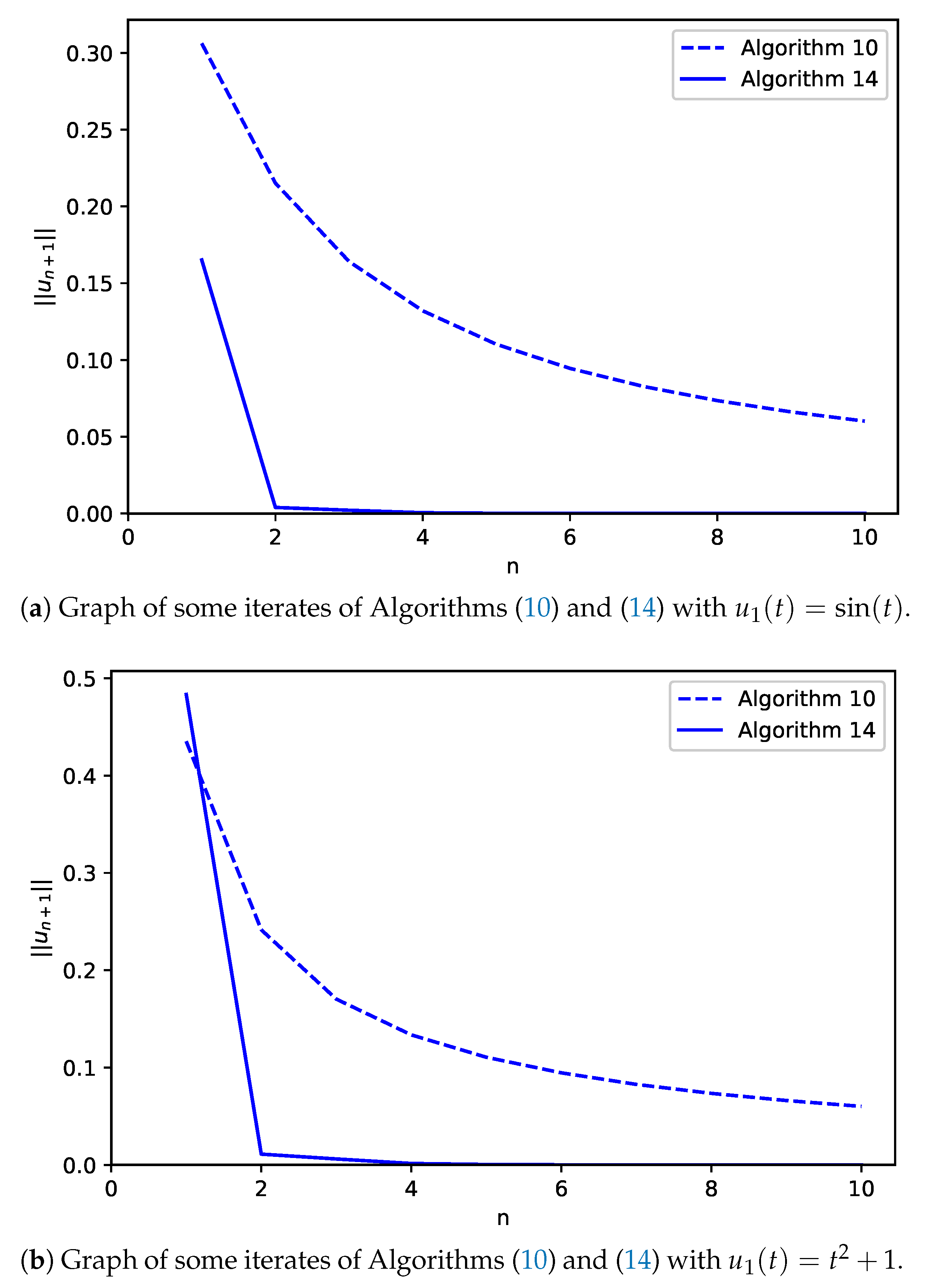
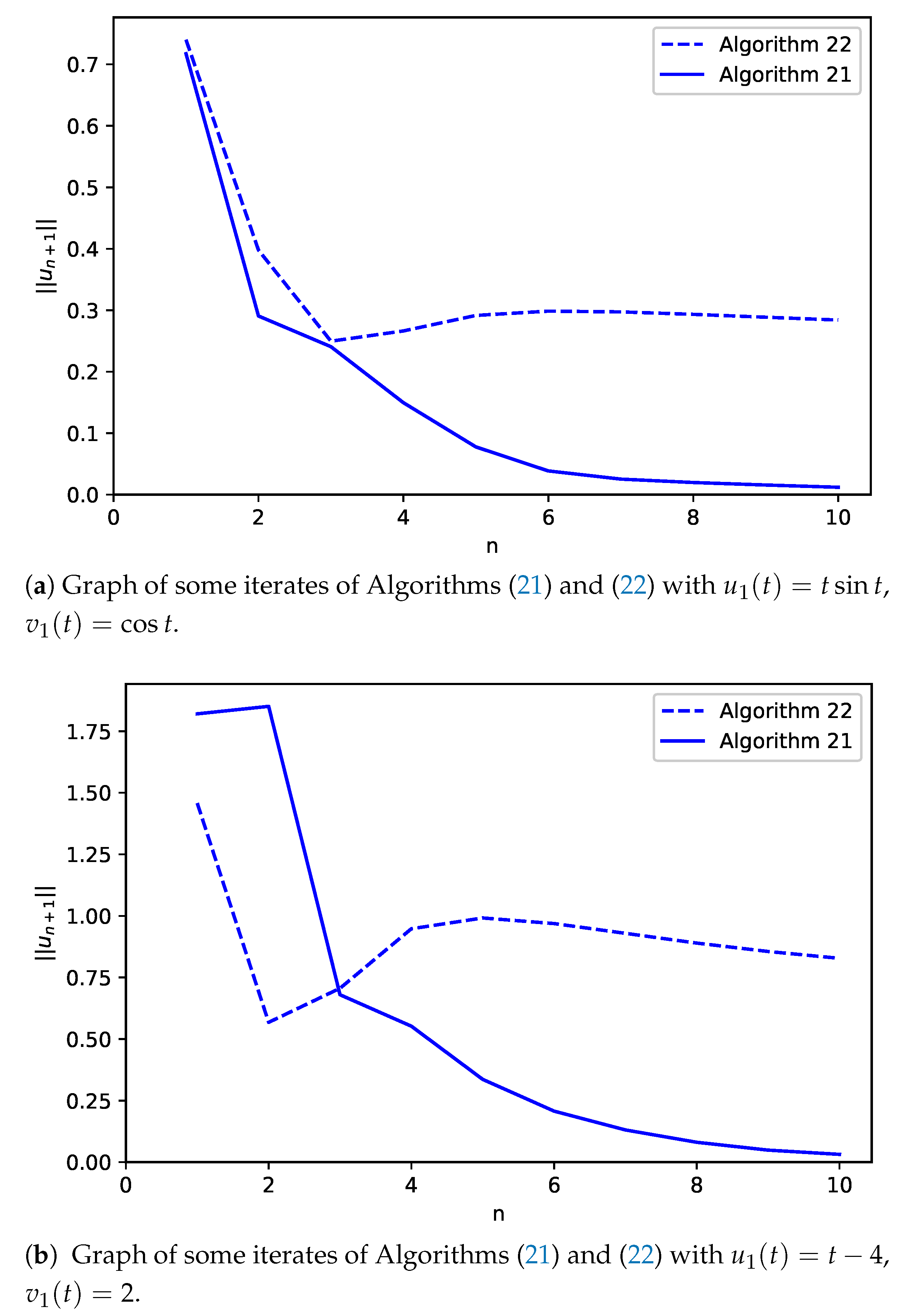
5. Numerical Experiments

In this section, we give comparisons of the numerical performance of our algorithms with the performance of some recent important algorithms.
Example 1. 
(Zeros of m-accretive operator in L 3 ( [ 0 , 1 ] ) , see Table 1 and Figure 1 and Figure 2)
In Theorems 1, 2 and 4, set E = L 3 ( [ 0 , 1 ] ) . Let A : E E be defined by
( A u ) ( t ) : = u ( t ) .
Clearly, A is m-accretive and the function u ( t ) = 0 , t [ 0 , 1 ] is in the solutions set. In Theorem 4, take λ n = 1 ( n + 1 ) 1 2 , θ n = 1 ( n + 1 ) 1 4 , β n = 1 ( n + 1 ) 2 , n = 1 , 2 , , as parameters. Also, in Theorem 1, we take α n = 1 n + 1 and λ n = n , and in Theorem 2, we take α n = 1 n + 1 , β n = 1 4 and λ n = 5 . Obviously, these parameters satisfy the assumptions of the theorems, respectively. Using a tolerance of 10 6 and setting maximum number of iterations n = 10 , we get the following:
Example 2. 
(Solutions of Hammerstein equation in L 3 ( [ 0 , 1 ] ) , see Table 2 and Figure 3)
In Theorems 5 and 6, set E = L 3 ( [ 0 , 1 ] ) . Set F , K : E E
F u ( t ) = t u ( t ) , K v ( t ) = v ( t ) .
Clearly, K and F are m-accretive and u * = ( 0 , 0 ) T is in the solutions set. In Theorem 6, we take λ n = θ n = 1 ( n + 1 ) 1 2 , and in Theorem 5, we take α n = 1 ( n + 1 ) 1 2 , θ n = 1 ( n + 1 ) 1 4 , β n = 1 ( n + 1 ) 2 , n = 1 , 2 , , as our control sequences and fixed u 0 = ( 2 , 1 ) T and v 0 = ( 1 , 1 ) T . Obviously, these sequences satisfy the assumptions of the theorems respectively. Using a tolerance of 10 6 and setting maximum number of iterations n = 10 , we get the following iterates:

6. Conclusions

An inertial algorithm for approximating solutions of nonlinear Hammerstein equations is presented. This algorithm is obtained as a consequence of a new inertial algorithm proposed and studied for approximating zeros of m-accretive operators in uniformly smooth real Banach spaces. Strong convergence theorems are proved. Finally, using test examples, comparisons of the numerical performance of our algorithms with the performance of the algorithms of Theorems 6, 9 and 10 are presented. From the experiments (see Table 1 and Table 2 and Figure 1, Figure 2 and Figure 3) our proposed method appears to be competitive and promising.

Author Contributions

The problem was formulated by C.E.C. and the computations and proofs were done jointly by C.E.C., A.A. and M.O.N. All authors have read and agreed to the published version of the manuscript.

Funding

This research is supported from the African Development Bank (AfDB) Research Grant Funds to AUST.

Conflicts of Interest

The authors declare no conflict of interest.

References

  1. Polyak, B.T. Some methods of speeding up the convergence of iteration method. USSR Comput. Math. Phy. 1964, 4, 1–17. [Google Scholar] [CrossRef]
  2. Browder, F.E. Nonlinear mappings of nonexpansive and accretive-type in Banach spaces. Bull. Am. Math. Soc. 1967, 73, 875–882. [Google Scholar] [CrossRef] [Green Version]
  3. Kato, T. Nonlinear semigroups and evolution equations. J. Math. Soc. Jpn. 1967, 19, 511–520. [Google Scholar] [CrossRef]
  4. Cioranescu, I. Geometry of Banach Spaces, Duality Mappings and Nonlinear Problemss; Kluwer Academic Publisher: Bucharest, Romania, 1990; Volume 62. [Google Scholar]
  5. Barbu, V. Dissipative sets and nonlinear pertubated equations in Banach spaces. Ann. Sc. Norm. Pisa 1972, 26, 365–390. [Google Scholar]
  6. Brezis, H.; Pazy, A. Accretive sets and differential equations in Banach spaces. Israel J. Math. 1970, 8, 367–383. [Google Scholar] [CrossRef]
  7. Martinet, B. Régularisation ďinéquations variationnelles par approximations successives. Rev. Fr. Dinformatique Rech. Opér. 1970, 4, 154–158. [Google Scholar]
  8. Rockafellar, R.T. Monotone operators and the proximal point algorithm. SIAM J. Cont. Optim. 1976, 14, 877–898. [Google Scholar] [CrossRef] [Green Version]
  9. Chidume, C.E.; Adamu, A.; Minjibir, M.S.; Nnyaba, U.V. On the strong convergence of the proximal point algorithm with an application to Hammerstein equations. J. Fixed Point Theory Appl. 2020, 22. [Google Scholar] [CrossRef]
  10. Chidume, C.E.; De Souza, G.S.; Nnyaba, U.V.; Romanus, O.M.; Adamu, A. Approximation of zeros m-accretive mappings, with applications to Hammerstein integral equation. Caparthian J. Math. 2020, 36, 45–55. [Google Scholar]
  11. Xu, H.K. Strong convergence of an iterative method for nonexpansive and accretive operators. J. Math. Anal. Appl. 2006, 314, 631–634. [Google Scholar] [CrossRef]
  12. Qin, S.; Su, Y. Approximation of a zero point of a accretive operator in Banach spaces. J. Math. Anal. Appl. 2007, 329, 415–424. [Google Scholar] [CrossRef]
  13. Chidume, C.E. Strong convergence theorems for bounded accretive operators in uniformly smooth Banach spaces. Contemp. Math. 2016, 659, 31–41. [Google Scholar]
  14. Chidume, C.E.; Djitte, N. Strong convergence thoerems for bounded maximal monotone nonlinear operator U in Hilbert space. Abstr. Appl. Anal. 2012. [Google Scholar] [CrossRef] [Green Version]
  15. Xu, Z.B.; Roach, G.F. Characteristic inequalities of uniformly convex and uniformly smooth Banach space. J. Math. Anal. Appl. 1991, 157, 189–210. [Google Scholar] [CrossRef] [Green Version]
  16. Chidume, C.E. Geometric Properties of Banach Spaces and Nonlinear Iterations; Springer: London, UK, 2009. [Google Scholar]
  17. Xu, H.K. Iterative algorithm for nonlinear operators. J. Lond. Math. Soc. 2000. [Google Scholar] [CrossRef]
  18. Reich, S. Strong convergence theorems for resolvents of accretive operators in Banach spaces. J. Math. Anal. Appl. 1980, 75, 287–292. [Google Scholar] [CrossRef] [Green Version]
  19. Fitzpatrick, P.M.; Hess, P.; Kato, T. Local boundedness of monotone type operators. Proc. Jpn. Acad. 1972, 48, 275–277. [Google Scholar] [CrossRef]
  20. Pascali, D.; Sburian, S. Nonlinear Mappings of Monotone Type; Editura Academia Bucuresti: Bucharest, Romania, 1978. [Google Scholar]
  21. Chidume, C.E.; Adamu, A.; Chinwendu, L.O. Iterative algorithms for solutions of Hammerstein equations in real Banach spaces. Fixed Point Theory Appl. 2020. [Google Scholar] [CrossRef]
  22. Brézis, H.; Browder, F.E. Nonlinear integral equations and systems of Hammerstein type. Bull. Am. Math. Soc. 1976, 82, 115–147. [Google Scholar] [CrossRef] [Green Version]
  23. Browder, F.E.; De Figueiredo, D.G.; Gupta, C.P. Maximal monotone operators and nonlinear integral equations of Hammerstein type. Bull. Am. Math. Soc. 1970, 76, 700–705. [Google Scholar] [CrossRef] [Green Version]
  24. Browder, F.E.; Gupta, C.P. Monotone operators and nonlinear integral equations of Hammerstein type. Bull. Am. Math. Soc. 1969, 75, 1347–1353. [Google Scholar] [CrossRef]
  25. De Figueiredo, D.G.; Gupta, C.P. On the variational methods for the existence of solutions to nonlinear equations of Hammerstein type. Bull. Am. Math. Soc. 1973, 40, 470–476. [Google Scholar]
  26. Chidume, C.E.; Adamu, A.; Chinwendu, L.O. Approximation of solutions of Hammerstein equations with monotone mappings in real Banach spaces. Carpathian J. Math. 2019, 35, 305–316. [Google Scholar]
  27. Chidume, C.E.; Bello, A.U. An iterative algorithm for approximating solutions of Hammerstein equations with monotone maps in Banach spaces. Appl. Math. Comput. 2017, 313, 408–417. [Google Scholar] [CrossRef]
  28. Chidume, C.E.; Nnakwe, M.O.; Adamu, A. A strong convergence theorem for generalized-Φ-strongly monotone maps, with applications. Fixed Point Theory Appl. 2019. [Google Scholar] [CrossRef] [Green Version]
  29. Chidume, C.E.; Zegeye, H. Approximation of solutions of nonlinear equations of Hammerstein type in Hilbert space. Proc. Am. Math. Soc. 2005, 133, 851–858. [Google Scholar] [CrossRef]
  30. Chidume, C.E.; Adamu, A.; Nnakwe, M.O. Strong convergence of an inertial algorithm for maximal monotone inclusions with applications. Fixed Point Theory Appl. 2020. [Google Scholar] [CrossRef]
  31. Chidume, C.E.; Zegeye, H. Approximation of solutions of nonlinear equations of monotone and Hammerstein type. Appl. Anal. 2003, 82, 747–758. [Google Scholar]
  32. Shehu, Y. Strong convergence theorem for integral equations of Hammerstein type in Hilbert spaces. Appl. Math. Comput. 2014, 231, 140–147. [Google Scholar] [CrossRef]
  33. Chidume, C.E.; Zegeye, H. Iterative approximation of solutions of nonlinear equations of Hammerstein type. Abstr. Appl. Anal. 2003, 2003, 353–365. [Google Scholar] [CrossRef] [Green Version]
Figure 1. Graph of some iterates of Algorithms (9) and (14).
Symmetry 13 00376 g001
Figure 2. Graph of some iterates of Algorithms (10) and (14).
Symmetry 13 00376 g002
Figure 3. Graph of some iterates of Algorithms (21) and (22).
Symmetry 13 00376 g003
Table 1. Numerical experiment for Example 1 (for zeros of m-accretive map).
Algorithm (9)Algorithm (10)Algorithm (14)
IPn u n + 1 T (s)IPn u n + 1 T (s)IPn u n + 1 T (s)
u 1 ( t ) = sin t 100.05010.029 u 1 ( t ) = sin t 100.06021.431 u 0 ( t ) = t 103.0630 × 10 6 17.252
u 1 ( t ) = sin t
u 1 ( t ) = t 2 + 1 100.05010.020 u 1 ( t ) = t 2 + 1 100.06020.040 u 0 ( t ) = t 108.887 × 10 6 12.308
u 1 ( t ) = t 2 + 1
u 1 ( t ) = 1 2 t + cos t 100.05010.024 u 1 ( t ) = 1 2 t + cos t 100.06020.062 u 0 ( t ) = t 103.942 × 10 6 19.140
u 1 ( t ) = 1 2 t + cos t
Table 2. Numerical experiment for Example 2 (For Hammerstein equation).
Algorithm (22)Algorithm (21)
IPn u n + 1 T (s)IPn u n + 1 T (s)
u 1 ( t ) = t sin t 100.28410.711 u 1 ( t ) = t sin t 100.0121759.29
v 1 ( t ) = cos t
u 1 ( t ) = t 4 100.82771.564 u 1 ( t ) = t 4 100.0317646.93
v 1 ( t ) = 2
u 1 ( t ) = 4 100.95260.637 u 1 ( t ) = 4 100.145521.39
v 1 ( t ) = e t + 2 t
Publisher’s Note: MDPI stays neutral with regard to jurisdictional claims in published maps and institutional affiliations.

