Abstract
Clustering is a mathematical approach that allows one to find a group of data with similar attributes. This approach is also often used in the field of computer science to group a large amounts of data. Triclustering analysis is an analysis technique on 3D data (observation—attribute—context). Triclustering analysis can group observations on several attributes and contexts simultaneously. Triclustering analysis has been frequently applied to analyze microarray gene expression data. We proposed the -Trimax method to perform triclustering analysis on microarray gene expression data. The -Trimax method aims to find a tricluster that has a mean square residual smaller than and a maximum volume. Tricluster is obtained by deleting nodes from 3D data using multiple node deletion and single node deletion algorithms. The tricluster candidates that have been obtained are checked again by adding some previously deleted nodes using the node addition algorithm. In this research, the program improvement of the -Trimax method was carried out and also the calculation of the resulting tricluster evaluation result. The -Trimax method is implemented in two microarray gene expression data. The first implementation was carried out on gene expression data from the differentiation process of human-induced pluripotent stem cells (HiPSCs) from patients with heart disease, resulting in the best simulation when , , and obtained five tricluster, which are considered as characteristics of heart disease. The second implementation was implemented on HIV-1 data, best simulation when , and produced three genes as biomarkers, with the gene names AGFG1, EGR1 and HLA-C. This gene group can be used by medical experts in providing further treatment.
1. Introduction
The enormous development of data in almost every area of life has generated a great demand for an analytical technique that can turn data into useful knowledge. Efforts to gain knowledge from these data are often referred as data mining [1,2]. As an important research content in data mining and artificial intelligence, clustering is an unsupervised pattern recognition method without prior information guidance (the dataset does not have a column to explain which observation belongs to a particular class or group). It aims to find potential similarities and grouping so that the distance between two points in the same cluster is as small as possible and the distance between data points in different clusters is the opposite [3].
One of the data analysis techniques that are often used to perform data mining is clustering analysis [4,5,6]. The form of data used in clustering is a two-dimensional (2D) data matrix consisting of rows and columns, row dimensions are usually observations and columns are data attributes. Clustering analysis aims to divide a set of observation data into several groups or clusters. Observations of data that are in the same cluster will have similarities and are not similar to observations that are in different clusters [7].
Clustering analysis can only group objects from one data dimension (observations or attributes) separately, so that a data sub-matrix is obtained in the form of a subset of observations by containing all attributes [8,9]. However, for some research problems, there is an urge to find a data sub-matrix in the form of a subset of observations and does not have to contain all attributes. So it must be done by clustering the observations and attributes simultaneously. The data analysis technique that can do this is biclustring analysis. Biclustering analysis can group the two dimensions of data simultaneously, so that further knowledge can be obtained about the problems of the data used [10,11].
Facing increasingly complex data problems, where the data used is not only in two-dimensional form but can be three-dimensional (3D) data, data analysis techniques are developed that can cluster 3 data dimensions simultaneously. This analysis is known as triclustering analysis. For example, 3D data consists of observation dimensions, attributes and context, then by using triclustering analysis, a tricluster can be obtained, which is a sub-space of 3D data. The resulting tricluster is a subset of observations, a subset of conditions and a subset of attributes from 3D data [8,9].
Triclustering analysis is often performed to analyze microarray gene expression data. Microarray is a technology that can be used to measure the level of thousands genes expression under several conditions simultaneously. Microarray technology can also observe gene expression at a certain time, resulting in 3D data on gene expression [12]. 3D data on microarray gene expression usually consists of gene dimensions, conditions, and time points of observation. The purpose of conducting triclustering analysis on microarray gene expression data is to find groups of genes that have similar expressions in a subset of conditions as well as a subset of observation time points [12].
The triclustering method for analyzing 3D gene expression data was first proposed by [13] under the name Tricluster. After [13] proposed the triclustering analysis method, many researchers proposed various new methods for analyzing 3D data. In 2007, Ref. [14] proposed the Extended Dimension Iterative Signature Algorithm (EDISA) method that can be used when the data re unbalanced, where the number of points of observation time is not the same in each experimental condition. [15] proposed an OPTricluster algorithm that can maintain the time sequence in gene expression data. OPTricluster is effectively used to analyze short time series data (3–5 time points) and has 2–5 experimental conditions [15].
One of the triclustering methods used to analyze microarray gene expression data is the -Trimax method. The -Trimax method can produce a sub-space or tricluster that has a mean square residual smaller than [12]. The -Trimax method can be used for gene expression data that has many conditions and time points (long time series) in an experiment. In this paper, the -Trimax program is created using the Python programming language, which is an improvement in calculating multiple node deletion and node addition. This program also adds a calculated evaluation of each tricluster found. This is a novelty of the program that was previously made by [16]. Program can be accessed on https://github.com/novalsaputra/Delta-Trimax (accessed on 18 January 2021).
The implementation of the -Trimax method was carried out on microarray gene expression data from the differentiation process of human induced pluripotent stem cell (HiPSC) in patients with heart disease and HIV-1. This data were obtained from the web page “www.ncbi.nlm.nih.gov”. The expected result of this study is the discovery of gene groups that have similar expressions in the condition subset and the observation time point subset. The acquired gene group can be used as a guide by medical and biologists to carry out further action on patients.
This paper mainly discusses the triclustering method used in gene expression data in a microarray format. We see a match between our topics with the mathematics and computer science scope in the journal Symmetry, especially in transformation (matrix transformation), pattern recognition (unsupervised learning), diversity, and similarity. Therefore, we choose symmetry journal as the venue of our research work. We also cited one research within the symmetry journal to deepen our knowledge of the most recent research on the published clustering research (although it does not necessarily using the same dataset and the same data dimension compared to this paper).
2. Theoretical Basis
2.1. Perfect Shifting Clustering
Perfect shifting triclustering represents the estimated value for each subspace element that is a tricluster. Suppose that the subspace with and , then is said to be perfect shifting triclustering when each element in that can be represented as given in Equation (1):
where is a constant value for tricluster, is the effect of the ith observation , is the effect of the jth attribute and, is the effect of the kth context . To obtain Equation (1), first, the average element value for each node is calculated, and the average value of the overall elements in the matrix . Node is a term for the dimensional member in 3D datasets. Suppose is the number of objects in the set and K. Here is an equation for calculating the average at each node.
Equation (2) calculates the average value for the ith observation, Equation (3) calculates the average value of the jth attribute, and Equation (4) calculates the average value for the kth context or time. The average of the total elements in the tricluster is presented in Equation (4).
The effect of each node in the tricluster is obtained by calculating the difference between the mean of each node and its total mean.
2.2. Mean Squared Residual
The residual value is obtained by comparing the original value of the data element with its estimated value. The estimated value for each element in the tricluster is obtained through the perfect shifting triclustering value of the data element. By using Equation (9), the residual value for each tricluster data element is obtained using Equation (10):
When mean square residual obtained on the tricluster approaches 0, this indicates that the tricluster has high homogeneity [8].
2.3. Triclustering Quality Index (TQI)
Triclustering Quality Index (TQI) is the score used to evaluate the tricluster generated in the triclustering analysis. is defined in Equation (12):
where is the mean square residual in the ith tricluster, is the number of observations in the ith tricluster, is the number of attributes in the ith tricluster, is the number of contexts in the ith tricluster. The research conducted by [17] states that the tricluster, which has a small TQI value, presents a tricluster with good quality. This means that the tricluster will have good quality when the data in the tricluster has a high homogeneity (when the mean square residual is small) and also has many data elements (large volume).
3. Methodology
The method used to perform triclustering in this study is the -Trimax method. 3D data in this method is focused on the problem of microarray gene expression, where the data consists of the dimensions of genes (observation), conditions (attributes), and time (context). The -Trimax method is a greedy approach that uses an iteration search scheme, where objects are gradually added and removed from the candidate subspace tricluster to meet certain criteria. This method aims to find a tricluster that has a mean square residual (S) smaller than . is the threshold determined based on the perspective of the researcher. The -Trimax method is composed of several algorithms, namely the multiple node deletion algorithm, the single node deletion algorithm and the node addition algorithm. As the name implies, these algorithms perform iteration deletions and additions of nodes, resulting in a tricluster that has a mean square residual smaller than . Then the tricluster that has been found is masked so that other triclusers can be found in the 3D data. The workflow of the -Trimax method in this study is shown in Figure 1.
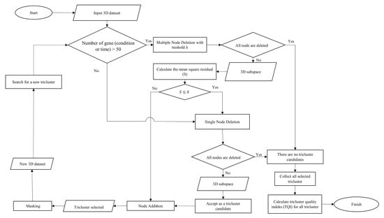
Figure 1.
Flowchart of the -Trimax algorithm.
3.1. Multiple Node Deletion Algorithm
The multiple node deletion algorithm performs the deletion of nodes which are thought to increase the mean square residual S. The number of nodes that are removed in each iteration is large or equal to one. This algorithm determines a value of which is used as the threshold to control the number of deletions performed. The value of can be adjusted experimentally to optimize the speed of the algorithm. When the number of genes, conditions or times in the data is less than 50, then this algorithm is not executed on the data [12]. This is to avoid the algorithm deleting all nodes in small 3D data. The purpose of this algorithm is that the data sub-space found does not have an S value that is too far from the predetermined , to save the computation process for the next step.
Here are the steps of the multiple node deletion algorithm on the matrix :
- When then proceed to step 2, otherwise the process is not continued and gives as the final result of this algorithm.
- Delete the ith gene if it satisfies the following inequality:.
- Recalculate:and S.
- Delete the jth condition if it satisfies the following inequality:.
- Recalculate:and S.
- Repeat step 2 to step 7. If there are no genes, conditions and times are deleted then the iteration stops.
The complexity of this algorithm is O(max(m,n,p)) where m,n and p are the number of genes, conditions and time-points [12].
3.2. Single Node Deletion Algorithm
The single node deletion algorithm performs deletion of nodes iteratively until the S generated by the data sub-space has a value small or equal to the threshold . The single node deletion algorithm only deletes one node in each iteration, so the computation time at this step is quite long. Therefore, before running the single node deletion algorithm, the multiple node deletion algorithm is first to run.
Following are steps of the single node deletion algorithm:
- Detect the gene, condition, and time that has the highest residual score in the following way:
- The residual score for the ith gene, :
- The residual score for the jth condition, :
- The residual score for the kth time, :
- Delete the gene, condition or time that has the highest score.
- Recalculate and S.
- Repeat step 1 to step 3. If value then iteration stops.The final result of the single node deletion algorithm is subspace which has a value of , where and .
The complexity of this algorithm is O(log m + log n + log p) where m,n and p are the number of genes, conditions and time-points [12].
3.3. Node Addition Algorithm
The -Trimax method aims to find the tricluster which has a maximum volume and a small mean square residual (S) of the threshold . In the single node deletion algorithm, a tricluster has been obtained which has . However, this tricluster may not be the tricluster with the maximum volume that can be extracted from 3D dataset, therefore it is necessary to double check the previously deleted nodes. Checking is done by adding nodes that are not members of the tricluster (nodes that were deleted previously) on the condition that the value of S remains small from . The following are the steps for the addition node algorithm:
- Add genes that satisfy
- Recalculate and S.
- Add conditions that satisfy.
- Recalculate and S.
- Add times that satisfy.
- Recalculate and S.
- Repeat step 1 to step 6. If there are no more nodes added to the gene, condition and time then the iteration stops.
The final result of node addition algorithm is a subspace , where , and . The data sub-space generated by this algorithm is a tricluster with and has a maximum volume. The complexity of this algorithm is O(mnp) as each iterates (m+n+p) times [12].
3.4. Algorithm Simulation
This chapter aims to simulate triclustering discovery using the proposed -trimax algorithm using a small sample of data, as given in Table 1. The steps in this simulation are based on Figure 1. The dataset in Table 1 consists of 5 genes, three conditions, and 4-time steps. Before employing -trimax algorithm, a threshold value for both and are required. In this simulation, we initialize and , when using real data, and can be obtained in discussion 4.2. According to Table 1, we know that the total number of genes, condition, and time steps are less than 50, so we don’t need to perform multiple node deletion and apply single node deletion directly. This steps initialized by calculating and S using Equations (2)–(4) and (11) respectively.

Table 1.
Gene expression dataset example.
3.4.1. Precomputing
Assume that I is the set of genes, J is the set of conditions, and K is the set of time steps. According to Table 1, and . The calculations of are given as follows:
The calculations of are given as follows:
The calculations of are given as follows:
The calculation of is given as follows:
By using using the values that have been obtained above, we can get residual value for each element within dataset using Equation (10). For example, for element (, and ):
By counting residual value for each element on each datum, we have got the residual value calculation result, as given in Table 2.
Table 2.
Residual value for each datum.
3.4.2. Single Node Deletion
We will calculate single node deletion through four following iterations:
- Iteration 1The single node deletion algorithm computes residual score on each gene, condition and time step using residual data in Table 2.
- Residual score at .Based on the calculation above, we’ve got as the highest gene residual score which yield .
- Residual score calculation where :Based on the calculation above, the residual score obtained at in the amount of .
- Residual score calculation for :
Table 3 summarizes residual scores on genes, conditions, and time steps for iteration 1.
Table 3. Residual score summarization for iteration 1.Based on Table 3 on all columns, we’ve got 54.37 as the highest score. This highest score is obtained on , so that makes erased. The sets condition after the first iteration are , , and . After the deletion is done, check again whether the S value on sub-space is smaller than . In order to do that, we need to recalculate and S on the current sets.Using the same way as before, we have got the average value for each gene, condition and time step as follows:We use the values obtained in Table 4 to find the value for S using Equation (11). We got . Because of then the node deletion is done again for the next iteration using data given in Table 5.
Table 4. The Average of Each Gene, Condition, and Time Step for Iteration 1.
Table 5. Single node deletion result on iteration 1. - Iteration 2Table 6 summarizes residual scores on genes, conditions, and time steps for iteration 2.
Table 6. Residual score summarization for iteration 2.The maximum score based on Table 6 is 50.43, so the removed from the data. The new data obtained after node deletion consists of and . We compute and S of the current data.According to Table 7, and , because of then the node deletion is done again for the next iteration using data given in Table 5. Table 8 summarizes residual scores on gene , condition , and time step for iteration 2.
Table 7. The average of each gene, condition, and time step.
Table 8. Single node deletion result on iteration 2.
- Iteration 3Table 9 summarizes residual scores on gene , condition , and time step for iteration 3. The maximum score obtained at which equal to 39.19. Therefore, we remove on the dataset and recalculate and S. The current dataset are , and . The same calculation steps are carried out and we got which is bigger than . Therefore the calculation is repeated again on iteration 4.
Table 9. Residual score summarization.
- Iteration 4According to Table 10, we have got . Because , iteration for single node deletion is terminated. The next step is to perform a node addition algorithm using the data in Table 11. Table 12 summarizes residual scores on gene , condition , and time step for iteration 3.
Table 10. The average of each gene, condition, and time step for iteration 4.
Table 11. Single node deletion result on iteration 4.
Table 12. Residual score summarization for iteration 4.
3.4.3. Node Addition Algorithm
We will add genes, conditions, and time steps to keep the S value smaller than the value. The data used are given in Table 11 where and . The mean values for each gene, condition, time step and S for the data in Table 11 were previously obtained, so there was no need to recount those values.
- Gene addition toCalculate for :Residual score for gene calculation:According to Table 13, we obtained and , these values bigger than , then no new datum is added to the dataset.
Table 13. Node addition data (gene on ).
- Condition addition toCalculates for :Residual score for condition :According to Table 14 , then no new datum is added to the dataset.
Table 14. Condition addition data (condition on ).
- Time step addition forCalculates for :Residual score for condition :According to Table 15, we obtained, , then no new time steps are added to the data in Table 11. From the addition node algorithm results, it turns out that there is no addition to genes, conditions, and time, so the algorithm is stopped and not continued to the next iteration. Because there are no additional nodes, the data for this algorithm’s final result is the same as the initial data used (as given in Table 11).
Table 15. Time step addition data (time step on ).The final result produced by addition node algorithm is a tricluster obtained from the first iteration of the -Trimax method. Therefore, the data in Table 11 is a tricluster that has sub-space with , , and .
3.4.4. Masking
According to the calculation of node deletion and node addition, one tricluster has been obtained in Table 1. The resulting tricluster is the data shown in Table 11. To find another tricluster, the data element containing the tricluster in Table 1 are exchanged with random numbers. Since the tricluster obtained previously is a data sub-space with , and , the data elements that are exchanged are elements that are members .
After the masking process has been carried out, the next step is to repeat the -Trimax method using the 3D data in Table 11, so that a new tricluster can be found. The tricluster search stops when no tricluster is found in data that has ; this condition will stop the search iteration for the -Trimax method. The numbers in bold in Table 16 are the datum that has been masked.
Table 16.
Masking process result data.
4. Implementation Results
4.1. The Dataset
The implementation was carried out on two types of microarray gene expression data. The first gene expression data were obtained from the official NCBI website (https://www.ncbi.nlm.nih.gov/geo/query/acc.cgi?acc=GSE35671 accessed on 2 January 2020). The data contains the level of gene expression during the differentiation process of human induced pluripotent stem cell (HiPSC) in genes of patients with heart disease. HiPSC differentiation is a process that can repair and replace genes from damaged samples. By observing gene expression during this process can provide an understanding of the molecular events of gene changes in the human body [12]. The resulting microarray gene expression data consisted of 48,803 genes. This observation was carried out for three replications. At each replication, gene expression was measured at the same 12 time points. Time point is the time of observation on days 0, 3, 7, 10, 14, 20, 28, 35, 45, 60, 90 and 120. Day 0 is the expression of the initial genes of heart disease before differentiation.
The second gene expression data were obtained from the following ncbi web page (https://www.ncbi.nlm.nih.gov/geo/query/acc.cgi?acc=GSE6740 accessed on 7 November 2020). The data were the expression of the HIV-1 gene consisting of 22,283 idea probes, 40 observations from four conditions. The 40 observations consisted of 10 observations that had normal conditions, 10 observations that had acute conditions, 10 observations that had chronic conditions, and 10 observations that had non-progressor conditions. HIV is a virus that causes many deaths in the world. HIV infects and destroys an important part of the immune system to fight infection, namely CD4+ cells which are a type of white blood cell. The more CD4+ cells that are destroyed make the body more susceptible to various kinds of diseases and infections. HIV can be classified into two main types, namely HIV-1 and HIV-2. Patients infected with HIV-2 generally have a higher survival after experiencing a series of HIV symptoms. Meanwhile, HIV-1 is a deadly disease that requires immediate treatment during infection [18].
One of the aims of this experiment is to determine the relationship between genes in gene expression microarray data. From previous research, the relationship between genes can be obtained by clustering genes. For gene expression of heart disease, can be obtained a group of genes that are suspected of causing heart disease. To find out at any time the genes have similar expressions, clustering can be done to the point of observation time. Furthermore, replication in the experiment is used to obtain more valid gene expression readings from the microarray tool, this has often been done by other researchers. By clustering this replication, it is possible to obtain replication clusters that produce data that tend to be similar. So that this clustered replication is a replication that results in more valid gene expression data because it produces similar gene expression values in each experiment [19]. Instead of grouping genes, conditions, and time separately, we can use triclustering techniques to get groups of genes that also cluster at replication and time. Likewise for HIV-1 data, using the triclustering technique, gene groups can be obtained by grouping together genes, conditions, and observations.
4.2. Determination of Threshold and
The value for depends on the distribution of values in the data used, so each data can have a different value of . Therefore, to obtain guidelines in determining , according to [12] the following steps can be taken:
- In each condition, gene clustering was performed against time using the K-Means method.
- For each cluster generated from stage 1, time clustering was carried out on genes using the K-Means method.
- Each cluster produced in stage 2 is calculated the mean square residual (S) value. The smallest S is used as .
This study selected the five smallest mean square residuals (S) from the resulting cluster as which consisted of and . Next was the determination of the value of which was used as a threshold in the multiple node deletion algorithm. In this implementation, three lambda thresholds were used, namely and .
4.3. Simulation Comparison
The best simulation was obtained by comparing the average TQI () values. The simulation was also compared based on the computation time to find the tricluster.
Based on the graph in Figure 2, it can be seen that the greater and used, the value () obtained tended to be higher. Best simulation was obtained when () was small. From the graph, it can be seen that () the smallest value obtained when using and .
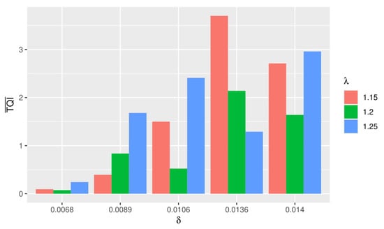
Figure 2.
Comparison graph of Triclustering Quality Index (TQI) and computation time in each simulation.
Thus it can be concluded that the best simulation was obtained when using and . Based on Figure 2, it was found that the greater the value of given, the longer the computation time was. This was inversely proportional to the value of, the greater it was, the faster the computation time tended to be.
5. Discussion
5.1. HiPSC Triclustering Performance
Based on Figure 2, the best -Trimax simulation was obtained when using the threshold and with a computation time of 162.64 min. The number of tricluster obtained from the simulation was 302 tricluster. Here are 10 triclusters that had the smallest TQI. If look at the 10 triclusters in Table 5, triclusters 1, 2, 4, 7, 9 are clustered in all replications (three replications) while the triclusters 3, 5, 6, 8, 10 are only clustered in two replications. This indicates that each tricluster obtained was not clustered in all replication experiments. This means that there were several readings of different gene expression values for each replication, even though it was measured at the same time. When considering multiple replications to determine clusters of gene expression, the resulting gene pool results were also more valid.
If the value of delta and lambda is bigger, the computation time will be longer (Figure 3 and Figure 4). The HiPSC differentiation process is often used to determine which gene group causes a disease, therefore this gene group can be used as a target for therapy or to be used in developing treatment drugs. From the resulting tricluster, we can get a group of genes that are thought to cause heart disease, thus gene groups can be treated. In addition to getting the gene group that will be the target of therapy, the use of a tricluster can predict the point in time when the therapy should be done. In Table 17, there are time points grouped on each tricluster. The point in time inside the tricluster is marked (X).
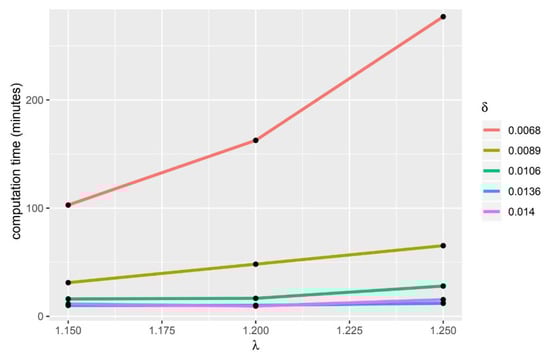
Figure 3.
usage comparison.
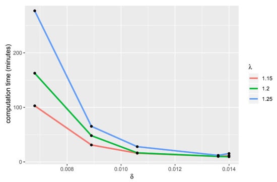
Figure 4.
usage comparison.
Table 17.
List of 10 triclusters with smaller TQI.
5.2. HIV-1 Triclustering Performance
The discovery of the tricluster was carried out using the -Trimax method by performing 15 simulations with different and . Figure 5 illustrates the average obtained for each TQI.
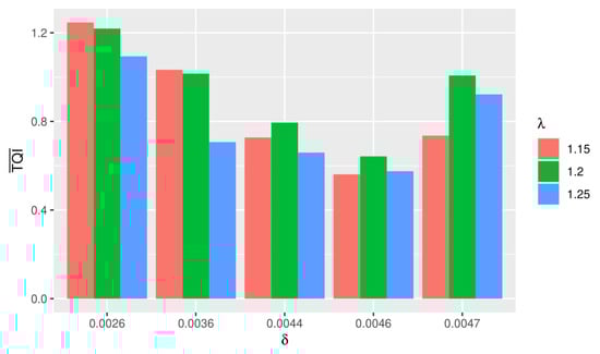
Figure 5.
Average obtained for each TQI.
The best simulation was obtained when and proceeded with a computation time of 20.04 minutes. From this simulation, 202 triclusters were obtained, then we selected 10 triclusters with the smallest TQI. The selected tricluster was validated with a GeneCard on the GPL96 platform downloaded on NCBI. Validation aimed to determine the name of the gene associated with HIV-1 based on the probe ID obtained. According to Table 18, the tricluster with HIV-1 genes associated was obtained, namely AGFG1, EGR1, and HLA-C. Research conducted by [10] can further prove the results obtained in this study.
Table 18.
The 10 selected triclusters along with genes associated with HIV-1
5.3. DNA/RNA Sequences
Research conducted by [5,11] revealed that the clustering method could be done on DNA sequence data. According to [5], this clustering method is used to identify virus groups and analyze relationships between these virus groups. Clustering itself is a method that flexible in its implementation. [5] encourages readers to implement the k-mer sparse matrix for hierarchical clustering using a different metric distance. Moreover, readers could apply the method that they use to analyze other biological data to conduct comparative studies against other clustering methods.
Although the method we propose is implemented on microarray data, our method can also be implemented on other data (e.g., RNA-Seq) as long as the data is three-dimensional. The research conducted by [20] implements 3D clustering using RNA sequence data. The data they use is pan-cancer epigenetic data downloaded from the website of the NIH Roadmap Epigenome Project. Epigenetic alteration is a fundamental characteristic of nearly all human cancers. Tumor cells not only harbor genetic alterations but also are regulated by various epigenetic modifications. Identification of epigenetic similarities across different cancer types is beneficial for discovering treatments that can be extended to different cancers. [20] proposed a new approach TriPCE, introducing a tri-clustering strategy to integrative pan-cancer epigenomic analysis. The method is able to identify coherent patterns of various epigenetic modifications across different cancer types. To validate its capability, the authors [20] applied the proposed TriPCE to analyze six important epigenetic marks among seven cancer types and identified significant cross-cancer epigenetic similarities. These results suggest that specific epigenetic patterns indeed exist among these investigated cancers. Furthermore, the functional gene analysis performed on the associated gene sets demonstrates strong relevance with cancer development and reveals consistent risk tendency among these investigated cancer types.
The microarray data format is considered an outdated data format. Microarrays are reliable and more cost-effective than RNA-Seq for gene expression profiling in model organisms. RNA-Seq will eventually be used more routinely than microarray, but right now, the techniques can be complementary to each other. Microarrays will not become obsolete but might be relegated to only a few uses [21].
6. Conclusions
The -Trimax method form triclusters from 3D data which has a large dimension level. Our proposed method can be used when the data has many points in time (long time series). The -Trimax method can produce a tricluster that has a smaller mean square residual than the threshold , where the mean square residual is an indicator of the homogeneity of a tricluster. The authors has created a new program for analyzing 3D data using the -Trimax method. The novelty of the program is improvements in calculating the multiple node deletion, node additions algorithm and evaluation algorithm for each generated tricluster.
The implementation of the -Trimax method was carried out on gene expression data from the HiPSC differentiation process in patients with heart disease and HIV-1. From the results of the implementation, the following conclusions were obtained:
- From several simulations using different and , the best simulation is obtained when using and for HiPSC, and for HIV-1.
- The best five tricluster based on the smallest TQI for HiPSC data. This group of gene expression within the five tricluster is thought to be a feature of heart disease. Therefore, this gene group can be used by medical experts in providing further treatment, such as making the genes in this tricluster a therapeutic target or as a drug development.
- Three biomarkers for HIV-1 disease were obtained from the 10 selected tricluster. Biomarkers consist of genes AGFG1, EGR1, and HLA-C.
Further research include conducting gene ontology analysis (GO) to see the relationship between genes based on their biological characteristics. Furthermore, we can use parallel computing to speed up the computation time in the -Trimax method.
Author Contributions
Conceptualization, T.S.; methodology, N.S. and H.S.A.-A.; software, N.S.; validation; formal analysis, D.S. All authors have read and agreed to the published version of the manuscript.
Funding
This work was fully funded by PUTIQ2 2020 with the contract no. NKB-2827/UN2.RST/ HKP.05.00/2020 from Universitas Indonesia.
Institutional Review Board Statement
Not applicable.
Informed Consent Statement
Not applicable.
Data Availability Statement
The data presented in this study are openly available in the link provided in Section 4.1.
Acknowledgments
NKB-1655/UN2.RST/HKP.05.00/2020 is the number of research grant funding by the Universitas Indonesia for this research. We want to thank you for the research grants to the Universitas Indonesia.
Conflicts of Interest
The authors declare no conflict of interest.
References
- Siswantining, T. Geoinformatics of Tuberculosis (TB) Disease in Jakarta City Indonesia. Int. J. GEOMATE 2020, 19. [Google Scholar] [CrossRef]
- Wibawa, N.A.; Bustamam, A.; Siswantining, T. Differential gene co-expression network using BicMix. AIP Conf. Proc. 2019. [Google Scholar] [CrossRef]
- Lv, Y.; Liu, M.; Xiang, Y. Fast Searching Density Peak Clustering Algorithm Based on Shared Nearest Neighbor and Adaptive Clustering Center. Symmetry 2020, 12, 2014. [Google Scholar] [CrossRef]
- Siswantining, T.; Wulandari, S.; Bustamam, A. Collaboration and implementation of self organizing maps (SOM) partitioning algorithm in HOPACH clustering method. AIP Conf. Proc. 2018, 2014, 020134. [Google Scholar]
- Bustamam, A.; Ulul, E.D.; Hura, H.F.A.; Siswantining, T. Implementation of hierarchical clustering using k-mer sparse matrix to analyze MERS–CoV genetic relationship. AIP Conf. Proc. 2017, 1862, 030142. [Google Scholar]
- Ardaneswari, G.; Bustamam, A.; Siswantining, T. Implementation of parallel k-means algorithm for two-phase method biclustering in Carcinoma tumor gene expression data. AIP Conf. Proc. 2017, 1825, 020004. [Google Scholar]
- Sumathi, S. Introduction to Data Mining and Its Application; Springer: Berlin, Germany, 2006. [Google Scholar]
- Henriques, R. Triclustering Algorithms for Three-Dimensional Data Analysis: A Comprehensive Survey. ACM Comput. Surv. 2018, 51, 95. [Google Scholar] [CrossRef]
- Siska, D.; Sarwinda, D.; Siswantining, T.; Soemartojo, S.M. Triclustering Algorithm for 3D Gene Expression Data Analysis using Order Preserving Triclustering (OPTricluster). In Proceedings of the 2020 4th International Conference on Informatics and Computational Sciences (ICICoS), Semarang, Indonesia, 10–11 November 2020; pp. 1–6. [Google Scholar]
- Kasim, A.; Shkedy, Z.; Kaiser, S.; Hochreiter, S.; Tallon, W. Applied Biclustering Methods for Big and High-Dimensional Data Using R; Taylor & Francis: Boca Raton, FL, USA, 2017. [Google Scholar]
- Sari, I.M.; Soemartojo, S.M.; Siswantining, T.; Sarwinda, D. Mining Biological Information from 3D Medulloblastoma Cancerous Gene Expression Data Using Times Vector Triclustering Method. In Proceedings of the 2020 4th International Conference on Informatics and Computational Sciences (ICICoS), Semarang, Indonesia, 10–11 November 2020; pp. 1–6. [Google Scholar]
- Bhar, A.; Haubrock, M.; Mukhopadhyay, A.; Maulik, U.; Bandyopadhyay, S.; Wingender, E. Extracting Triclusters and Analysing Coregulation in Time Series Gene Expression Data. WABI 2012 LNBI 2012, 2012, 165–177. [Google Scholar]
- Zhao, L.; Zaki, M.J. TRICLUSTER: An Effective Algorithm for Mining Coherent Clusters in 3D Microarray Data. In Proceedings of the 2005 ACM SIGMOD International Conference on Management of Data, Baltimore, MD, USA, 14–16 June 2005; pp. 694–705. [Google Scholar]
- Supper, J.; Strauch, M.; Wanke, D.; Harter, K.; Zell, A. EDISA: Extracting biclusters from multiple time-series of gene expression profiles. BMC Bioinform. 2007, 8. [Google Scholar] [CrossRef]
- Tchagang, A.B.; Phan, S.; Famili, F.; Shearer, H.; Fobert, P.; Huang, Y.; Zou, J.; Huang, D.; Cutler, A.; Liu, Z.; et al. Mining biological information from 3D short time-series gene expression data: The OPTricluster algorithm. BMC Bioinform. 2012, 13, 54. [Google Scholar] [CrossRef]
- Sdraka, M.A. 3D Classification of Gene Expression Data with Use of Machine Learning Methodologies: Cromosomal Classification in Two Stages 2016. National Technical University of Athens. Available online: https://dspace.lib.ntua.gr/xmlui/handle/123456789/43067 (accessed on 10 December 2019).
- Swathypriyadharsini, P.; Premalata, K. TrioCuckoo: A Multi Objective Cuckoo Search Algorithm for Triclustering Microarray Gene Expression Data. J. Inf. Sci. Eng. 2016, 32, 1617–1631. [Google Scholar]
- Trkola, A. HIV–host interactions: Vital to the virus and key to its inhibition. Curr. Opin. Microbiol. 2004, 7, 407–411. [Google Scholar] [CrossRef]
- Bhar, A.; Haubrock, M.; Mukhopadhyay, A.; Wingender, E. Multiobjective Triclustering of Time-Series Transcriptome Data Reveals Key Genes of Bilogical Processes. BMC Bioinform. 2015, 15, 200. [Google Scholar]
- Gan, Y.; Li, N.; Xin, Y.; Zou, G. TriPCE: A Novel Tri-Clustering Algorithm for Identifying Pan-Cancer Epigenetic Patterns. Front. Genet. 2020, 10. [Google Scholar] [CrossRef]
- Stefano, G.B. Comparing Bioinformatic Gene Expression Profiling Methods: Microarray and RNA-Seq. Med Sci. Monit. Basic Res. 2014, 20, 138–142. [Google Scholar] [CrossRef] [PubMed]


Publisher’s Note: MDPI stays neutral with regard to jurisdictional claims in published maps and institutional affiliations. |
© 2021 by the authors. Licensee MDPI, Basel, Switzerland. This article is an open access article distributed under the terms and conditions of the Creative Commons Attribution (CC BY) license (http://creativecommons.org/licenses/by/4.0/).