Abstract
Atomic cascades are ubiquitous in nature and they have been explored within very different scenarios, from precision measurements to the modeling of astrophysical spectra, and up to the radiation damage in biological matter. However, up to the present, a quantitative analysis of these cascades often failed because of their inherent complexity. Apart from utilizing the rotational symmetry of atoms and a proper distinction of different physical schemes, a hierarchy of useful approaches is therefore needed in order to keep cascade computations feasible. We here suggest a classification of atomic cascades and demonstrate how they can be modeled within the framework of the Jena Atomic Calculator. As an example, we shall compute within a configuration-average approach the stepwise decay cascade of atomic magnesium, following a inner-shell ionization, and simulate the corresponding (final) ion distribution. Our classification of physical scenarios (schemes) and the hierarchy of computational approaches are both flexible to further refinements as well as to complex shell structures of the atoms and ions, for which the excitation and decay dynamics need to be modeled in good detail.
1. Introduction
If atoms or ions are initially excited into the continuum of the next higher (or even several times higher) charge state, they often stabilize via various processes towards different ground configurations. Experimentally, this stabilization then results into different spectra (or distributions) of ions, electrons, or photons that need to be understood with regard to their relative intensities, time scales, or even for the coincidence of different events [1,2,3,4]. From a slightly different viewpoint, an atomic cascade typically includes ions of some element in three or more subsequent charge states, and that are connected to each other by different atomic processes, such as (auto-) ionization or photon emission. However, apart from these atomic decay processes, one often also needs to account for the initial excitation and, then, to distinguish between different to distinguish between different cascade schemes, including the photoexcitation and ionization, electron-impact excitation, a (stepwise) decay, or electron-capture cascades [5,6,7,8].
Indeed, numerous investigations in physics, astronomy, and elsewhere are known to be (strongly) affected by atomic cascades. Well-known examples range from the spectroscopy of few-electron ions [9,10] to the study of inner-shell phenomena [11], the diagnostics of plasmas [12,13], the interpretation of astrophysical spectra [14,15], and up to the chemical evolution of the universe [16]. In astrophysics, for example, a current goal refers to a detailed understanding of light curves that help to resolve the chemical evolution of the early universe and, eventually, the formation and growth of galaxies and other structures [17].
However, in practice, (atomic) cascades can exhibit an enormous complexity, even if only the dominant decay pathes are to be considered [18,19,20]. This complexity arises first of all from the large number of decay paths, whose relative importance has been found difficult to estimate in advance. To systematically model such cascades, we make use of Jac, the Jena Atomic Calculator [21] that supports the calculation of different atomic shell structures and processes. The Jac toolbox [22] is based on the concept of many-electron amplitudes and it supports atomic (structure) calculations of different kind and complexity.
In this work, we propose a classification of atomic cascades and shall discuss, in detail, how they can be modeled within the framework of Jac. To this end, we first re-visit the dynamics of (atomic) inner-shell transitions in the next section and emphasize the role of many-electron amplitudes [23,24]. Here, we shall also introduce a few further building blocks that are needed in order to model such cascades. In Section 2, these building blocks then help to distinguish between different cascades schemes, and to account for the initial excitation of the atoms or ions as well as between different cascade approaches. A first implementation within the framework of Jac is outlined and discussed in Section 4, including the stepwise decay of atomic magnesium after K-shell ionization as a rather simple, but non-trivial, example. Apart from the set-up of a cascade model and the computation of all the decay pathes (cascade computations), we also explain how cascade simulations can be carried out in order to extract the requested spectra and information. Finally, in Section 5 we summarize our systematic account and implementation in dealing with atomic cascades. In particular, we hope that this classification will pave the way towards new applications as well as the numerical treatment of complex cascades.
2. Inner-Shell Transitions Revisited
2.1. Following Atomic Decay Lines Basic Notations
Atoms or ions with inner-shell holes usually emit (Auger) electrons and/or photons of certain energies, and that can be observed as—electron or light—spectra by different spectroscopic and detector set-ups. For instance, much of the information that we have about distant stars and many other astrophysical objects originate from the photon emission of particular atoms or molecules at a well-defined wavelength, and that then help to reveal the chemical composition of these objects [25,26]. However, owing to the large number of atomic transitions very rich line spectra have been found in different frequency regions and need to be understood in quite detail in order to analyze astrophysical observations.
At the atomic scale, many of these observations can be perceived within the atomic shell model, and by just taking the level structure into account due to the coupling of electrons. In the shell model, the occupation of (sub-) shells is normally described in terms of electron configurations, such as for the ground configuration of atomic magnesium and magnesium-like ions. Indeed, the use of these (electron) configurations is very crucial to make atomic cascades computable and to extract the requested information about them [27,28]. Each configuration generally comprises (one or) several levels that can be temporarely occupied by a cascade owing to different fine-structure transitions, i.e., due to the electron or photon emission and, hence, the decay of levels from some energetically high-lying configuration. These fine-structure transitions form the observed (line) spectra and will be briefly referred to as lines below. Moreover, all of these transitions typically connect two well-defined initial and final levels from the corresponding configurations (multiplets) and, more often than not, also contain different channels (sublines), for instance, due to occurence of different multipoles in the decomposition of the radiation field or partial waves in the expansion of the outgoing electron waves.
In a cascade, the final state of any emission process typically decays further to even lower-lying levels and, thus, gives rise to (so-called) decay pathways, a sequence of at least three or more levels, and that are subsequently occupied due to the different relaxation processes. Obviously, a (very) large number of such pathways occurs naturally for different physical scenarios and processes, such as the (inner-shell) excitation and ionization of atoms [29], the dielectronic recombination of ions, or in just the stepwise decay cascades of inner-shell holes [30].
In most cascades, the (single) Auger electron or photon emissions are, by far, the two dominant processes, owing to the inter-electronic repulsion of the electrons or their (spontaneous) interaction with the radiation field, respectively. Indeed, these two processes contribute most to the decay dynamics of all atoms and ions. However, our definition of the pathways above readily enables us also to account for further processes, such as two-photon transitions, radiative or double Auger emissions, or several others. All of these processes could be readily part of any pathway, if these transitions are, in fact, relevant and whether their rates (cross sections) can be estimated reliably. Moreover, the inter-electronic interaction often leads also to (so-called) shake configurations that do nominally not appear in the cascade because of a simple replacement of electrons in the shell model, but that may occur by just taking one or more additional (de-) excitations of electrons into account. Figure 1 summarizes several of these (well-known) terms for describing atomic cascades, and that are employed as building blocks in the implementation below. In the following, we shall use these terms rather frequently in order to explain the decomposition of atomic cascades as well as the set-up of different cascade models.
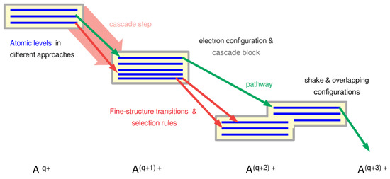
Figure 1.
Important building blocks of all cascade computations. Each cascade is formed by the—list of energetically sorted—levels of electron configurations (blue lines in yellow boxes) from neighbored charge states. These levels are connected to each by fine-structure transitions (red and green arrows, often called lines below) of different kind, and where the number of these transitions rapidly increases with the number of the initial- and final-state levels of the associated configurations. A pathway (green arrows) decribes a possible decay path of an atom and it connects three or more fine-structure levels by different excitation and/or decay processes. Moreover, one or several electron configurations can be comprised together into a single cascade block (gray frames) to properly deal with inter-electronic correlations, but to ensure that each level just belongs to one block. Apart from those configurations of an atomic cascade, which are readily derived from the atomic shell model, further shake configurations can also be considered, although this incorporation typically results in a sizeable increase of the overall complexity. Finally, pairs of cascade blocks give rise to one or several cascade steps (wide light-red arrow) in order to deal with the different atomic processes, and that occur during the relaxation of the atom or ion. The formal decomposition of a cascade into these building blocks suggests various cascade approaches, as explained in the text below.
For one or a few inner-shell holes in an (initial) electron configuration, the release of further Auger electrons quickly leads to complex shell structures with tens (or more) fine-structure levels for each single configuration. This rapid increase of the number of fine-structure levels clarifies the complexity of most cascades, as many, if not all, of these levels might be temporarily populated during the decay of an atoms, and as each level itself may be part of quite many different pathways. Clearly, this complexity must be captured by any realistic cascade model. However, simplifications in the computational treatment may be achieved by the (quantum-mechanical) representation of the levels and by tuning the account of the inter-electronic interactions. Below, we shall introduce and discuss these simplifications in terms of different cascade approaches, and that are further explained in Section 3.3.
2.2. Role of Many-Electron Amplitudes
All of the atomic processes, as mentioned above, have been described in good detail in the literature, and they are usually characterized in terms of their rates or cross sections. Theoretically, these rates are often expressed in terms of many-electron (quantum) transition amplitudes that connect an initial and final fine-structure level, and that are typically even specific to some particular subline (channel), owing to the expansion of the photon field or free-electron waves. Therefore, any successful model of atomic cascades needs straight and quick access to these many-electron amplitudes in order to be able to follow any pathway during the (de-) excitation of the atom or ion, and where the final level of any decay step generally becomes the initial level of the next step. Here, multi-configuration expansions of atomic state functions (ASF), and especially the multi-configuration Dirac–Hartree–Fock method [31], has the advantage that cascades are readily formulated in terms of such many-electron amplitudes (matrix elements), and that they can be applied also to (highly) excited as well as open-shell structures across the periodic table. For cascades and angle- or polarization-resolved studies; indeed, the consequent use of many-electron amplitudes gives rise to compact expressions when compared, for instance, with many-body perturbation or coupled-cluster theory [32].
Indeed, the Jac toolbox [21,22] has been built upon these many-electron amplitudes and it makes use of them in order to compute energy shifts, rates, and cross sections for a large number of processes and for quite different experimental scenarios. These amplitudes generally combine two atomic bound states of the same or two different charge states, and often also include free electrons in the continuum. The use of these amplitudes in Jac also enables us to formulate (and implement) all of the cascade computations in a language that remains close to the formal theory. This is quite in contrast to most other atomic structure codes that are often based on further decompositions of these (many-electron) amplitudes into one- and two-particle (reduced) matrix elements, or often even into radial integrals, well before any implementation or coding is done. The consequent use of these many-electron amplitudes also facilitates the implementation of second- and higher-order processes, once an appropriate (intermediate ASF) basis has been constructed for some given process and help apply them to the time-independent [33,34,35] or even time-dependent density matrix theory [36].
In practice, there are only five types of these many-electron amplitudes that frequently occur in the computation of the electronic structure, properties, and processes of atoms, and that basically refer to different (inner-) atomic interactions. Apart from the electron-electron and electron-photon interaction amplitudes, which are most relevant for all atomic cascades, the (hyperfine) interaction with the nuclear moments [37,38], the mass- and field-shift amplitudes [39,40], or the Coulomb excitation by charged particles [41] are known to determine the behavior of atoms.
2.3. Key Elements for Building Atomic Cascades
Formally, an atomic cascade can be modeled by the set of pathways and all of the quantum amplitudes that pairwise relate the levels in each pathway, and from which the rates and cross sections can be readily derived whenever required. One just needs to follow all of the paths by starting from an initial set of levels. However, in practice, this rather obvious strategy becomes quickly unfeasible due to the large number of pathways and because the many-electron amplitudes are indeed expensive to compute. Therefore, an atomic cascade is better decomposed into (cascade) blocks that comprise all levels of one or several configurations. For each of these blocks, all of the associated levels are then described by a common self-consistent field as well as Hamiltonian matrix, and that accounts for the full configuration mixing within this group of levels. Typically, these blocks are internally constructed from a generated list of configurations as obtained by systematically replacing the shell occupation, and based on quite simple energetic arguments. In a first treatment of a cascade, each contributing configuration hereby often forms an individual cascade block, although several configurations might also be grouped together, in addition, in order to account for relevant—intra or inter-shell—correlations, a feature that has not yet been realized in the present implementation below. In fact, good physical insight is typically required to anticipate the important mixings within the same or different shells, and to make full use of such enlarged configurations blocks.
The blocks of a cascade are then pairwise combined in order to form (so-called) steps of a cascade. For a given process, such as the autoionization or radiative decay of an atom, only steps with at least one non-zero transition amplitude need to considered here, and that can be read-off from just the occupation of the underlying configurations and, perhaps, by using further selection rules. Therefore, different decay processes usually refer to different pairs of configurations, although, in principle, the same pair can be also connected by different steps (atomic processes). For instance, the autoionization [42] and radiative autoionization [43] naturally combine the same blocks of a cascade, but where the (second-order) radiative Auger process is usually well suppressed, analogue to the case for single and multi-photon transitions. In practice, most of the limitations in modeling atomic cascades already arise much earlier and make the discussion of such second-order processes rather obsolete.
Still, the number of cascade blocks and steps does increase quite rapidly with (i) the number of electrons that need to be replaced, (ii) the number of processes that are taken into account into the overall relaxation of the system, and (iii) the depth of the cascade, i.e., the maximum number of electrons that can be released or sought to be considered for a particular cascade. Because these blocks and steps can be readily determined prior to all detailed computations, they also help the user to grasp the “size” of cascade computations and to decide which of these computations are still feasible (and which perhaps not). Furthermore, for each cascade step, the associated (non-zero) many-electron amplitudes are then calculated and kept for later use in order to simulate the desired (line) spectra.
While the distinction of individual blocks and steps of a cascade has been found very useful for all practical purposes, this discrimination obviously fails when the relaxation is affected by (quantum) interferences of different pathways [44,45]. If, for example, the fine-structure splitting of two or more intermediate levels (for two subsequent Auger steps) is small or comparable to the natural line widths of these levels, the angular emission of the emitted Auger electrons can no longer be described by an incoherent summation over individual pathways [46,47]. However, these interferences of quantum amplitudes due to indistinguishable pathways play a minor role for most cascades and are not considered here, as they will require a (much) more elaborate framework.
3. Modeling of Atomic Cascades
3.1. Spectroscopic Observations
While many (spectroscopic) observations are either affected by or directly result from cascade processes, quite different outcomes are recorded by different communities (electrons, photons, coincidences, …) and for different set-ups of the measurements (geometry, resolution, or if even different properties of the emitted particles are to be considered). The large variety of physical scenarios makes it unfeasible, or at least highly impracticable, to implement cascade models for each of these scenarios or set-ups separately. This becomes even more true if, as outlined above, cascades are affected by different radiative and nonradiative processes. Moreover, many of these observations can be readily traced back to the same (single-step) processes and amplitudes and, hence, make a re-calculation of these amplitudes unnecessary, not to say cumbersome.
In order to deal with this situation, we shall further distinguish below between cascade computations and simulations. A cascade computation hereby results into various lists of amplitudes as associated with the selected processes and steps of the cascade. These “line” lists are then the basis for (as well as the computational interface to) all subsequent cascade simulations, and that often need to be analyzed in close contact with experiment. However, by having quite simple access to such lists of transition data (with more or less full physical specification of all the fine-structure levels involved), it is not difficult to add further amplitudes or rates or to deal with other excitation and decay processes.
3.2. Cascade Schemes
Cascade computations are generally performed with the goal to calculate and collect the many-electron amplitudes (and rates) for all steps of the cascade as they are needed in order to simulate the requested spectra. Apart from the relaxation (decay) of the atoms or ions, this must often include the initial excitation due to their interaction with different external fields and particles. Once excited, the atoms then stabilize towards some ionic ground state. Thereby, one or several electrons may be emitted during this relaxation process, if the initially excited level is embedded into the continuum of the next higher charge state (or even beyond). To deal with such different physical scenarios for the excitation and initialization of the cascade, different cascade schemes are distinguished in the implementation below and they are treated by independent computations. Figure 2 displays the most often occuring cascade schemes, and that are further explained in Table 1. These schemes are already (partly) supported in Jac, although other schemes are possible and they might be added in the future. Apart from the frequent photoexcitation or ionization schemes, this includes, for instance, the initial capture of electrons or muons, or their (standard) stepwise decay.
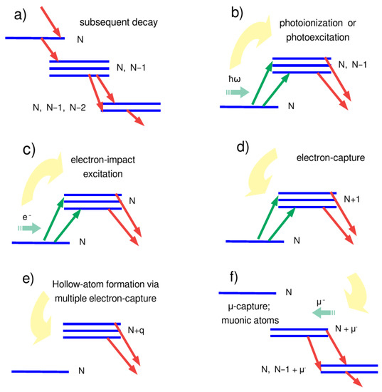
Figure 2.
Simplified view of frequently occuring cascade schemes. Apart from (a) the stepwise decay of an initial N-electron hole-state configuration of an ion via two or more intermediate cascade blocks, including bound levels with less than (the initially) N electrons, these schemes also help account for the excitation of the atoms or ions. Such an excitation may arise from the (b) photoexcitation or photoionization, (c) electron-impact excitation, (d) radiative or dielectronic capture of electrons, (e) the formation of hollow ions via multiple electron capture, or (f) by a muon capture.

Table 1.
Cascade schemes, as (partly) implemented and supported by the Jac toolbox. These schemes help to distinguish cascades of different context and complexity. They internally refer to separate kinds of cascade computations, cf. Section 3.3 and the data structures below.
Overall, a cascade model is often built upon several of such schemes (computations), and that result in various lists of amplitudes (one for each selected atomic process).
3.3. Cascade Approaches
Indeed, atomic cascades may require an enormous computational effort in order to generate, simulate, and interpret all of the data, as needed for modeling a given experiment. Any computation hereby starts from setting up the cascade tree, i.e., the list of configurations, their arrangement into blocks, as well as the selection of all relevant steps of the cascade due to the user-allowed (decay) processes. In most cases, these lists of configurations are automatically generated and (may) serve as starting point in order to group configurations into the cascade blocks. However, the major computational effort refers to the representation of the fine-structure levels for each cascade block as well as to the computation of the transition amplitudes. Several (tens of) thousand or even more of such amplitudes might be required for a mid-size cascade. This is in strong contrast to most atomic structure calculations, which are usually based on just a handful of such many-electron amplitudes. Therefore, it is both necessary and desirable to differentiate between various cascade approaches and to establish a hierarchy of useful approximations. These approaches mainly differ in the generation and use of the orbital functions, the set-up of the Hamiltonian matrix, or the treatment of electronic correlations (configuration mixing) for the representation of the ASF. Furthermore, the hierarchy of these approaches should be designed in such a way to support a systematic improvement of the overall cascade model, while the computations have to be kept feasible for at least the simplest approach in this grouping.
Four such approaches are currently distinguished within the Jac toolbox [21], and that we shall briefly summarize here. They can be controlled by providing a proper set of parameters prior to the computations, and where further details are given in the User Guide & Compendium to Jac [22].
- (i)
- Average single-configuration approach (AverageSCA): this is likely the simplest way to model a cascade in terms of its fine-structure levels and transition amplitudes. Here, the representation of ASF levels is significantly simplified, as they are (all) approximated by single configuration state function (CSF), and they are based on a common set of orbitals, as generated for the initial levels. Indeed, this approach neglectss all configuration mixing between the bound-state levels and, in addition, restricts the computations (by default) to the Coulomb interaction among the electrons, the electric-dipole (E1) transition amplitudes as well as to just a single set of continuum orbitals for each step of the cascade. However, the AverageSCA approach appears to be feasible for (almost) all atoms and ions from the periodic table, although (much) further work is necessary to understand how well this (very) simple approximation is able to describe the underlying relaxation of the system.
- (ii)
- Single-configuration approach (SCA): this approach still uses a common set of orbitals for all electron configurations (cascade blocks) from the same ionization stage, but includes configuration mixing within each block (i.e., by just taking into account the intermediate coupling effects, but not the so-called interaction of configurations). While most other limitations are quite similar to the AverageSCA approach above, the continuum orbitals are generated here for the correct fine-structure (transition) energies, although without the exchange interaction with the bound electrons [48].
- (iii)
- Multiple-configuration approach (UserMCA): this approach facilitates the incorporation of configuration mixings (electron–electron correlations) between user-selected configurations. Apart from some obvious rules for combining inner-shell configurations, the user is encouraged here to explicitly group different configurations together, based on physical insight into the cascade process [49,50]. The arrangement of the bound-state configurations into different groups is usually done either by means of their mean energy, a maximum size (number of CSF) of any individually selected cascade block, or need to be based upon some prior knowledge about strongly interacting configurations. However, care has to be taken by the user to ensure that each physical level (uniquely) belongs to just one group, so that “double counting” of rates, etc., does not occur in the subsequent simulations.
- (iv)
- Multiple-configuration-shake approach (ShakeMCA): this has been designed so far only but will help incorporate also shake-down and shake-up configurations, which do nominally not arise in any standard autoionization schemes of the atom or ion. These shake configurations can then be treated either as individual block of configurations or together with other configurations of the decay cascade. The UserMCA and ShakeMCA approaches will both enable one in the future to incorporate all major electron–electron correlations into the cascade computation by choosing proper “groups” of configurations, while the admixtures from other groups are still neglected.
For this given hierarchy of cascade approaches, the mean computational effort is expected to increase by (at least) one or even several orders of magnitudes in going from one approach to the next more sophisticated one. Therefore, these cascade approaches should be clearly discernible from each other, although it is likely that not all of them will be feasible for the majority of atoms and ions. With this hierarchy, however, the “cost” of any simpler approach will be negligible, when compared to those of the best, but yet feasible cascade model. Moreover, the refinement of this hierarchy is possible by choosing different physical parameters, e.g., by considering more processes, other multipoles, or simply by a better treatment of the continuum for each individual approach.
3.4. Cascade Computations
The computational effort in compiling the cascade tree and all (many-electron) amplitudes suggests, right from the beginning, to separate the cascade computations from the subsequent simulations. Often, several of these cascade computations need to be performed in order to generate all data for the initial excitation of the atoms or ions as well as their subsequent decay. Furthermore, and quite general, each of these computations are split into several independent parts, and that can be summarized, as follows:
- Specification of the cascade tree, which means of all those configurations, whose levels are relevant for the observed spectra. Apart from a simple re-occupation of electron shells, this specification often requires insight by the user into important shake processes, as well as the mixing with other configurations that are energetically nearby.
- The set-up of the cascade blocks and generation of a self-consistent field, or, at least, a proper set of bound-state orbitals. In more detail, this refers to the selection and arrangement of configurations into some many-electron (CSF) basis, in which the atomic states are represented by diagonalizing the associated Hamiltonian matrix.
- The determination of the cascades steps and computation of the associated transition amplitudes and rates. A separate list of such bound-state transitions, i.e., amplitudes and rates, is then compiled for each atomic process of the cascade, such as photoionization, photoemission, autoionization, or others.
- Output of these (line) lists to some interface, either to disc or some Julia dictionary. In practice, all of these lists of transition data are subtypes of a common data structure, from which the desired information can be extracted subsequently.
In a cascade computation, no attempt is made internally to decide that all relevant data are indeed computed or that all of the computed data are relevant for the simulations below. The proper choice and control of these cascade computations require physical perception by the user that goes well beyond of any entirely formalized procedure.
3.5. Cascade Simulations
While the cascade computations just generate all of the the necessary, and often rather expensive (many-electron) transition amplitudes and rates, a cascade simulation makes use of these data in order to derive ion, photon or electron distributions, rate coefficients, or any other information. These cascade simulations are much faster than the prior computations, and often quite similar simulations are repeatedly performed for different initial level occupations, energy ranges, or even different spectra, based on the same data. These simulations need to be guided, or sometimes the code even extended, by the user in order to extract the relevant information. As pointed out before, the user has to make sure that all of the physical-relevant transition data were generated by some prior cascade computation(s), and that they can be uniquely distinguished by the subsequent cascade simulation. Because of the complexity of (most) cascades, special care has to be taken to ensure the consistency of all generated data.
A number of (standard) distributions are frequently required in simulating or modeling atomic cascades. Table 2 shows several of these distributions, as partly implemented and supported by the Jac program. Further simulations will likely be supported as the need arises from the user’s side.
Table 2.
Frequently required distributions in atomic cascade simulations. These distributions are (partly) implemented and supported by the Jac toolbox.
Typically, cascade simulations require to follow (in time) the flux of quantum probability, starting from some initial level population. The detailed re-population of levels in course of the cascade determines the distribution of the emitted electrons and photons, the final charge states, as well as many other observables. Different methods can be applied to propagate the quantum probability through a cascade. In the Jac toolbox, we presently propagate the (occupation) probabilites of the atomic levels until no further changes occur in the level population. Alternative methods refer to the use of rate equations or Monte-Carlo techniques by randomly generating pathways and by utilizing the corresponding transition amplitudes.
4. Implementation of Atomic Cascades
4.1. The Jac Toolbox
Little needs to be said about Jac, the Jena Atomic Calculator, which has been described elsewhere [21], and can readily be downloaded from the web [22]. This toolbox facilitates atomic (structure) calculations of different kind and complexity, and it can be applied without much prior knowledge of the code. For example, the (so-called) Atomic.Computation’s are based on explicitly specified electron configurations and (may) provide level energies, the representation of ASF, or selected level properties. These (atomic) computations also help to evaluate the transition amplitudes (and rates) for all of the processes mentioned above. These features make the Jac toolbox altogether well suited for studying atomic cascades.
For atomic cascades, it is crucial to integrate different atomic processes within a single computational framework in order to ensure good (self-) consistency of the generated data. This then also requires a flexible user interface and simple communication between the different parts of the program. Here, indeed, Jac provides an easy-to-use and powerful platform to extend atomic theory towards the modeling of atomic cascades. It is based on Julia, a new programming language for scientific computing, and that includes a number of (modern) features, such as dynamic types, optional type annotations, type-specializing, just-in-time compilation of code, dynamic code loading, as well as garbage collection [51,52]. Moreover, Julia’s careful design allows the user to gradually approach modern concepts in scientific computing.
4.2. Bulding a Cascade Model
For modeling advanced atomic cascades, we already saw that we need to separate the (physics) scenario, e.g., the set-up and computation of the cascade tree, from the subsequent simulations as well as the display of the requested spectra. Moreover, often, cascade computations have to be done for different schemes to first generate all of the required hole-state configurations or levels, and that then relax by a stepwise decay scheme towards some final ionic levels; cf. Section 3.2. To perform such calculations, Jac provides the data structure Cascade.Computation that enables the user to specify a (cascade) scheme and approach, along with all further input parameters. Figure 3 shows the internal definition of this data structure, while Table 1 displays a number of frequently occuring cascade schemes that are (partly) implemented and supported by the Jac toolbox. All of these schemes are subtypes of an abstract data structure AbstractCascadeScheme and they are used to set the input data that are specific for a given casade computation. Figure 4 displays the explicit internal definition of two of these subtypes (schemes), namely the StepwiseDecayScheme and the PhotonIonizationScheme.
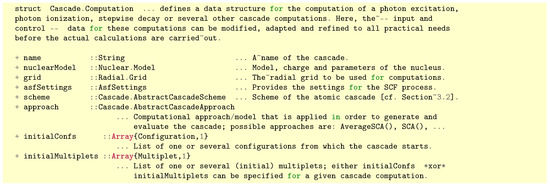
Figure 3.
Definition of the data structure Cascade.Computation in Jac that helps to specify all relevant data about a cascade computation as described in Section 3.4. This structure enables the user to select both, a cascade scheme::Cascade.AbstractCascadeScheme and (cascade) approach::Cascade.AbstractCascadeApproach in order to distinguish different computational models for a cascade.
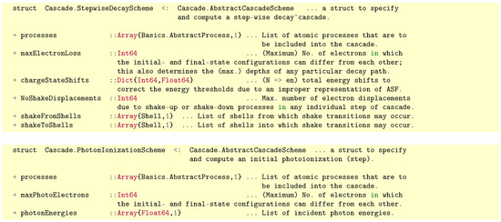
Figure 4.
Definition of the data structures Cascade.StepwiseDecayScheme (upper panel) and Cascade.PhotonIonizationScheme (lower panel) in Jac. For each of these structures, different information must be given to control the corresponding cascade computations. In particular, the subfield processes::Array{Basics.AbstractProcess,1} allow the user to specify the processes, such as Auger(), Radiative(), ..., and which are taken into account to determine the cascade blocks.
Indeed, these and a few other data structures are very central to the implementation of atomic cascades in Jac. A few of them are shown and briefly explained in Table 3, in addition to those already mentioned in Table 1 and Table 2. These data types facilitate the user to map the internal complexity of a given cascade (model) upon the computations to be done. The internal definition of the data structures can be readily obtained at the Julia Repl [53] by typing, for instance,
Table 3.
Selected data structures of the Jac toolbox that are relevant for cascade computations and simulations.

The examples from Figure 4 show how cascade models can be built-up, and specified in detail with all their input data, in order to deal with rather complex scenarios, and which we shall now demonstrate by a simple example below.
4.3. Stepwise Decay of a K-Shell Hole in Atomic Magnesium. An Explicit Example
For the sake of simplicity, here let us restrict to the stepwise autoionization and photon emission of atomic magnesium with an initial K-shell hole. In Jac, a cascade computation for the decay of the configuration is done by scripting:

By this script, we first specify a stepwise decay for the cascade scheme, along with all of the necessary input, as displayed in the upper panel of Figure 4. For this decay, we assume the (single) Auger and photon emission as the dominant processes and consider the emission of up to three electrons from the system (e.g., the depths of the cascade). Of course, the decay of the atoms may stop earlier than this depths, if Auger electrons can no longer be energetically emitted. Moreover, no shake configurations are considered here. In addition, we shall use a logarithmic-linear grid, as appropriate for electron-emission processes as well as a (default) Fermi model with nuclear charge for the nucleus. An average single-configuration (cascade) approach [cf. Section 3.3] is utilized for the representation of all atomic levels involved as well as the calculation of the transition amplitudes, starting from the initial configuration. After having specified this input, all that is finally needed is to perform(..) the computation, and where the optional parameter output=true tells the program that the generated lists of transition data are to be returned as a Julia dictionary (Dict). Any cascade computation returns one (or a few) such list that comprises all lines of the same type, but that may occur here in any order with regard to their transition energies, level specification, or even the charge state of the ions. These “line” lists are the expensive parts of any cascade computation and, hence, are often also stored on a disk; they form the input for all subsequent cascade simulations. In the example above, these final lists are an instance of Cascade.DecayData <:Cascade.AbstractData that comprises the Auger and radiative (lists of) lines.
During the computation, a good deal of information is printed to screen (or, more precisely, to the standard out stream) and, if requested, also to a summary file. Figure 5 displays a minor part of this output that the user should check for the consistency of the input data and computations that are done internally. Apart from the initial levels (multiplet), this standard printout list the (tree of) electron configurations, the generated blocks and steps of the cascade, as well as a summary of all generated continuum orbitals and transition amplitudes. This enables the user to analyze and follow the computations and to understand possible bottlenecks due to the specification and size of the internal steps. Moreover, in the course of these computations, many decisions are made on the basis of default values, which can be overwritten within the code and that may also affect the final results. In particular, the (default) assumptions of the various cascade approaches can be overwritten quite easily, concerning, for instance—the number and type of—the multipoles, a maximum number of partial waves, or how these continuum orbitals are to be generated.
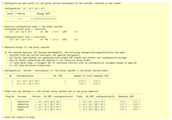
Figure 5.
Selected printout from the example in Section 4.3. Apart from the initial levels (multiplet), this printout lists the cascade tree, the generated blocks, and steps of the cascade, as well as a summary of all generated continuum orbitals and transition amplitudes. This printout can indeed be quite long, but it enables the user to reconstruct the individual calculations and check for inconsistencies or warning that are issued during the execution.
4.4. Running Cascade Simulations
Insight into the set-up of an experiment, its geometry, detectors, as well as into possible limitations of the set-up, is typically required in order to extract the relevant information from a cascade and compare with given measurements. An initial K-shell hole, as in the example above, generally leads to characteristic ion, electron, and photon spectra, and that are affected not only by the initial excitation process, but also the set-up and resolution of the detectors. Cascade simulations aim to utilize the transition amplitudes from the previous computations and combine them in such a manner that accounts for all conditions of some particular experiment or measurement. Obviously, the transition data (amplitudes and rates) from the same cascade computation can hereby give rise very different spectra and distributions.
For an initial K-shell whole in atomic magnesium, a first and simple request may refer to the final ion distribution. Using the results from the last section, given here by the variable data, this distribution of the ionic charge states can be obtained by the following cascade simulations:

With this short script, we just tell Jac that the lowest level of the (initial) hole state configuration is initially populated with probability 1.0, and that we request the ion distribution [cf. Table 2] from these simulations. All of the other steps proceed quite similar as before and eventually provide us with a short table, as displayed above. As seen from this output, our single cascade model predicts that 4.6 % of all ions become eventually doubly ionized, 95.4 % triple ionized, and that any further autoionization is energetically forbidden (within the given model), if we start from the level of -ionized magnesium. The tiny contribution of singly-charged ions (0.02 %) results from the emission, as also taken into account. Quite analogue (cascade) computations and simulations can be performed also for an initially excited configuration , but without showing any of the printout. Figure 6 displays the level structure of these two configurations, together with different ion distributions. Apart from a singly-populated level, as in the example above, here we can also assume a statistical distribution of the levels.
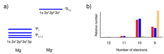
Figure 6.
(a) Level structure of the excited neutral and ionized atomic magnesium. (b) Comparison of the final ion distribution for the hole-state levels as obtained in the averaged single-configuration approach (AverageSCA). Relative ion distribution are shown for an initially occupied level of neutral Mg (red bars), a statistical distribution of all four levels (blue bars) for the ionized level of Mg (orange bars). The small difference between the red and blue bars arises from the contributions of different decay paths.
Of course, the same cascade is also accompanied by a photon (and electron) spectrum that can be simulated similarly by

Accordingly, at least, the basic concept of these simulations in Jac. For these spectra, the user may wish to restrict the photon (electron) energies or to address even more advanced questions concerning the angle distribution or polarization of the emitted photons. However, at present, by far not all of these possible features have yet been realized within the Jac toolbox, but will require further work and requests from the user’s side.
5. Summary and Outlook
To model the excitation and subsequent decay of atoms and ions, we have classified and implemented atomic cascades within the framework of Jac. This classification is based on a clear distinction between cascade computations, to first generate all of the necessary transition data, and subsequent simulations in order to properly combine these data and compare them with experiment. Moreover, for the computations, we also introduced a number of cascade schemes to decompose a given physics scenario into well separated parts, while a hierarchy of (cascade) approaches is applied for keeping the computations feasible overall. These approaches mainly concern the (quantum-mechanical) representation of the level structures and, thus, help to understand the role of atomic interactions and inter-electronic correlations upon the observed spectra. Therefore, our classification of atomic cascades will help provide data for the modeling of astrophysical spectra, similar to Ref. [54], as well as at various places elsewhere [55].
As shown in this work, any implementation of atomic cascades must be based on a rather concise language that combines a proper categorization of different scenarios with a modern code design, a reasonable detailed documentation of the code as well as features for integrated testing. In particular, typical computations and the generated data should be handled rather similarly to how they are used in spoken language or by a pseudo-code. With the Jac toolbox, we provide a computational framework that is flexible enough for further refinements and for more complex shell structures of the atoms and ions, for which the excitation and decay dynamics can be modeled in detail.
While the present implementation has been focused upon (excitation and) decay cascades, especially including inner-shell electrons, there are many other applications that are closely related to atomic cascades. A few examples include the calculation of absorption cross sections, which may be affected by quite different electron–photon interaction processes, or plasma rate coefficients. Both of these applications have been indicated above, but not yet worked out in detail. In the future, we shall use the conceptional and computational basis of Jac in order to enlarge the program towards these demands. However, obviously, this task is much larger that what we can (and plan to) implement. Because Jac is available on Github [22], the code can be readily forked and extensions reported in order to deal with more complex cascades.
Author Contributions
Methodology, S.F., P.P., S.S.; software, S.F.; writing—review and editing, S.F., P.P., S.S. All authors have read and agreed to the published version of the manuscript.
Funding
This research was funded in part by the German Federal Ministry for Education and Research (BMBF) within the “Verbundforschung” funding scheme under contracts 05K19RG3 and 05K16SJA.
Institutional Review Board Statement
Not applicable.
Informed Consent Statement
Not applicable.
Data Availability Statement
Not applicable.
Conflicts of Interest
The authors declare no conflict of interest.
References and Note
- Mirakhmedov, M.N.; Parilis, E.S. Auger and X-ray cascades following inner-shell ionisation. J. Phys. 1988, B21, 795. [Google Scholar] [CrossRef]
- Kucas, S.; Drabuzinskis, P.; Kynienė, A.; Masys, S.; Jonauskas, V. Evolution of radiative and Auger cascades following 2s vacancy creation in Fe2+. J. Phys. B 2019, 52, 225001. [Google Scholar] [CrossRef]
- Schippers, S.; Borovik, A.; Buhr, T.; Hellhund, K.; Holste, K.; Kilcoyne, A.L.D.; Klumpp, S.; Martins, M.; Müller, A.; Ricz, S.; et al. Stepwise contraction of the nf Rydberg shells in the 3d photoionization of multiply-charged xenon ions. J. Phys. B 2015, 48, 144003. [Google Scholar] [CrossRef]
- Schippers, S.; Beerwerth, R.; Abrok, L.; Bari, S.; Buhr, T.; Martins, M.; Ricz, S.; Viefhaus, J.; Fritzsche, S.; Müller, A.; et al. Prominent role of multi-electron processes in K-shell double and triple photodetachment of oxygen anions. Phys. Rev. A 2016, 94, 041401. [Google Scholar] [CrossRef]
- Khalal, M.A.; Lablanquie, P.; Andric, L.; Palaudoux, J.; Penent, F.; Bučar, K.; Žitnik, M.; Püttner, R.; Jänkälä, K.; Cubaynes, D.; et al. 4d-inner-shell ionization of Xe+ ions and subsequent Auger decay. Phys. Rev. A 2017, 96, 013412. [Google Scholar] [CrossRef]
- Ma, X.; Stöhlker, T.; Bosch, F.; Brinzanescu, O.; Fritzsche, S.; Kozhuharov, C.; Ludziejewski, T.; Mokler, P.H.; Stachura, Z.; Warczak, A.; et al. State–selective electron capture in He–like U90+ ions colliding with gaseous targets. Phys. Rev. A 2001, 64, 012704. [Google Scholar] [CrossRef]
- Ueda, K.; Shimizu, Y.; Chiba, H.; Kitajima, M.; Tanaka, H.; Fritzsche, S.; Kabachnik, N.M. Experimental and theoretical study of the Auger cascade following the 2p→4s photoexcitation in Ar. J. Phys. B 2001, 34, 107. [Google Scholar] [CrossRef]
- Kabachnik, N.M.; Fritzsche, S.; Grum-Grzhimailo, A.N.; Meyer, M.; Ueda, K. Coherence and correlations in photoinduced Auger and fluorescence cascades in atoms. Phys. Rep. 2007, 451, 155. [Google Scholar] [CrossRef]
- Le Bigot, E.O.; Boucard, S.; Covita, D.S.; Gotta, D.; Gruber, A.; Hirtl, A.; Fuhrmann, H.; Indelicato, P.; dos Santos, J.M.F.; Schlesser, S.; et al. High-precision X-ray spectroscopy in few-electron ions. Phys. Scr. 2009, T134, 014015. [Google Scholar] [CrossRef]
- Gillaspy, J.D. Precision spectroscopy of trapped highly charged heavy elements: Pushing the limits of theory and experiment. Phys. Scr. 2014, 98, 1114004. [Google Scholar] [CrossRef]
- Andersson, J.; Beerwerth, R.; Linusson, P.; Eland, J.H.D.; Zhaunerchyk, V.; Fritzsche, S.; Feifel, R. Triple ionization of atomic Cd involving 4p−1 and 4s−1 inner-shell holes. Phys. Rev. A 2015, 92, 023414. [Google Scholar] [CrossRef]
- Wiese, W.L. Spectroscopic diagnostics of low temperature plasmas: Techniques and required data. Spectrochim. Acta B 1991, 46, 831–841. [Google Scholar] [CrossRef]
- Saha, B.; Fritzsche, S. Influence of dense plasma on the low-lying transitions in Be-like ions: Relativistic multiconfiguration Dirac–Fock calculation. J. Phys. B 2007, 40, 259–270. [Google Scholar] [CrossRef]
- Feldman, U.; Mandelbaum, P.; Seely, J.F.; Doschek, G.A.; Gursky, H. The potential for plasma diagnostics from stellar extreme-ultraviolet observations. Astrophy. J. Suppl. 1992, 81, 387–408. [Google Scholar] [CrossRef]
- Dong, C.Z.; Fritzsche, S.; Fricke, B.; Sepp, W.-D. Branching ratios and lifetimes of the low–lying levels of Fe xx. Mon. Not. R. Astron. Soc. 1999, 307, 809–814. [Google Scholar] [CrossRef]
- Battistini, C.; Bensby, T. The origin and evolution of r- and s-process elements in the Milky Way stellar disk. Astron. Astrophys. 2016, 586, A49. [Google Scholar] [CrossRef]
- Popping, G.; Somerville, R.S.; Trager, S.C. Evolution of the atomic and molecular gas content of galaxies. Mon. Not. R. Astron. Soc. 2014, 442, 2398–2418. [Google Scholar] [CrossRef]
- Jakas, M.M. Many-body effects in atomic-collision cascades. Phys. Rev. Lett. 1985, 55, 1782. [Google Scholar] [CrossRef] [PubMed]
- Schippers, S.; Martins, M.; Beerwerth, R.; Bari, S.; Holste, K.; Schubert, K.; Viefhaus, J.; Savin, D.W.; Fritzsche, S.; Müller, A. Near L-edge single and multiple photoionization of singly charged iron ions. Astrophys. J. 2017, 849, 5. [Google Scholar] [CrossRef]
- Beerwerth, R.; Buhr, T.; Perry-Sassmannshausen, A.; Stock, S.O.; Bari, S.; Holste, K.; Kilcoyne, A.L.D.; Reinwardt, S.; Ricz, S.; Savin, D.W.; et al. Near L-edge single and multiple photoionization of triply charged iron ions. Astrophys. J. 2019, 887, 189. [Google Scholar] [CrossRef]
- Fritzsche, S. A fresh computational approach to atomic structures, processes and cascades. Comput. Phys. Commun. 2019, 240, 1–14. [Google Scholar] [CrossRef]
- Fritzsche, S. JAC: User Guide, Compendium & Theoretical Background. Available online: https://github.com/OpenJAC/JAC.jl (accessed on 10 February 2021).
- Fritzsche, S. Ratip—A toolbox for studying the properties of open—Shell atoms and ions. J. Electr. Spec. Rel. Phenon. 2001, 114–116, 1155–1164. [Google Scholar] [CrossRef]
- Fritzsche, S. The Ratip program for relativistic calculations of atomic transition, ionization and recombination properties. Comput. Phys. Commun. 2012, 183, 1525–1559. [Google Scholar] [CrossRef]
- Barnes, J.; Kasen, D. Effect of a high opacity on the light curves of radioactively powered transients from compact object mergers. Astrophys. J. 2013, 775, 18. [Google Scholar] [CrossRef]
- Kravtsov, A.V.; Borgani, S. Formation of Galaxy Clusters. Annu. Rev. Astrononmy Astrophys. 2012, 50, 353–409. [Google Scholar] [CrossRef]
- Cowan, R.D. The Theory of Atomic Structure and Spectra; University of California Press: Berkeley, CA, USA, 1981. [Google Scholar]
- Fritzsche, S. Large-scale accurate structure calculations for open-shell atoms. Phys. Scr. 2002, T100, 37. [Google Scholar] [CrossRef]
- Perry-Sassmannshausen, A.; Buhr, T.; Borovik, A., Jr.; Martins, M.; Reinwardt, S.; Ricz, S.; Stock, S.O.; Trinter, F.; Müller, A.; Fritzsche, S.; et al. Multiple photodetachment of carbon anions via single and double core-hole creation. Phys. Rev. Lett. 2020, 124, 083203. [Google Scholar] [CrossRef] [PubMed]
- Andersson, J.; Beerwerth, R.; Roos, A.H.; Squibb, J.J.; Singh, R.; Zagorodskikh, S.; Talaee, O.; Koulentianos, D.; Eland, J.H.D.; Fritzsche, S.; et al. Auger decay of 4d inner-shell holes in atomic Hg leading to triple ionization. Phys. Rev. A 2017, 96, 012505. [Google Scholar] [CrossRef]
- Grant, I.P. Relativistic Quantum Theory of Atoms and Molecules: Theory and Computation; Springer: Berlin/Heidelberg, Germany, 2007. [Google Scholar]
- Eliav, E.; Fritzsche, S.; Kaldor, U. Electronic structure theory of the superheavy elements. Nucl. Phys. A 2015, 944, 518–550. [Google Scholar] [CrossRef]
- Surzhykov, A.; Fritzsche, S.; Stöhlker, T.; Tachenov, S. Polarization studies on the radiative recombination of highly charged bare ions. Phys. Rev. A 2003, 68, 022710. [Google Scholar] [CrossRef]
- Surzhykov, A.; Indelicato, P.; Santos, J.P.; Amaro, P.; Fritzsche, S. Two-photon absorption of few-electron heavy ions. Phys. Rev. A 2011, 84, 022511. [Google Scholar] [CrossRef]
- Fritzsche, S.; Grum-Grzhimailo, A.N.; Gryzlova, E.V.; Kabachnik, N.M. Angular distributions and angular correlations in sequential two-photon double ionization of atoms. J. Phys. B 2008, 41, 165601. [Google Scholar] [CrossRef]
- Li, Y.; Ullrich, C.A. Time-dependent transition density matrix. Chem. Phys. 2011, 391, 157–163. [Google Scholar] [CrossRef]
- Charlwood, F.C.; Billowes, J.; Campbell, P.; Cheal, B.; Eronen, T.; Forest, D.H.; Fritzsche, S.; Honma, M.; Jokinen, A.; Moore, I.D.; et al. Ground state properties of manganese isotopes across the N=28 shell closure. Phys. Lett. B 2010, 690, 346–351. [Google Scholar] [CrossRef]
- Yordanov, D.T.; Balabanski, D.L.; Bieroń, J.; Bissell, M.L.; Blaum, K.; Budinčević, I.; Fritzsche, S.; Frömmgen, N.; Georgiev, G.; Geppert, C.; et al. Spins, Electromagnetic moments and isomers of 107-129Cd. Phys. Rev. Lett. 2013, 110, 192501. [Google Scholar] [CrossRef]
- Cheal, B.; Cocolios, T.E.; Fritzsche, S. Laser spectroscopy of radioactive isotopes: Role and limitations of accurate isotope-shift calculations. Phys. Rev. A 2012, 86, 042501. [Google Scholar] [CrossRef]
- Ferrer, R.; Barzakh, A.; Bastin, B.; Beerwerth, R.; Block, M.; Creemers, P.; Grawe, H.; de Groote, R.; Delahaye, P.; Flechard, X.; et al. Towards high-resolution laser ionization spectroscopy of the heaviest elements in supersonic gas jet expansion. Nat. Commun. 2017, 8, 14520. [Google Scholar] [CrossRef]
- Surzhykov, A.; Jentschura, U.D.; Stöhlker, T.; Gumberidze, A.; Fritzsche, S. Alignment of heavy few-electron ions following excitation by relativistic Coulomb collisions. Phys. Rev. 2008, A77, 042722. [Google Scholar] [CrossRef]
- Åberg, T.; Howat, G. Theory of the Auger Effect. In Corpuscles and Radiation in Matter I; Encyclopedia of Physics Vol. XXXI; Mehlhorn, W., Ed.; Springer: Berlin/Heidelberg, Germany, 1982; p. 469. [Google Scholar]
- Verma, H.R. A study of radiative Auger emission, satellites and hypersatellites in photon-induced K x-ray spectra of some elements in the range 20≤Z≤32. J. Phys. B 2000, 33, 3407. [Google Scholar] [CrossRef]
- Brieger, M.; Schuessler, H.A. What is quantum interference in atoms? Eur. Lett. 1996, 35, 1. [Google Scholar] [CrossRef]
- Fritzsche, S.; Nikkinen, J.; Huttula, S.-M.; Aksela, H.; Huttula, M.; Aksela, S. Interferences in the 3p4nl satellite emission following the excitation of argon across the 2p1/254s and 2p3/253dJ=1 resonances. Phys. Rev. A 2007, 75, 012501. [Google Scholar] [CrossRef]
- Shimizu, Y.; Yoshida, H.; Okada, K.; Muramatsu, Y.; Saito, N.; Okashi, H.; Tamenori, Y.; Fritzsche, S.; Kabachnik, N.M.; Tanaka, H.; et al. High resolution angle-resolved measurements of Auger emission from the photo-excited 1s−13p state of Ne. J. Phys. B At. Mol. Opt. Phys. 2000, 33, L685. [Google Scholar] [CrossRef]
- Kitajima, M.; Okamoto, M.; Shimizu, Y.; Chiba, H.; Fritzsche, S.; Kabachnik, N.M.; Sazhina, I.P.; Koike, F.; Hayaishi, T.; Tanaka, H.; et al. Experimental and theoretical study of the Auger cascade following 3d→5p photoexcitation in krypton. J. Phys. B 2001, 34, 3829. [Google Scholar] [CrossRef]
- Fritzsche, S.; Fricke, B.; Sepp, W.-D. Reduced L1 level-width and Coster-Kronig yields by relaxation and continuum interactions in atomic zinc. Phys. Rev. A 1992, 45, 1465. [Google Scholar] [CrossRef] [PubMed]
- Dong, C.Z.; Fritzsche, S. Relativistic, relaxation and correlation effects in spectra of Cu II. Phys. Rev. A 2005, 72, 012507. [Google Scholar] [CrossRef]
- Fritzsche, S.; Froese Fischer, C.; Fricke, B. Calculated level energies, transition probabilities and lifetimes for phosphorus-like ions of the iron group in the 3s3p4 and 3s23p23d configurations. At. Data Nucl. Data Tables 1998, 68, 149–179. [Google Scholar] [CrossRef][Green Version]
- Available online: https://docs.julialang.org/ (accessed on 10 February 2021).
- Bezanson, J.; Chen, J.; Chung, B.; Karpinski, S.; Shah, V.B.; Vitek, J.; Zoubritzky, J. Julia: Dynamism and performance reconciled by design. Proc. ACM Program. Lang. 2018, 2, 120. [Google Scholar] [CrossRef]
- Julia Comes with a Full-Featured Interactive and Command-Line REPL (Read-Eval-Print Loop) that is built into the Executable of the Language.
- Schippers, S.; Beerwerth, R.; Bari, S.; Buhr, T.; Holste, K.; Kilcoyne, A.D.; Perry-Sassmannshausen, A.; Phaneuf, R.A.; Reinwardt, S.; Savin, D.W.; et al. Near L-edge single and multiple photoionization of doubly charged iron ions. Astrophys. J. 2021, 908, 52. [Google Scholar] [CrossRef]
- Sharma, L.; Surzhykov, A.; Srivastava, R.; Fritzsche, S. Electron-impact excitation of singly charged metal ions. Phys. Rev. A 2011, 83, 062701. [Google Scholar] [CrossRef]


Publisher’s Note: MDPI stays neutral with regard to jurisdictional claims in published maps and institutional affiliations. |
© 2021 by the authors. Licensee MDPI, Basel, Switzerland. This article is an open access article distributed under the terms and conditions of the Creative Commons Attribution (CC BY) license (http://creativecommons.org/licenses/by/4.0/).