The Topological Origin of Quantum Randomness

Abstract

What is the origin of quantum randomness? Why does the deterministic, unitary time development in Hilbert space (the ‘$4\pi$-realm’) lead to a probabilistic behaviour of observables in space-time (the ‘$2\pi$-realm’)? We propose a simple topological model for quantum randomness. Following Kauffmann, we elaborate the mathematical structures that follow from a $distinction$ $(A,B)$ using group theory and topology. Crucially, the 2:1-mapping from $SL(2,\mathbb{C})$ to the Lorentz group $SO(3,1)$ turns out to be responsible for the stochastic nature of observables in quantum physics, as this 2:1-mapping breaks down during interactions. Entanglement leads to a change of topology, such that a distinction between A and B becomes impossible. In this sense, entanglement is the counterpart of a distinction $(A,B)$. While the mathematical formalism involved in our argument based on virtual Dehn twists and torus splitting is non-trivial, the resulting haptic model is so simple that we think it might be suitable for undergraduate courses and maybe even for High school classes.

1. Introduction

The stochastic nature of quantum physics is an experimental fact beyond any doubt. The debate on the interpretation and the $origin$ of quantum randomness is as old as quantum physics itself. Max Born brings the core issue of the debate to the point when he asks: “But can our desire of understanding, our wish to explain things, be satisfied by a theory which is frankly and shamelessly statistical and indeterministic?” [1]. One of his famous contemporaries, Albert Einstein, was certainly not satisfied by such kind of theory. He expressed his discontent in a letter to Born, stating famously that he was convinced that “God does not roll the dice.” [2].

Even though most modern physicists disagree with Einstein in this point and accept randomness as a fundamental part of physical reality, many questions on how to interpret the fact that quantum physics is a probabilistic theory are still topic of philosophical dispute. Of central importance in that context is the fact that measurable properties of a quantum system, which are considered part of our accessible physical reality, seem to be inherently random in nature, while their mathematical representations are at all times well-defined. The recognition of this gap between well-defined mathematical representation and observable reality gives rise to several questions, which are closely related to each other.

First of all, it can be asked how both sides of the medal are connected to each other, that is, how randomness comes into play when turning from abstract mathematical formalism to sensually accessible reality. Two well-known and controversial proposals how to conceptualise this transition are the assumption of an instantaneous ‘collapse’ of the wave-function and the ‘many-worlds’ hypothesis. In the present contribution, we propose a topological model for describing the origin of quantum randomness.

Secondly, it can be asked whether and how randomness relates to properties of the quantum system itself. It is helpful to distinguish $epistemic$ and $ontic$ descriptions of quantum systems in this context—while an epistemic description of a quantum system encodes information about the system that is at least in principle empirically accessible, an ontic description of quantum systems refers to an observation-independent reality, regardless if it is empirically accessible or not [3]. Consequently, randomness might emerge from an ontic description of quantum phenomena, hence reflecting some inherent property of quantum objects, or from an epistemic description, meaning that it can somehow be retraced to incomplete knowledge of the system’s properties. In our topological model, which we consider as an ontic description, we see that randomness only emerges due to the fact that not all topological changes are observable in space time, leading to an interpretation of quantum randomness that can be classified as epistemic.

In Section 2, we first want to introduce the haptic model without any reference to its mathematical background and explicit physical interpretation. From a didactical point of view, the haptic model shown in Figure 1 is so simple and intuitive that we think it could be useful in undergraduate lectures, maybe even in High school classes. In the following sections, we derive the mathematical theory which justifies and generalizes our simple model.

In Section 3, following Kauffmann [4], starting with elementary properties of a distinction $(A,B)$, we find quaternions (equivalently, the Pauli matrices) as basic ingredients for the representation of any physical quantity, and in turn, knot theory.

In Section 4, we review our simple haptic model for the 2:1-double cover of $SL(2,\mathbb{C})$ and the Lorentz group $SO(3,1)$ which has already be introduced in [5].

In Section 5, we show that particle representations which follow naturally from the isomorphism between $SL(2,\mathbb{C})$ and $SU\left(2\right)\times SU\left(2\right)$ can be modeled by $Dehn$ $twists$ within our haptic model, providing a link between this well established theory and our haptic model. Geometrically, the group $SU\left(2\right)$ in fundamental representation is just the hypersphere $S_3$. Crucially, we have to distinguish the $4\pi$-realm (with $S_3$ as prototypical example) and the $2\pi$-realm (like $S_2$), with the Hopf-mapping $S_3\to S_2$ being the simplest and most important example for a mapping between both ‘realms’. Our knot theoretic model provides a simple way to illustrate this mapping, as shown later on.

In Section 6, we show that the knot theoretic approach naturally leads to the equations of motion for free particles. Explicitly, we discuss the simplest and most important examples: spin $j=1/2$ and $j=1$. We briefly review gauge interactions, as the transition between topologically equivalent configurations is nothing but a knot theoretic interpretation of gauge freedom. While this work is inspired by previous work from Kauffmann, ref. [4], here we extend this approach and provide a geometric interpretation within our haptic model.

In Section 7, we introduce the counterpart to distinctions, that is, entanglement: Our model suggests that entanglement is increased when decreasing the number of possible distinctions. Crucially, we introduce $virtual$ Dehn twists as a new concept for modeling entanglement as counterpart of distinctions. It seems that our topological approach is consistent with existing theories, in particular, for W and GHZ states (three qubits), HS-states (four qubits) and Dicke states (N qubits). We compare our model with a knot theoretic ansatz advocated by Kauffmann [6] and find that is consistent with our approach.

In Section 8, we extend our model from quaternions to octonions and present a new model for color confinement using virtual Dehn twists with rotation angle $\pi /3$. We also discuss its relation to normed division algebras, and recent approaches to model elementary particles by Furey [7] and Gresgnit [8].

In Section 9, we discuss the relation between distinctions, entanglement, and interactions based on (virtual) Dehn twists and torus splitting. While the distinction leads to the group structure $SU\left(2\right)\times SU\left(2\right)$, in order to $undo$ a distinction, we have to introduce interactions. While the unitary (time) development of quantum states in the $4\pi$-realm is continuous, discontinuities and randomness seem to exist only in the $2\pi$-realm due to the 2:1-mapping, as will be shown with three non-trivial examples. In particular, the simple and intuitive haptic model for quantum randomness as shown in Figure 1, seems to have its deeper origin in the fact that this 2:1-mapping from quantum states into space-time is impossible during interactions, that is, while the topology of the quantum states is changed. We conjecture that only those quantum states are observable which can be reached by virtual Dehn twists and torus splitting.

Finally, in Section 10, we discuss conclusions and possible further applications of our haptic model. Since our ansatz leads to the prediction of a smallest time scale (the Planck time), further applications of the haptic model in relation to quantum gravity seem to be of interest. While a simple distinction $(A,B)$ leads to flat space-time, is is not sufficient to derive curved space-time. This is a clear limitation of the present ansatz and corresponding modeling. We leave it to future work to elaborate further on this point.

While there are many complex and interesting questions waiting for future research, we advocate the striking $simplicity$ of the haptic model for quantum randomness as proposed in Figure 1, which might be of merit also for didactical approaches to quantum and to particle physics.

2. A Simple Haptic Model for Quantum Randomness

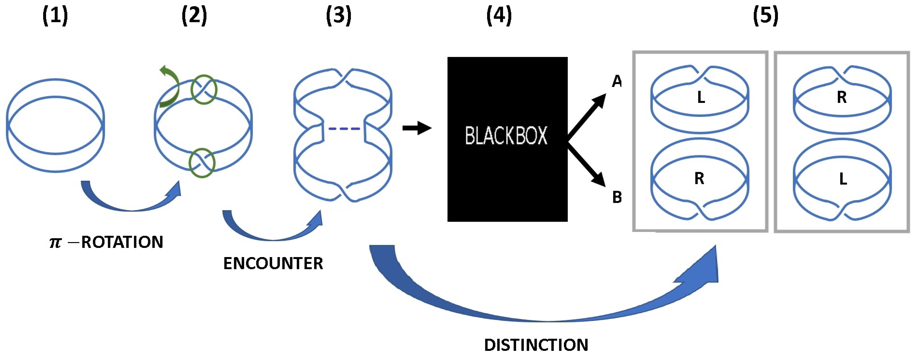
Before making mathematical details explicit, let us first introduce our haptic model as shown in Figure 1: Consider a closed loop (1) and turn it once upside-down (2). As a result, two opposite twists $R,L$ are created, while the global topology of the loop remains unchanged. Next, let two pieces of the loop come close in an encounter (3), where one part of the loop contains the R-twist, the other part the L-twist. Still, the global topology is not changed. Suppose that this configuration is then placed inside a black box (4). Alice and Bob are asked to take one of the two parts of the loop, that is, to separate the two pieces at the position of the encounter.

As a result, the topology of the loop $is$ changed. We obtain two parts A and B, which obviously have the property that one loop has a left twist (L), while the other has a right twist (R). It is not clear whether A receives the right twist, or B (5). Up to this point, we can view this just as a kind of game which can be played even with children. In this game, there is no doubt that the assignment of A and B to the left- and right twist is arbitrary, simply because before doing so, there is no left or right twist—there is only one piece of paper without any twists. The randomness in the assignment of R and L to A and B emerges due to the fact that we have to change the topology in order to $distinguish$ A from B. As we will show in what follows, this is the origin of quantum randomness in our model. In order to see this, we will develop the mathematical formalism of quantum theory starting from the choice to make $distinctions$. Superpositions and entanglement turn out to be the counterpart of a distinction $(A,B)$, leading to interaction and entanglement between A and B, culminating in topological changes such that A and B merge to a single quantum state.

While the paper strip model is the simplest representation for the relation between $distinctions$ and $entanglement$, a more elaborated version of the model has to deal with generalized Dehn twists on a torus, or even Dehn surgery. The key features of our argument, however, remain the same.

3. On the Relation between Distinctions and Space-Time

Following Kauffmann [6], we denote a distinction as $(A,B)$. The only assumption we need is that A, in general, might be different from B in any way. Once we start to make distinctions, we can operate on them in some very obvious manner: Let $\mathrm{id}$ be the identity operations, then a global reflection is defined as

$$\begin{array}{c}\hfill -\mathrm{id}(A,B)\equiv (-A,-B).\end{array}$$

(1)

Distinct objects can be exchanged, which we denote by the operation

$$\begin{array}{c}\hfill \varphi (A,B)\equiv (B,A).\end{array}$$

(2)

Another very obvious operation is a partial reflection, that is, mapping A to $-A$, or B to $-B$,

$$\begin{array}{c}\hfill p(A,B)\equiv (-A,B)\\ \hfill q(A,B)\equiv (A,-B).\end{array}$$

(3)

Of course, operations can be combined, which leads to the interesting property

$$\begin{array}{c}\hfill {\left(\varphi q\right)}^2(A,B)=(-A,-B)=(-1)(A,B).\end{array}$$

(4)

It follows ${\left(\varphi q\right)}^2=-1$. Therefore, the combination $\varphi q$ can be seen as representation of the complex number i. We may write these operations using $2\times 2$ matrices as follows,

$$\begin{array}{c}\hfill \pm \mathrm{id}\simeq \pm \left[\begin{array}{cc}1& 0\\ 0& 1\end{array}\right],\varphi \simeq \left[\begin{array}{cc}0& 1\\ 1& 0\end{array}\right],\mathrm{q}\simeq \left[\begin{array}{cc}1& 0\\ 0& -1\end{array}\right],\varphi q\simeq \left[\begin{array}{cc}0& -1\\ 1& 0\end{array}\right].\end{array}$$

(5)

These four operations are equivalent to the Pauli matrices and the identity operation,

$$\begin{array}{c}\hfill \varphi \simeq {\sigma }_1,\varphi q\simeq -i{\sigma }_2,q\simeq {\sigma }_3,\pm id.\end{array}$$

(6)

It is a matter of convention whether we represent i as $2\times 2$ matrix (in this case, the Pauli-matrices would be $4\times 4$ matrices), or to define a new symbol i with $i^2=-1$. In what follows, we will stick to the latter convention, corresponding to the usual notation.

Using these basic building blocks, we may introduce coordinates in various interpretations. The most straightforward would be real coordinates, that is, space-time itself, which naturally comes with a hermitian structure

$$\begin{array}{c}\hfill h\equiv \mathrm{id}t+\overrightarrow{\sigma }\overrightarrow{r}=\left[\begin{array}{cc}t+z& x-iy\\ x+iy& t-z\end{array}\right],\det h=t^2-{\overrightarrow{r}}^2\end{array}$$

(7)

and the Lorentz group $O(3,1)$ as transformation group leaving $\det h$ invariant. Note that a $distinction$ naturally leads to the four operations as defined in Equation (5), and in turn to four dimensional space-time. If the time coordinate t is replaced by $it$, we obtain the imaginary time-formalism. We adopt the situation of $d=3$ spatial dimensions, and one real time dimension.

4. The $\mathbf{4}\mathit{\pi }$-Realm and the $\mathbf{2}\mathit{\pi }$-Realm: $\mathit{SL}(\mathbf{2},\mathbb{C})$ as Double Cover of the Lorentz Group $\mathit{SO}(\mathbf{3},\mathbf{1})$

Next, using the Pauli matrices with $complex$ coordinates $\{w_1,w_2,w_2\}$, we can define a six dimensional (tangent) space spanned by

$$\begin{array}{c}\hfill u\equiv \overrightarrow{\sigma }\overrightarrow{w},\mathrm{tr}u=0,\end{array}$$

(8)

which is the Lie algebra of the special linear group $SL(2,\mathbb{C})$. The fact that the Pauli matrices are the fundamental building blocks of space-time is reflected in the transformation law

$$\begin{array}{c}\hfill h^{\prime }=e^{+u}h{e}^{-u},\det h^{\prime }=\det h,\end{array}$$

(9)

which indeed is a Lorentz transformation, since $\det h^{\prime }=\det h$. While the existence of an upper limit for velocities follows from the very nature of Lorentz-transformations, it is impossible to find the value of the speed of light c just from a distinction (as is the case for all other fundamental constants of nature). We set $c=1$ in what follows.

Now, we derive explicitly the relation between $SL(2,\mathbb{C})$ and $SO(3,1)$ and propose a simple model for the double cover. We denote by ${\Lambda }_{\mu }^{\nu }\in O(3,1)$ a Lorentz-transformation, defined as the invariance group for the transformation from reference system $x_{\mu }^{\prime }=(t^{\prime },{\overrightarrow{x}}^{\prime })$ to $x_{\nu }=(t,\overrightarrow{x})$, with the metric tensor $\mathrm{diag}{g}_{\mu \nu }=(+1,-1,-1,-1)$. In matrix form, we find ${\Lambda }^{T}g\Lambda =g$. It is well known that $O(3,1)$ can be decomposed into four simply connected parts. Let $O{(3,1)}^{\mathrm{id}}$ be the part of the group connected to the identity operation. Then, we can decompose

$$\begin{array}{c}\hfill O(3,1)=O{(3,1)}^{\mathrm{id}}⨁O{(3,1)}^{\mathrm{id}}\mathbf{P}⨁O{(3,1)}^{\mathrm{id}}\mathbf{T}⨁O{(3,1)}^{\mathrm{id}}\mathbf{PT},\end{array}$$

(10)

where $\mathbf{P}$ is the parity operation $\overrightarrow{r}\to -\overrightarrow{r}$, and $\mathbf{T}$ the time-reversal operation $t\to -t$. Note, that $deth=t^2-{\overrightarrow{r}}^2$ in (7) remains invariant in all four sectors of $SO(3,1)$. The 2:1 mapping with $SL(2,\mathbb{C})$

$$\begin{array}{c}\hfill O{(3,1)}^{\mathrm{id}}\simeq \frac{SL(2,\mathbb{C})}{\{-1,+1\}}\end{array}$$

(11)

is then explicitly given by

$$\begin{array}{c}\hfill {\Lambda }_{\nu }^{\mu }{\sigma }^{\nu }=h{\sigma }^{\mu }{h}^{†},\end{array}$$

(12)

where we introduce the four matrices ${\sigma }^{\mu }$ which define the four operations on a distinction (5),

$$\begin{array}{c}\hfill {\sigma }^{\mu }\equiv (\mathrm{id},{\sigma }_1,{\sigma }_2,{\sigma }_3).\end{array}$$

(13)

Taking the trace, we find

$$\begin{array}{c}\hfill {\Lambda }_{\rho }^{\mu }=\frac{1}{2}\mathrm{tr}\left(h{\sigma }^{\mu }{h}^{†}{\sigma }_{\rho }\right)\end{array}$$

(14)

with $h\in SL(2,\mathbb{C})$.

What is of importance for our reasoning is the fact that $SL(2,\mathbb{C})$ is the two-fold covering group of $SO{(3,1)}^{\mathrm{id}}$, meaning that $4\pi$-rotations in $SL(2,\mathbb{C})$ are mapped to two traversals of $2\pi$-rotations in $SO(3,1)$. Note that this 2:1-mapping only emerges for four-dimensional space-time, since $\dim SO(d,1)=d(d+1)/2$ matches $\dim SL(n,C)=2n^2-2$ only for the single combination $\{d=3,n=2\}$. Recently, we introduced a simple paper strip model for a haptic encoding of this double cover by re-gluing the pieces $(0,2\pi )$ and $(2\pi ,4\pi )$. Since this regluing can be done in two different manners, in general, we have to think of a torus in $SO(3,1)$, as shown in Figure 2.

The true power of this simple model becomes visible once we introduce (Dehn) $twists$ in combination with the 2:1 mapping in order to represent free particles [5,9].

5. How Particles in Space-Time Emerge from Making Distinctions

The six dimensional Lie algebra of $SL(2,\mathbb{C})$ defined in (8) generates boosts and rotations on space-time as given by Equation (9). However, rotations and boosts do not commute. Let $J_i$ be the three generators of rotation, and $K_i$ be the three generators of boosts, then we find the commutators

$$\begin{array}{c}\hfill [J_i,J_j]=i{\epsilon }_{ijk}{J}_k,[J_i,K_j]=i{\epsilon }_{ijk}{K}_k,[K_i,K_j]=-i{\epsilon }_{ijk}{J}_k.\end{array}$$

(15)

We can decompose this algebra into two independent $SU\left(2\right)$-algebras by defining

$$\begin{array}{c}\hfill A\equiv \frac{1}{2}(J+iK),B\equiv \frac{1}{2}(J-iK),\end{array}$$

(16)

and we find

$$\begin{array}{c}\hfill [A_i,A_j]=i{\epsilon }_{ijk}{A}_k,[B_i,B_j]=i{\epsilon }_{ijk}{B}_k,[A_i,B_j]=0.\end{array}$$

(17)

Thus, both sets of operators $A_i,B_j$ generate two independent angular momentum algebras. Each angular momentum algebra allows for a set of representations with spin $\{0,1/2,1,\dots \}$. Let $\{a,b\}$ denote the spins in representation A and B. Then, each of the representations have dimension $(2a+1)$ and $(2b+1)$, respectively.

It is fascinating to see that according to the decomposition (16), the combination of two $SU\left(2\right)$-algebras is intimately related to space-time transformations. In other words, space-time without these representations of free fields is impossible. Conversely, the equations of motion for all these $(a,b)$-representations are already fixed just by the properties of quaternions, as we will show in the next section.

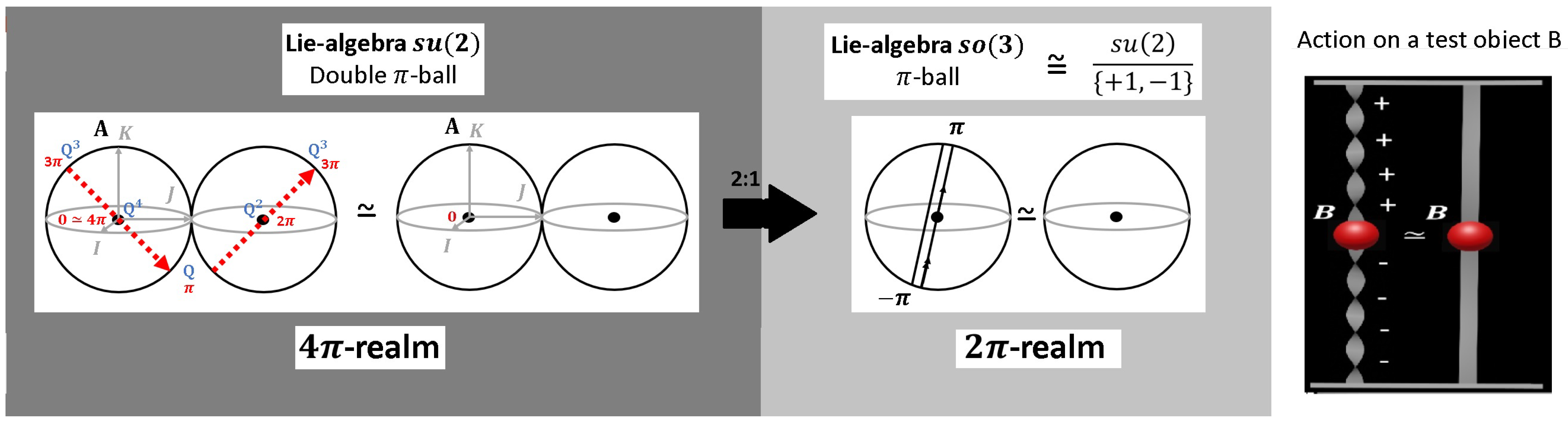
As a preparation, we are firstly going to discuss the geometric and topological properties of quaternions. As shown in detail in [10], geometrically, the group $SU\left(2\right)$ can be described in the Heegard-splitting by two $\pi$-balls (that is, volumes of two spheres with radius $\pi$), where the boundaries are identified. Transformations in these $\pi$-balls can be described by the quaternions

$$\begin{array}{c}\hfill I\equiv exp(-i\frac{\pi }{2}{\sigma }_x)=-i{\sigma }_x,J\equiv exp(-i\frac{\pi }{2}{\sigma }_y)=-i{\sigma }_y,K\equiv exp(-i\frac{\pi }{2}{\sigma }_z)=-i{\sigma }_z.\end{array}$$

(18)

In [4,10] a haptic model for the operations $I,J,K$ is introduced. In particular, the paths $IJK=-1$ and $JIK=+1$ are compared in Figure 3. The famous Dirac belt trick is shown in Figure 4. The $4\pi$-periodicity is reflected by $I^4=J^4=K^4=+1$.

Recently, the importance of the normed division algebras $\{\mathbb{R},\mathbb{C},\mathbb{H},\mathbb{O}\}$ for particle physics has been advocated by Furey [7]. In particular, within her framework, all of the Lorentz representations of the standard model can be described as generalized ideals within the algebra $\mathbb{C}\otimes \mathbb{H}$. Indeed, Equation (8) is a similar starting point, again leading to Lorentz representations with spin $\{a,b\}$. In this contribution, we wish to eplore more of the $topological$ consequences of this construction.

6. Knot Theoretic Description of the Dirac- and Maxwell Equations

Based on the four operations defined in (5) which emerge simply from a $distinction$, we found the basic building blocks

$$\begin{array}{c}\hfill \varphi \simeq {\sigma }_1,\varphi q\simeq -i{\sigma }_2,q\simeq {\sigma }_3,\pm id\end{array}$$

(19)

for any physical quantity. Thus, space-time $x_{\mu }{\sigma }^{\mu }$ naturally comes with a hermitian structure, and with all possible fields with $SU\left(2\right)\times SU\left(2\right)$ representations $(a,b)$ obeying a 2:1-mapping to space-time.

The most important examples to be discussed are the Weyl-spinors $(a,b)=(1/2,0)$ and $(a,b)=(0,1/2)$, the Dirac-spinor $(1/2,0)⨁(0,1/2)$, and the gauge field $A_{\mu }$$(1/2,1/2)$. In particular, the Maxwell-equations and the Dirac equation will follow just from these geometric properties.

In order to derive equations of motion, we introduce translations by replacing $(t,\overrightarrow{r})$ in (7) by $({\partial }_t,\overrightarrow{\nabla })$. In view of (10), we could define four types of operators $\pm (\pm {\partial }_t+\overrightarrow{\sigma }\overrightarrow{\nabla })$. As a global sign is irrelevant, we end up with two operators, related to each other by time reversal. In order to link to the usual notation of quaternions, and to their geometric interpretation as indicated in Figure 3, we scale with a factor $-i$ to define the differential operators

$$\begin{array}{c}\hfill {\mathbf{D}}_{+}\equiv +i{\partial }_0+I{\partial }_x+J{\partial }_y+K{\partial }_z\equiv +i{\partial }_t+\widehat{\nabla }\\ \hfill {\mathbf{D}}_{-}\equiv -i{\partial }_0+I{\partial }_x+J{\partial }_y+K{\partial }_z\equiv -i{\partial }_t+\widehat{\nabla }.\end{array}$$

(20)

Due to the commutation properties of quaternions, we find for the product

$$\begin{array}{c}\hfill {\mathbf{D}}_{+}{\mathbf{D}}_{-}={\mathbf{D}}_{-}{\mathbf{D}}_{+}={\partial }_0^2+{\widehat{\nabla }}^2=[{\partial }_t^2-{\overrightarrow{\nabla }}^2]\mathrm{id}+{[\overrightarrow{\nabla }\times \overrightarrow{\nabla }]}_k{Q}_k\end{array}$$

(21)

with $Q_k=(I,J,K)$ for $k=1,2,3$.

6.1. Weyl and Dirac Spinor Representations

The most straightforward way to operate with ${\mathbf{D}}_{\pm }$ is the fundamental representation. Let us introduce the complex spinors

$$\begin{array}{c}\hfill u_{+}\equiv \left[\begin{array}{c}{z}_1\\ z_2\end{array}\right],u_{-}\equiv \left[\begin{array}{c}-z_2^{*}\\ z_1^{*}.\end{array}\right]\end{array}$$

(22)

Geometrically, these spinors live in two separate hyperspheres $S_3$ with $|z_1{|}^2+{\left|z_2\right|}^2=1$. The equations of motions for the spinors with opposite chirality are then just given by ${\mathbf{D}}_{+}{u}_{+}=0,{\mathbf{D}}_{-}{u}_{-}=0$. This corresponds to the $(a,b)=(1/2,0)$ and $(a,b)=(0,1/2)$ representations of $SL(2,\mathbb{C})$. It is well known that $(2,1)$-torus knots emerge in the description of Weyl fields on $S_3$ [11,12]. Some explicit parameterizations can be found in, for example, [9]. A closed loop is reached after a $4\pi$-rotation induced by any quaternion Q after four inner twists, corresponding to $Q^4$. Positive and negative chiralities can be associated to one left or one right-twist in the $2\pi$-realm, which is topologically equivalent to four inner right twists $(++++)$ or four inner left twists $(----)$ in the $4\pi$-realm, see Figure 5. The Weyl spinor is the most prominent example for a $qubit$, representing the simplest quantum system. A common representation for the qubit is in the basis $|0\rangle$ and $|1\rangle$, corresponding to the complex vectors $(z_1,z_2)=(1,0)$ and $(z_1,z_2)=(0,1)$. In the $2\pi$-realm, the qubit is described on the Bloch sphere $S_2$. The Hopf-mapping $S_3\to S_2$ is given by

$$\begin{array}{ccc}\hfill \left(4\pi \right)-\mathrm{realm}& \to & \left(2\pi \right)-\mathrm{realm}\hfill \\ \hfill u_{+}\equiv (z_1,z_2)& \to & \overrightarrow{n}\equiv \left(u_{+}^{†}\overrightarrow{\sigma }{u}_{+}\right)=(\mathrm{Re}\left(2{\overline{z}}_1{z}_2\right),\mathrm{Im}\left(2{\overline{z}}_1{z}_2\right),|z_1{|}^2-|z_2{|}^2).\hfill \end{array}$$

(23)

In [10], we proposed to combine the Bloch-sphere representation with the paper strip model in order to distinguish the spin-flip operations $IJK=-IKJ$ as shown in Figure 3. Note, that the minus sign $-1=Q^2$ induces two additional inner twists.

Next, we turn to the Dirac equation, that is, the $(1/2,0)⨁(0,1/2)$ representation. In the chiral representation, the usual mathematical formalism leads to

$$\begin{array}{c}\hfill \left[\begin{array}{cc}-m& D_{-}\\ -D_{+}& -m\end{array}\right]\left[\begin{array}{c}{u}_{+}\\ u_{-}\end{array}\right]=0,\end{array}$$

(24)

which is just the Dirac equation $(i{\gamma }^{\mu }{\partial }_{\mu }-m)\psi =0$ with the four-components $\psi =(u_{+},u_{-})$ of the Dirac spinor. Here, m denotes the (bare) mass of the free Dirac spinor.

6.2. Maxwell’s Equations

So far, we discussed spinors, where the relation to quaternions and the 2:1-mapping from the $4\pi$-realm to the $2\pi$-realm is quite obvious. Here, we show explicitly that this construction can be repeated to find the equations of motion of electromagnetism. In order to do so, we introduce the time and spacial components of the gauge field as $A_{\mu }\equiv (A_0,\overrightarrow{A})$ in the language of quaternions, and introduce the field

$$\begin{array}{c}\hfill -i{A}_{\mu }{\sigma }^{\mu }=-i{A}_0+\widehat{A}\equiv -i{A}_0+A_{x}I+A_{y}J+A_{z}K.\end{array}$$

(25)

Acting with ${\mathbf{D}}_{-}$, we find

$$\begin{array}{c}\hfill {\mathbf{D}}_{-}(-i{A}_0+\widehat{A})=(-{\partial }_t{A}_0-\overrightarrow{\nabla }\overrightarrow{A})\mathbf{id}\\ \hfill +(-{\partial }_k{A}_0-{\partial }_0{A}_k)\mathbf{i}{\mathbf{Q}}_{\mathbf{k}}+{(\overrightarrow{\nabla }\times \overrightarrow{A})}_k{\mathbf{Q}}_{\mathbf{k}}\\ \hfill =\left[\mathrm{gauge}\mathrm{term}\right]\mathrm{id}+\mathrm{i}\widehat{\mathrm{E}}+\widehat{\mathrm{B}}\end{array}$$

(26)

and find the usual definition from the electric field $\overrightarrow{E}=-\overrightarrow{\nabla }{A}_0-{\partial }_0\overrightarrow{A}$ in the $iQ$-sector, and magnetic field $\overrightarrow{B}=\nabla \times \overrightarrow{A}$ in the Q-sector of the equation. The first term in the $\mathrm{id}$-sector can be set to zero in an appropriate gauge, and in any case, does not relate to observables, due to the gauge freedom

$$\begin{array}{ccc}\hfill \overrightarrow{B}& =& \overrightarrow{\nabla }\times \overrightarrow{A}=\overrightarrow{\nabla }\times (\overrightarrow{A}+\overrightarrow{\nabla }\Lambda )\hfill \\ \hfill \overrightarrow{E}& =& -\overrightarrow{\nabla }{A}_0-{\partial }_0\overrightarrow{A}=-\overrightarrow{\nabla }(A_0+{\partial }_0\Lambda )-{\partial }_0(\overrightarrow{A}-\overrightarrow{\nabla }\Lambda ).\hfill \end{array}$$

(27)

These gauge transformations can be combined to $A_{\mu }\to A_{\mu }-{\partial }_{\mu }{\Lambda }_{\mathrm{Maxwell}}$. If we introduce the charge density and the electric current in the quaternion language as $(-i\rho +\widehat{J})=(-i\rho \mathrm{id}+J_{x}I+J_{y}J+J_{z}K)$, then Maxwell’s equations follow from

$$\begin{array}{c}\hfill {\mathbf{D}}_{+}(\widehat{B}+i\widehat{E})=(-i\rho +\widehat{J})\end{array}$$

(28)

since in the four sectors proportional to $\mathbf{id}$, $i\mathbf{id}$, $\mathbf{Q}$, $i\mathbf{Q}$, we can read off Maxwell’s equations:

$$\begin{array}{c}\hfill \overrightarrow{\nabla }\overrightarrow{B}=0,\overrightarrow{\nabla }\overrightarrow{E}=\rho ,\overrightarrow{\nabla }\times \overrightarrow{B}-{\partial }_0\overrightarrow{E}=\overrightarrow{J},\overrightarrow{\nabla }\times \overrightarrow{E}+{\partial }_0\overrightarrow{B}=0.\end{array}$$

While Maxwell’s starting point has been evidence collected in experimental physics, the starting point introduced here is axiomatic and based on a $distinction$ as introduced in Section 3, and on group theory. Although quaternions have been introduced already in 1843 by Sir Hamilton, a contemporary of Maxwell, their fundamental importance in physics became only evident much later—with the advent of quantum physics.

Crucially, the gauge transformation induces the transition between topologically equivalent configurations in the $4\pi$-realm, with no observable effect in the $2\pi$-realm. From a mathematical point of view, this means that gauge fields within the same cohomology class lead to identical observables. The genius 19th century physicists Maxwell himself did already know this equation in the framework of classical electromagnetism. However, Maxwell did not know spin $1/2$-fields, and the corresponding transformation ${\psi }_{\Lambda }\to e^{i{\tilde{\Lambda }}_{\mathrm{Dirac}}}\psi .$ In quantum physics, the scalar field ${\tilde{\Lambda }}_{\mathrm{Dirac}}$ is unobservable due to $|e^{i{\tilde{\Lambda }}_{\mathrm{Dirac}}}{|}^2=1$ in the $2\pi$-realm. However, in the $4\pi$-realm, infinitely many topologically identical configurations are associated to this single observable. Minimal interaction between the gauge field and the spin $1/2$-field is derived by $identifying$ the irrelevant phase ${\tilde{\Lambda }}_{\mathrm{Dirac}}$ of the spin $1/2$-field with the unobservable gauge freedom of the electric and magnetic field, ${\Lambda }_{\mathrm{Maxwell}}={\tilde{\Lambda }}_{Dirac}$. This is the starting point of gauge theory.

The key point we want to make is that the 2:1-mapping from the $\left(4\pi \right)$-realm to the $\left(2\pi \right)$-realm seems to be essential for all kinds of observable fields. In particular, $closed$ homotopic loops can be interpreted to encode spin j-representations, see Figure 5 (and Section 7.2). For spin $j=1/2$, a closed Dirac belt with $4j+2=4$ inner twists in the $4\pi$-realm is equivalent to a Moebius strip with one twist in the $2\pi$-realm. Due to the symmetry of the 2:1-mapping from $SL(2,\mathbb{C})$ to $SO(3,1)$, the paper strip must be closed to a torus as shown in Figure 2. In terms of Dehn twists in the $2\pi$-realm, if we start with a torus in the $2\pi$-realm, cut it open, make a $\pi$-rotation, and re-glue the torus, we obtain a Klein bottle.

For spin $j=1$, respectively, in terms of Dehn twists, we start with a torus in the $2\pi$-realm, cut it open, make a $2\pi$-rotation, and re-glue the torus. Again, we can model this operation using a paper strip, introducing two twists. Note, that a $2\pi$-Dehn twist corresponds by definition to a full rotation, that is, two twists in the paper strip. The merit we gain from the paper strip is that we can translate this configuration back to the $4\pi$-realm by cutting the paper strip open to find a Hopf link as shown in Figure 5 as the corresponding topology of the $j=1$-quantum state in Hilbert space.

In general, in the $2\pi$-realm, a torus with j Dehn twists corresponds to a SU(2)-representation with spin j. Equivalently, in the $4\pi$-realm, this corresponds to $4j+2$ inner twists (fermions; j = half-integer), and $2j+2j$ inner twists (bosons; j = integer), respectively [13].

In [5], we apply this haptic model for minimal interaction in some explicit examples, for example, the derivation of selection rules in atomic physics. Here, in the following section, we discuss the interaction of two and more qubits within the same framework and discuss the role of entanglement as the counterpart to a distinction.

7. How to Undo a Distinction: Haptic Model for Entanglement

7.1. Entanglement of Two Qubits

It is a reasonable and at the same time fascinating idea to start with $nothing$, in other words, with the unknot. In the $2\pi$-realm, consider a simple torus without any twists, see Figure 2. We introduce a $virtual$ twist into this torus in the following sense: While a Dehn twist is usually defined by the operations (1) cut the torus open (2) insert a rotation by the angle $\alpha =2\pi$ (3) re-glue the torus, a $virtual$ Dehn twist only amounts to the operation (2). In such a way, when applying all kinds of virtual Dehn twists, we obtain infinitely many topologically equivalent configurations which are all omnipresent within nothing. Once we cut the torus open twice and re-glue to obtain two independent tori, we ‘create’ particles—in other words, we distinguish certain topological configurations from each other.

In Figure 6, we show pair creation using this novel ansatz. We introduce a virtual $\pi$-Dehn twist into the original torus without cutting it open. This configuration can be interpreted as a superposition of two spin $1/2$-fields, that is, an entangled Bell-state

$$\begin{array}{c}\hfill |{\mathsf{\Psi }}^{+}\rangle =\frac{1}{\sqrt{2}}\left(\right|0_A{1}_B\rangle +|1_B{0}_A\rangle .\end{array}$$

(29)

Using the paper strip model (by cutting the torus open), we arrive at the simple haptic model shown in Figure 1 with the topologically equivalent configurations $\{\varnothing ,RL,LR\}$ (that is, a torus without any virtual twists and with a virtual $\pi$-Dehn twist). In Figure 4, we show the corresponding topologically equivalent configurations $\left\{\varnothing \right\},\{++++----\},\{----++++\}$ in the $4\pi$-realm. Particle creation in the $4\pi$-realm corresponds the transition of the trivial topology to two opposite Dirac belts as shown in Figure 7:

$$\left\{\varnothing \right\}\to \left\{\right(++++),(----\left)\right\}.$$

The transition from the entangled state to a mixed state of distinguishable particles is (formally) achieved by taking the partial trace,

$$\begin{array}{c}\hfill {\mathrm{tr}}_A|\psi \rangle \langle \psi |=\frac{1}{2}\left[\right|0_B\rangle \langle 0_B|+|1_B\rangle \langle 1_B\left|\right].\end{array}$$

(30)

Topologically, identification of the edges of the Dirac belts and identification of the parts $(0,2\pi )$ and $(2\pi ,4\pi )$ as shown in Figure 5 leads to two opposite Klein Bottles.

Reversely, both Klein Bottles can merge again to the unknot as shown in Figure 6. This corresponds to the superposition of two (indistinguishable) particles to an entangled state.

We conclude that it is reasonable to assume that the entanglement of a quantum state increases when the number possibilities to make distinctions decreases. Intuitively speaking, the $unknot$ has in some sense the largest amount of entanglement, as no distinction whatsoever can be made—even the number of qubits remains unclear unless we specify which of the topologically equivalent configurations we want to consider. In Section 7.4, we explore the concept of $virtual$ Dehn twists further to model entanglement more in detail.

7.2. Explicit Model for Interactions and Entanglement of Two Qubits

In order to link the topological model proposed in the last section to the dynamics in Hilbert space, we consider as an explicit example two distinct qubits $(A,B)$ as an initial state. We may write a general product state as

$$\begin{array}{c}\hfill |A\rangle |B\rangle =\left(z_1\right|0\rangle +z_2|1\rangle )\left(w_1\right|0\rangle +w_2|1\rangle ).\end{array}$$

(31)

This kind of state results from the mathematics derived from a distinction, with the local transformation group $SU\left(2\right)\times SU\left(2\right)$. However, the full unitary transformation group for two qubits is $U\left(2^2\right)=U\left(4\right)$. The complement $U\left(4\right)/\left(U\right(2)\times U(2\left)\right)$ describes non-local transformations (from the perspective of the $2\pi$-realm), and indeed, defines all possible interactions between the qubits. These non-local operations undo distinctions and lead to entanglement, as we show in what follows. For example, let us consider the Ising-type Hamiltonian $H=\hslash \omega (K\times K)$. Unitary time development is given by

$$\begin{array}{c}\hfill |\psi \left(t\right)\rangle =exp\left[i\omega t\right(K\times K\left)\right]|{+}_A\rangle |{+}_B\rangle =\frac{1}{2}[e^{+it\omega }\left(\right|00\rangle |+|11\rangle \left|\right)+e^{-it\omega }\left(\right|01\rangle |+|10\rangle \left|\right)].\end{array}$$

(32)

This time development describes periodic oscillation between the distinguishable state $\psi \left(0\right)=|{+}_A\rangle |{+}_B\rangle$ to the Bell state

$$\begin{array}{c}\hfill \psi (\pi /\left(4\omega \right))=\frac{1}{\sqrt{2}}\left(\right|0_{\alpha ,A}{1}_{\alpha ,B}\rangle +|1_{\alpha ,B}{0}_{\alpha ,A}\rangle \end{array}$$

(33)

$$\begin{array}{ccc}\hfill |0_{\alpha }\rangle & =& +cos(\pi /8)e^{-i\pi /4}|0\rangle +sin(\pi /8)e^{+i\pi /4}|1\rangle \hfill \\ \hfill |1_{\alpha }\rangle & =& -sin(\pi /8)e^{-i\pi /4}|0\rangle +cos(\pi /8)e^{+i\pi /4}|1\rangle .\hfill \end{array}$$

We may track the degree of entanglement by the so-called concurrence [14], given by $c=2|z_{00}{z}_{11}-z_{01}{z}_{10}|$ for a general pure two qubit state ${\sum }_{i,j\in 0,1}{z}_{ij}|ij\rangle$. Geometrically, this is just $S^7$. For $c=0$, we have a product state within two separate Bloch spheres $S_2\times S_2$; the Bell states are maximally entangled with $c=1$ and form an $\mathbb{R}{P}^3$. In the case at hand, the concurrence is given by

$$\begin{array}{c}\hfill c=|sin(2\omega t\left)\right|.\end{array}$$

(34)

For fixed c, we have five-dimensional, fixed submanifolds with given degree entanglement [15]. Any kind of interaction in a two-qubit system leads to such an oscillation between separable states with $c=0$ and maximally entangled states with $c=1$. It depends on the type of interaction which path within $S^7$ is chosen between the submanifolds $c=0$ and $c=1$, and which kind of states ($A,B)$ will be separable. For simplicity of the notation, we redefine $\left\{\right|0_{\alpha }\rangle ,|1_{\alpha }\rangle \}$ to $\left\{\right|0\rangle ,|1\rangle \}$ in what follows. Taking the trace over one qubit, we find

$$\begin{array}{c}\hfill {\mathrm{tr}}_A|\psi \rangle \langle \psi |=\frac{1}{2}\left[\right|0_B\rangle \langle 0_B|+|1_B\rangle \langle 1_B|.\end{array}$$

Just as is evident from the simple haptic model introduced in Section 2, the association of B to the configurations $|0\rangle$, $|1\rangle$ is random simply because before making the distinction $(A,B)$, the configurations $|0\rangle$, $|1\rangle$ did not exist separately, but have been part of the entangled state as shown in Figure 7 in the $\left(2\pi \right)$-realm, and as well in Figure 7 in the $\left(4\pi \right)$-realm (Hilbert space).

There is no elegant way to model the full time development (32) just with Dehn twists, as the knot representation of the entangled state depends on the chosen homotopic loop. Only if the homotopic loop is chosen appropriately, the initial state $\psi \left(0\right)$ and the Bell state $\psi (\pi /(4\omega \left)\right)$ have a simple representation, which can be read off from Figure 8. As the complexity of the mathematical structure cannot be undone just be changing the representation, this is no surprise. In the next section, we take advantage of this fact to give a more detailed interpretation of the relation between the knot structure and the corresponding amplitudes of the qubit in Hilbert space.

7.3. Homotopic Loops

Knot theory is in no way a different—or an alternative approach—to quantum physics. Rather, amplitudes in Hilbert space naturally incorporate knot structures. Note, that only within $S_3$ (corresponding to a single quantum state with spin $|j,m\rangle$), we may speak of knots, as in dimension $d\ge 4$, all knots become trivial. Thus, these knots arise as boundaries of higher dimensional manifolds.

We may extend the Hilbert space ${\mathbb{C}}^2$ for $j=1/2$ to ${\mathbb{C}}^{2j+1}$, introducing the homogeneous coordinates $Z_0,Z_2,\dots Z_{2j}$. For $SU\left(2\right)$-representations, the full hypersphere $S^{4j+1}$ of possible quantum states is not explored (this would be the orbit of a pure state rotated by the full group $U(2j+1)$). Rather, following Kramer [15], the submanifold where $S_3$ is wrapped $2j$ times onto itself leads to a representation of the spin j state in the Hilbert space, with homogeneous coordinates $Z_k$ $(k=0,\dots 2j)$ given by:

$$\begin{array}{c}\hfill Z_k={\left(\genfrac{}{}{0pt}{}{2j}{k}\right)}^{-1/2}{z}_1^k{z}_2^{2j-k}.\end{array}$$

(35)

Equation (35) defines a $\left(2j\right)$-to-one mapping $S_3\to S_3$ with $\left(\right|z_1{|}^2+|z_2{\left|\right)}^{2j}={\sum }_{k=0}^{2j}{Z}_k^{*}{Z}_k$. In other words, spin j-representations in Hilbert space can be seen as three-dimensional manifolds obtained by a certain mapping of $S_3$ onto itself. (Framed) braids are obtained as certain boundaries of these manifolds. After Hopf mapping $S_3\to S_2$, we obtain in the so-called stellar representation a polynomial of a single complex variable with degree $2j$ [12]. In general, the position of these nodes can be rotated to arbitrary locations on the Bloch sphere. In Figure 11, the position of the corresponding $2j$ nodes is indicated by crosses on the Bloch-sphere (after stereographic projection of the complex plane to $S_2$). An even number of $2l$ nodes can equivalently be represented by l nodal lines, leading to the spherical harmonics shown in Figure 8.

We consider a single qubit, the singlet and triplet state as explicit examples. In the usual notation for spin $|j,m\rangle$, these states are given by

$$\begin{array}{ccc}\hfill |1,-1\rangle =|00\rangle ,|1,0\rangle =\frac{1}{\sqrt{2}}\left(\right|01\rangle & +& |10\rangle ),|1,1\rangle =|11\rangle \hfill \\ \hfill |\frac{1}{2},-\frac{1}{2}\rangle =|0\rangle & ,& |\frac{1}{2},\frac{1}{2}\rangle =|1\rangle \hfill \\ \hfill |0,0\rangle =\frac{1}{\sqrt{2}}\left(\right|01\rangle & -& |10\rangle ).\hfill \end{array}$$

(36)

This construction may be extended to any spin j-state. These states have many different applications, from atomic physics to quantum information theory. Thus, these states are represented in various manners, ranging from (s-/p-) orbitals of an atom to entangled qubits in a circuit for a quantum computer. While in atomic physics, usually only the Bloch-sphere representation is considered, here, we want to exploit the knot structures in Hilbert space on certain homotopic loops. If all homotopic loops are combined, we arrive at a representation of the qubits as a manifold as indicated above.

For the $4\pi$-realm, we show in Figure 8 the knot structure emerging up to spin $j=1$ for two different homotopic loops: A rotation around the z-axis, and a rotation around the x-axis. Note, that a double traversal of the Bloch sphere is necessary in order to close the loop in Hilbert space. Explicitly, we discuss the Bell state

$$\begin{array}{c}\hfill |1,0\rangle =\frac{1}{\sqrt{2}}\left(\right|01\rangle +|10\rangle =\frac{1}{\sqrt{2}}\left(\right|++\rangle -|--\rangle ).\end{array}$$

(37)

First, we consider the homotopic loop defined by a $0\le \vartheta \le 4\pi$ rotation in z-direction, and find that the phase remains constant, since

$$\begin{array}{c}\hfill (e^{i\frac{\vartheta }{2}{\sigma }_z}\times e^{i\frac{\vartheta }{2}{\sigma }_z})\frac{1}{\sqrt{2}}\left(\right|01\rangle +|10\rangle )=\frac{1}{\sqrt{2}}\left(\right|01\rangle +|10\rangle ).\end{array}$$

(38)

Next, we consider the homotopic loop in x-direction, leading to

$$\begin{array}{c}\hfill (e^{i\frac{\vartheta }{2}{\sigma }_x}\times e^{i\frac{\vartheta }{2}{\sigma }_x})\frac{1}{\sqrt{2}}\left(\right|++\rangle -|--\rangle )=\frac{1}{\sqrt{2}}\left(e^{i\vartheta }\right|++\rangle -e^{-i\vartheta }|--\rangle ).\end{array}$$

(39)

The corresponding knot structure for these homotopic loops is shown in Figure 8. We can see that the Bell state $|1,0\rangle$ already shows two different characteristics depending on the homotopic loop considered: The z-loop is characterized by a superposition of homotopically equivalent configurations—related to each other via permutations. The x-loop is characterized by a superposition of homotopically non-equivalent configurations, related to $nodes$ in the $2\pi$-realm hit by the homotopic loop. Note, that two nodes are equivalently described by one nodal line (in other words, the spherical harmonics $Y_{1m}$ has one nodal line $l=1$, which can be constructed by two single qubits with one node each [15].

Next, we discuss the topological interpretation of the ladder operators $L^{\pm }$ of the angular momentum algebra $[L_z,L^{\pm }]=\pm i\hslash L_{\pm }$, $[L^{+},L^{-}]=2\hslash L_z$. Starting with the Bloch sphere-scenario, we see that $L^{\pm }$ manipulates the position of the $2j$ nodes, but does not change its total number.

For $j=1/2$, we may rewrite $L^{\pm }$ in quaternion language as $L^{\pm }\to -\frac{1}{2}(I\pm iJ)$. The effect of this operation on a knot is a reversal of the sign of the node in the K-homotopy (that is, rotation around the z-axis). For the corresponding Dirac belt, the inner twists are changed as $(++++)\to (----)$. Note that the effect of the ladder operator is $not$ a change of the topology, as the total number of nodes remains unchanged. Only the position of the nodes is changed as shown in Figure 8.

Topological changes as described by the unitary time evolution (32) are only possible when non-local operations—in this example, $H=\omega (K\times K)$, with $e^{-iHt/\hslash }\in U\left(4\right)/$$\left(U\right(2)\times U(2\left)\right)$—act on a given initial state. In Figure 9, we show the corresponding knot structure in those homotopic loops where $\left|\psi \right(t)\rangle$ has a simple structure (compare also to Figure 8 for the corresponding knots at different homotopic loops).

7.4. Entanglement of Three Qubits

In what follows, we consider entanglement of multiple qubit systems, starting with three qubits. In Section 7.1, we argued that the $unknot$ corresponds to an entangled state, as no distinction whatsoever can be made. However, note that the question which state has the largest entanglement is a highly non-trivial question, as even the measure for the “degree of entanglement” is not uniquely defined for more than two qubits. One way to describe entanglement in a composite systems is to consider some of its bipartitions and to average over certain entanglement measures. For a review, we refer to [16].

For an odd number of qubits, the starting configuration cannot be the unknot, but R (or L). Note that R is topologically equivalent to $RLR,RRL,LRR$ using virtual Dehn twists as introduced in Section 7.1. For three qubits, this superposition of permutations just leads to the $|W\rangle$-sate, given by [17]

$$\begin{array}{c}\hfill |W\rangle =\frac{1}{\sqrt{3}}\left[\right|001\rangle +|010\rangle +|100\rangle ].\end{array}$$

(40)

In Figure 10, we show the corresponding knots for the z-homotopy.

Taking the partial trace, we find

$$\begin{array}{c}\hfill {\mathrm{tr}}_A|W\rangle \langle W|=\frac{2}{3}|{\mathsf{\Psi }}^{+}\rangle \langle {\mathsf{\Psi }}^{+}|+\frac{1}{3}|00\rangle \langle 00|,\end{array}$$

(41)

with the Bell state $|{\mathsf{\Psi }}^{+}\rangle =\frac{1}{\sqrt{2}}\left[\right|01\rangle +|10\rangle ]$. As shown in Figure 10, this result can directly be read off from the knot structure without calculation. Once again, randomness emerges due to the fact that before taking the trace, there is no qubit A from a topological point of view. Rather, in order to make the distinction between three qubits, three labels $(A,B,C)$ must be distributed to the topologically equivalent knot configurations $\{RRL,RLR,LRR\}$, which is by construction arbitrary.

The GHZ-state $|GHZ\rangle =\frac{1}{\sqrt{2}}\left[\right|000\rangle +|111\rangle ]$, on the other side, is the superposition of topologically opposite configurations as shown in Figure 11. Note, that the $|W\rangle$ and $|GHZ\rangle$ state follow as straightforward generalizations of the two homotopic loops of the state $|1,0\rangle$ shown in Figure 8. Taking the partial trace, we find

$$\begin{array}{c}\hfill {\mathrm{tr}}_A|GHZ\rangle \langle GHZ|=\frac{1}{2}|00\rangle \langle 00|+\frac{1}{2}|11\rangle \langle 11|,\end{array}$$

(42)

which is just a mixture without remaining entanglement. Among all three-qubit pure states, the genuine three-party entanglement measured by the three-tangle [18] is largest for the state $|GHZ\rangle$, while the two-tangle and the $persistence$ of entanglement [19] has its maximum for the state $|W\rangle$.

7.5. (Generalized) HS-States

In case of four qubits, by application of a virtual $\left(2\pi \right)$-Dehn twist to the unknot, we find $RRLL$. There are in total six permutations, and thus we arrive at the superposition of all these configurations for the entangled state. Any such permutation can be seen as a combination of virtual Dehn twists at different locations of the torus. In similar vein, each permutation $\Pi$ can be expressed as combination of single transpositions ${\pi }_{ij}$ at positions $i,j$. We introduce the inverse transposition as ${\pi }_{ij}{\pi }_{ij}^{-1}={\pi }_{ij}{\pi }_{ji}=1$. We may assume that a transposition changes the phase of the quantum state by a factor $w\equiv e^{2\pi ib}$. We introduce the so-called Higuchi-Sudbery states of four qubits as [20]

$$\begin{array}{ccc}\hfill |{\mathrm{HS}}_a\rangle & =& \frac{1}{\sqrt{6}}[\left(\right|0011\rangle +|1100\rangle )+w\left(\right|0101\rangle +|1010\rangle )+w^2\left(\right|0110\rangle +|1001\rangle )]\hfill \\ & \equiv & \frac{1}{\sqrt{6}}[\left(\right|A\rangle +w|B\rangle +w^2|C\rangle ]\hfill \\ \hfill |{\mathrm{HS}}_b\rangle & \equiv & \frac{1}{\sqrt{6}}[\left(\right|A\rangle +w|C\rangle +w^2|B\rangle ].\hfill \end{array}$$

(43)

Thus, we find a doublet with respect to the transposition ${\pi }_{12}$, since ${\pi }_{12}|{\mathrm{HS}}_a\rangle =\omega |{\mathrm{HS}}_b\rangle$ and ${\pi }_{12}|{\mathrm{HS}}_b\rangle =\omega |{\mathrm{HS}}_a\rangle$. At first, the phase w is arbitrary. As shown in the appendix, for $w^3=e^{2\pi i}$, the entropy of entanglement averaged over all bipartitions becomes maximal. Indeed, in this case, the states $\left\{\right|{\mathrm{HS}}_a\rangle ,|{\mathrm{HS}}_b\rangle \}$ are not only a doublet with respect to ${\pi }_{12}$, but to $any$ transposition ${\pi }_{ij}$.

However, also for $w^3=e^{\pi i}=-1$, the entanglement entropy is maximal, while the generalized HS-state is only a doublet with respect to the transposition ${\pi }_{12}$. In general, for more than four qubits, doublets with $w\ne 1$ can be constructed only for $one$ given transposition. In this sense, the construction made by Higuchi and Sudbery for the four-qubit case is unique. For $w=1$, this state is equivalent to the Dicke state $D_4^{\left(2\right)}$, which will be discussed in the next section.

7.6. Dicke States

In case of six qubits, we can insert a virtual $\left(3\pi \right)$-Dehn twist by rotating the torus around itself with the angle $3\pi$ to find $RRRLLL$. There are in total 20 permutations, and thus we arrive at the superposition of all these configurations. In general, in case of l insertions of R-twists and $(N-l)$ insertions of L-twists, summation over all topologically equivalent configurations leads to the so-called Dicke state

$$\begin{array}{c}\hfill |D_N^{\left(l\right)}\rangle ={\left(\genfrac{}{}{0pt}{}{N}{l}\right)}^{-1/2}\sum _{\Pi }{\Pi }_i\left(\right|R^{\otimes l}{L}^{\otimes N-l}\rangle ).\end{array}$$

(44)

The superposition of all topologically equivalent configurations signifies that the state is close to trivial topology, that is, the unknot. Thus, just using the concept of virtual Dehn twists, it is reasonable to assume that entanglement is maximally persistent and robust under particle losses, as all configurations are related to all others by single transpositions.

Experimental evidence for this characteristic trait of Dicke states has been gathered in several experiments. As an example, Wieczoreck et al. [21] describe an experimental scheme to produce the six-photon Dicke state $D_6^{\left(3\right)}$ by means of spontaneous parametric down-conversion. As photons have spin 1, we have to think of a virtual $\left(6\pi \right)$-Dehn twist in Equation (44), which amounts in reinterpretation of R as a $\left(2\pi \right)$-rotation rather than the $\pi$-rotation corresponding to a spin $1/2$-qubit. After the authors have shown that the produced six-photon state comes close to the ideal Dicke state $D_6^{\left(3\right)}$ by performing coincidence measurements and determining benchmark parameters such as state fidelity and expectation values of witness-operators, they proceed to test whether entanglement is preserved under different local projections and, specifically, under loss of one qubit. Tracing out one qubit from the state corresponds to the transition of the six-photon Dicke state into a mixture of two five-photon Dicke states:

$$\begin{array}{c}\hfill |D_6^{\left(3\right)}\rangle \underrightarrow{{}^{\mathrm{partialtrace}}}\frac{1}{2}\left(|D_5^{\left(2\right)}\rangle \langle D_5^{\left(2\right)}|+|D_5^{\left(3\right)}\rangle \langle D_5^{\left(3\right)}|\right).\end{array}$$

(45)

Since the obtained mixture again consists of five-qubit Dicke states, entanglement is still present after one qubit is lost. Indeed, this state emerges from $RRRLLL$ after one R $or$ L is crossed out.

The measurement of entanglement by means of witness operators performed in [21] revealed that the experimentally created state indeed preserves entanglement under particle loss, as can be expected from Equation (45). Other experiments have been conducted that show the remarkable properties of Dicke states in a similar fashion [22,23].

To conclude, we find that indeed, the unknot is intimately related to entanglement, which is particularly robust under particle loss, as shown for the W-state (three qubits), the $HS$-state (four qubits, and in general for Dicke states (N qubits).

In the next section, we show how the state $RRRLLL$ can be modeled using virtual Dehn twists, and compare our model for the transition to a mixed state with a mathematical model introduced by Kauffmann.

7.7. The Kauffmann Model

Reassuringly, the topological model for the relation between entanglement, distinctions and quantum randomness shown in Figure 7 is also consistent with a conjecture made by Kauffmann [4]. He proposed a knot theoretic ansatz for interactions between qubits based on algebraic topology [4].

In general, a $(p,q)$-torus knot is described by the singular boundary defined by $\mathbf{K}=\left\{(z_1,z_2)\right|z_1^p+z_2^q=0,|z_1{|}^2+|z_2{|}^2=1\}$.

The threefoil knot corresponds to the case $(p,q)=(3,2)$. It is a general result that a pair of complementary knots can be created from the unknot. In case of the $(3,2)$-torus knot, we may extend the algebraic description to [4,24]

$$\begin{array}{c}\hfill {\Sigma }^7\left(K\right)=\left\{(z_i,\in S^9,i=1\dots 5)\right|z_1^3+z_2^3+(z_3^2+z_4^2+z_5^2)=0,\\ \hfill |z_1{|}^2+|z_2{|}^2+|z_3{|}^2+|z_4{|}^2+|z_5{|}^2=1\}\end{array}$$

(46)

and follow the “birth” and “death” of the $(3,2)$ torus knot K within the hypersphere $S^9$ [24].

In Figure 12, we compare this ansatz for the creation of a pair of $(3,2)$-torus knots from an unknot with the model of virtual Dehn twists. From the point of view of physics, $(2j,2)$ torus knots can be associated with a spin j-representation [11,13]. Within the model of virtual Dehn twists, we can reproduce these results in the following manner: We represent the torus in the $2\pi$-realm using a simple paper strip as shown in Figure 2, assuming that the edges are identified. Starting with the unknot, insert three rotations to obtain the topologically equivalent configuration $RRRLLL$. Just repeating the same steps as in the two-qubit case (Figure 7), including the torus splitting, here, we obtain two $(3,2)$-torus knots with eight inner twists of opposite sign. The haptic model for the transition reproduces the creation of two torus knots as proposed by Kauffmann. Note that the 2:1-mapping is not done in Kauffmann’s ansatz explicitly. Using the paper strip model in the $4\pi$-realm, we rearrange the $(3,2)$-torus knots to obtain a state with just three twists $RRR$, $LLL$ in the $2\pi$-realm, corresponding to the transition of the entangled state $|G_6\rangle \equiv \frac{1}{\sqrt{2}}\left(\right|000\rangle |111\rangle +|111\rangle |000\rangle )$ to the distinct product states ${\mathrm{tr}}_{123}|G_6\rangle \langle G_6|=\frac{1}{2}\left[\right|{000}_A\rangle \langle {000}_A|+|{111}_B\rangle \langle {111}_B|$. Our topological model for the origin of quantum randomness remains also valid for this situation, since within the entangled state, the distinct knots A and B are in a superposition and merge to an unknot with trivial topology.

Note, that the entanglement of the state created by the twist $RRRLLL$ is not robust, as it is of the type of a GHZ-state. Entanglement which is robust against particle loss is obtained when all possible permutations within $RRRLLL$ are in superposition $|D_6^3\rangle$ (44). In this sense, the Dicke state is a generalization of the W-state rather than the $GHZ$-state.

8. From Quaternions to Octonions: Normed Division Algebras and $\mathit{SU}\left(\mathbf{3}\right)$

8.1. Modeling Color Confinement and $SU\left(3\right)$ with Virtual Dehn Twists

Although many more knot structures beyond these simple $(a,b)$-representations can be imagined, in fact, within the standard model, no other observables exist. For example, the color degree of freedom with underlying $SU\left(3\right)$-gauge symmetry does not match this pattern, and is $confined$ to singlet states.

Let $|q_i\rangle$ ($i=1,2,3$) be the i-th color of the quark, then a Baryon must be in the color singlet state given by

$$\begin{array}{c}\hfill |B\rangle =\frac{1}{\sqrt{3!}}{ϵ}_{ijk}|q_i{q}_j{q}_k\rangle =\frac{1}{\sqrt{3}}\left[\right|q_1\rangle |{\mathsf{\Psi }}^{-}{\rangle }_{23}+|q_2\rangle |{\mathsf{\Psi }}^{-}{\rangle }_{31}+|q_3\rangle |{\mathsf{\Psi }}^{-}{\rangle }_{12}].\end{array}$$

(47)

Indeed, a $U\left(3\right)$-rotation in color space leaves this configuration invariant. We rewrite this expression using the antisymmetric Bell state $|{\mathsf{\Psi }}^{-}{\rangle }_{ij}=1/\sqrt{2}\left(\right|q_i\rangle |q_j\rangle -|q_j\rangle |q_i\rangle )$. We introduce virtual Dehn twists with a $\pi /3$-rotation as shown in Figure 13. A combination of three quarks can be modeled by a virtual Dehn twist with rotation angle $\pi$, which in the notation introduced in the previous sections amounts to $RL$. However, in contrast to $SU\left(2\right)$-representations which can be modeled with two framed braids, here, we encounter three (cylic) framed braids, see also Figure 14. Interestingly, the knot structure encountered in the $RL$-braid with three strands automatically reproduces Equation (47), as shown in Figure 13. For $SU\left(3\right)$, the mapping to observables is 3:1, and thus only the combination (47) can be observed.

Concerning mesons, the equation

$$\begin{array}{c}\hfill |M\rangle =\frac{1}{\sqrt{3}}\left(\right|q_r{\overline{q}}_r\rangle +|q_g{\overline{q}}_g\rangle +|q_b{\overline{q}}_b\rangle )\end{array}$$

(48)

encodes a superposition of the three ‘colors’ and ‘anti-colors’ $i=1,2,3\equiv r,g,b$. Each term for itself corresponds to a virtual Dehn twist with rotation angle $\pi$. As any color is part of the superposition, we can think of this configuration as three adjacent twists ${\left(RL\right)}^3$ in a superposition of all permutations, that is, the Dicke state $|D_6^{\left(3\right)}\rangle$ as defined in (44). However, in contrast to the situation described in Section 7.7 with $SU\left(2\right)$-representations which can be modeled with two framed braids, here, we once again encounter three (cyclic) framed baids. Indeed, this configuration can be viewed as any of the color-anticolor pairs. For example, using a Reidemeister move, we may rearrange

$$\begin{array}{c}\hfill \left(RL\right)\left(RL\right)\left(RL\right)\simeq \left(ABAaba\right)\left(ABAaba\right)\left(ABAaba\right)\simeq AB\left(Ab\right)abBA\left(Ba\right)baABAaba\simeq \left(Ab\right)\left(Ba\right),\end{array}$$

(49)

which encodes the green-antigreen pair $\left(Ab\right)\left(Ba\right)$. Note, that for a single color state, the 3:1 mapping is impossible. For example, the configuration $Ab$ corresponds—after torus splitting—to a single loop with 6 inner twists, which does not allow for a re-gluing, as can easily be checked using the haptic model proposed in Figure 13. But even the configuration $\left(Ab\right)\left(Ba\right)$ cannot exist ‘alone’: The 3:1-mapping is only possible via the construction of virtual Dehn twists: Only those knots which emerge by virtual Dehn twists can become free particles via torus splitting. In this sense, the configuration $\left(Ab\right)\left(Ba\right)$ cannot exist without coexistence of the other color/anti-color pairs $\left(Ab\right)\left(Ba\right)$ and $\left(ab\right)\left(BA\right)$, as they are part of the virtual Dehn twist ${\left(RL\right)}^3$ (49), which indeed is a color singulet.

We conclude that the extension of the construction of virtual Dehn twists from $SU\left(2\right)$ to $SU\left(3\right)$ is possible and can be modeled using three framed braids. For $SU\left(2\right)$, all spin j-states can be obtained via virtual Dehn twists and torus splitting, and lead to observables. In sharp contrast, for $SU\left(3\right)$, only color singulet states can be mapped to observables, as described above.

Due to the complexity of the problem of color confinement, of course we do not claim to be able to have a proof of it. Rather, we made a consistency check to the statement that those knots related to observables must be part of $(a,b)$-representations of the Lorentz group and match the conditions for the mapping to space-time. In case of the gauge group $SU\left(3\right)$, this is only possible for singulets within our model.

8.2. Normed Division Algebras

While virtual Dehn twists seem to be a valid tool to model particles, in this section, we want to compare our ansatz with other topological approaches to particle physics.

As discussed in Section 5, recently, the normed divison algebras $\{\mathbb{R},\mathbb{C},\mathbb{H},\mathbb{O}\}$ have been introduced to model the particle content and symmetries within the standard model [7]. As shown in Figure 14, we may visualize all normed division algebras as a Fano Cube: Starting with the real numbers $\mathbb{R}$, the complex unit i allows for the extension to the complex numbers $\mathbb{C}$, while the introduction of the quaternions $I,J,K$ within $SU\left(2\right)$ as defined in (18) leads to the algebra $\mathbb{H}$. Four dimensional space-time (16) as derived from a distinction in Section 3 corresponds to the part $\mathbb{R}\otimes \mathbb{H}$ of the algebra, while Lorentzian degrees of freedom are related to $\mathbb{C}\otimes \mathbb{H}$, that is, the covering group $SL(2,\mathbb{C})$ of $SO(3,1)$, see Equation (8). All known particles in the standard model fall into this category as $(a,b)$-representations of $SU\left(2\right)\times SU\left(2\right)$.

Octonions are introduced by one additional generator L, which completes the set of generators of quaternions $(1,I,J,K)$ to those of the octonions: $e_i,i=1,\dots 8$ given by $(1,I,J,K,L,IL,JL,KL)$. According to Furey, the part $\mathbb{C}\otimes \mathbb{O}$ can be associated to internal degrees of freedom, such as color, weak isospin, and charge [7]. In particular, the group $SU\left(3\right)$ is the subgroup of the special group $G_2$ of automorphims of the octonions which fixes one given octonion.

The relation between normed division algebras, braids and the Preon model has been discussed by many authors, for example, Sundance [25], Gresgnit [8] and Asslmeyer-Maluga [26]. Formally, we may introduce the circular braid group $B_3^c$ with generators ${\sigma }_i,i=1,2,3$ using the quaternions

$$\begin{array}{c}\hfill {\sigma }_1\equiv \sqrt{I}=\frac{1}{\sqrt{2}}(1+I),{\sigma }_2=\sqrt{J}=\frac{1}{\sqrt{2}}(1+J),{\sigma }_3=\sqrt{K}=\frac{1}{\sqrt{2}}(1+K).\end{array}$$

(50)

The braid relations ${\sigma }_1{\sigma }_2{\sigma }_1={\sigma }_2{\sigma }_1{\sigma }_2$ (and cyclic) translate to certain paths within the algebra of $su\left(2\right)$, which could be visualized in a similar manner as the path ${\sigma }_1^8$ shown in Figure 4. In a seminal work, Sundance et al. [25] have shown that for $B_3^c$, braiding can always be exchanged by inner twists. In Figure 14, we show with some examples how this result can easily be modeled using paper strips laced up on a ring. The motion of this ring can be tracked by the generators ${\sigma }_i$. Configurations made with three braids are important for the so-called Preon model by Gresgnit [8].

9. The Triangle Relation between Interactions, Entanglement, and Observables

As discussed in the previous section, several interesting topological approaches to quantum physics and the standard model have been proposed [8,19,25,26]. Compared to our approach for a model of elementary particles and their interactions based on virtual Dehn twists, we want to point out two important aspects:

• First, we think that the mapping from topological configurations to observables must be incorporated in any model for elementary particles. In ordinary quantum physics, this corresponds to the relation between the wave function and an expectation value. In our model, we have shown how virtual Dehn twists (see Figure 6 for the example of pairs creation of two spin $1/2$-particles in the $2\pi$-realm) are related to a pair of ribbons with inner twists ($\pm 4$ inner twists for two Dirac belts, see Figure 7 for the representation in $4\pi$-realm). We conjecture that only those topological configurations, which can be reached by virtual Dehn twists and torus splitting qualify for observables.
• Second, we think that there cannot be a one-to-one correspondence between knot structures and particles. Rather, depending on the perspective chosen, we may say that the wave function naturally incorporates a knot structure, depending on the chosen homotopic loop (see Figure 8 for the simplest examples). Equivalently, one may consider the full wave function itself as a three dimensional manifold. A detailed description of this ansatz can be found in [27]. Our approach is slightly different, as it is based on the perspective of knots emerging on certain homotopic loops.

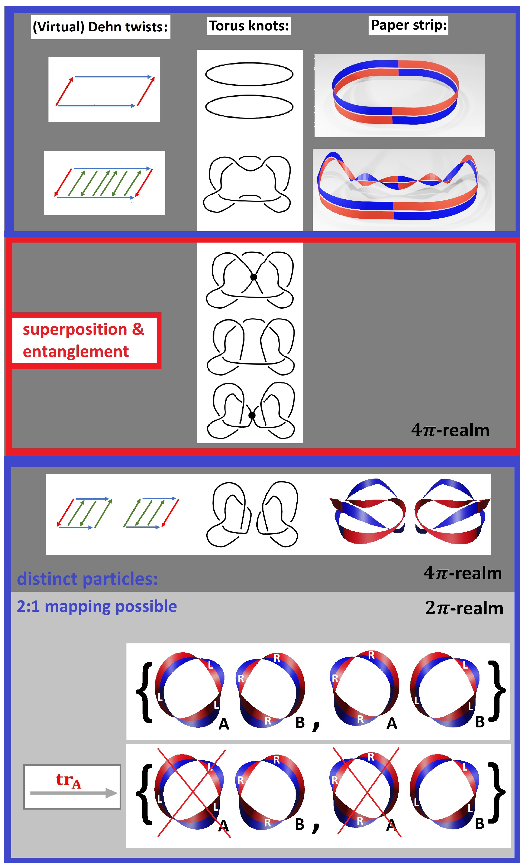
As shown in Figure 15, the combination of Dehn twists with angles ${\mathbf{j}}_1\pi$ and ${\mathbf{j}}_2\pi$ leads in the intermediate state to $|j_1-j_2|\le j_{sum}\le |j_1+j_2|$ Dehn twists, in accordance with the addition rules of angular momentum: In the extreme cases $j_1\pm j_2$, all twists are either added or subtracted from each other, depending on the orientation in which the tori are glued together. Note, that a full $\left(2\pi \right)$-Dehn twist corresponds to the action ℏ.

The importance of Dehn twists for the emission and absorption of vector bosons represented by a tube $T(K_1,K_2)$ connecting two tori (a cobordism) has been discussed in [26,28]. Note the similarity to our approach for a model of particle interaction based on virtual Dehn twists and torus splitting. We leave it for future works to elaborate the relation between these different approaches in greater detail.

Finally, we want to discuss the main topic of this contribution in view of the results achieved: the topological model for the origin of quantum randomness. We arrive at a stroboscopic picture of reality: In the $4\pi$-realm, all transitions between knot structures are smooth and no ‘collapses’ of wave functions exist. No local unitary $SU\left(2\right)$-transformation can induce a change of topology. The simplest example for a unitary operation which induces a change of topology has been given in Section 7.2 as $e^{iHt/\hslash }\in SU\left(4\right)/(SU\left(2\right)\times SU\left(2\right))$. Note, that ladder operators of the type $e_i+i{e}_j$ cannot change the topology of a given quantum state, as discussed in Section 7.3. Crucially, while the transition between a torus, a torus with a virtual (half) Dehn twist and torus splitting to two opposite Klein bottles induced by $e^{iHt/\hslash }$ is smooth and continuous in the $4\pi$-realm, as shown in Figure 7, not all of the intermediate configurations qualify for a 2:1-mapping to the $2\pi$-realm. For this reason, our observation in the $\left(2\pi \right)$-realm leads to quantum randomness: Since the interaction is unobservable in the $\left(2\pi \right)$-realm for topological reasons, we loose track of the relation between initial and final states. In the simple model for quantum randomness introduced in Figure 1, the choice of the “left” and “right” loop must be done in a black box, because this transition is unobservable in the $2\pi$-realm for topological reasons. If the topological model in the $4\pi$-realm is considered an $ontic$ description of of quantum states, randomness hence emerges due to the fact that some features of these states are structurally inaccessible from an $epistemic$ point of view, since human perception is restricted to the realm of observables, that is, the $2\pi$-realm.

In other words, a collapse of the wave function seems to exist only from an epistemic perspective on quantum objects rooted in the $2\pi$-realm, since only a small amount of the knot structures can be mapped here. As interactions are unobservable, Figure 15 suggests the existence of a minimal time step between successive observable states, as the process of changing topology, for example, from the unknot to a pair of complementary $(2j,2)$-torus knots, remains unobservable. In our universe, the explicit value for this minimal time step is the Planck time $t_{Pl}=\sqrt{\left(\hslash G\right)/\left(c^3\right)}\simeq 5.39\times {10}^{-44}s$. While the $existence$ of $t_{Pl}$ follows from our argument, the explicit value cannot be derived.

10. Conclusions and Outlook

We have shown that the simple haptic model for quantum randomness introduced in Section 2 is consistent with the formalism of quantum physics and can be generalized as shown in Figure 15. First, our model has didactical merits due to its striking simplicity, see Figure 1. Second, our key idea to introduce $virtual$ Dehn twists as a new concept to model entanglement as counterpart to a distinction seems to be of interest not only to model quantum randomness, but might also be useful for future research in various perspectives. We think that the simple haptic model for the 2:1 mapping between representations of $SU\left(2\right)\times SU\left(2\right)$ and space-time proposed here is of fundamental importance for the distinction between observable and non-observable physical quantities. In particular, our conjecture is that only those configurations which are obtained by virtual Dehn twists and torus splitting in the $\left(2\pi \right)$-realm qualify for observables. Figure 15 suggests that the ontic viewpopint corresponds to the smooth but unobservable time development in Hilbert space, while the epistemic viewpoint corresponds to the mapping to observables in space-time.

Still, there are open points. For example, our starting point have been distinctions $(A,B)$, their relation to the Lorentz group $SO(3,1)$, its double-cover $SL(2,C)$, and in turn, special relativity. In particular, the $existence$ of a smallest time between two observable states in the $2\pi$-realm follows from our ansatz as shown in Figure 15. As the Planck time $t_{Pl}=\sqrt{\left(\hslash G\right)/\left(c^3\right)}\simeq 5.39\times {10}^{-44}s$ is intimately related to gravity, it is obvious that there must be a relation to knot theory and in turn, entanglement. Recently, much progress has been made in exploring the relation between entanglement and gravity [29,30,31]. Thus, it would be interesting to include gravity in our approach.

However, note that curvature effects and thus effects of general relativity cannot be derived from a simple distinction $(A,B)$, which is a clear limitation of the approach advocated in this contribution. The generalization to curved space time within twistor-theory has been realized by Penrose and Rindler [32,33,34]. For future work, it would be interesting to take into account the importance of the 2:1 mapping between quantum states and observables in such a situation beyond simple distinctions $(A,B)$.

Furthermore, it will be interesting to compare our approach to model entanglement using $virtual$ Dehn twists as counterpart to distinctions $(A,B)$ to recent work in relation to normed divison algebras and variants of the Preon model [8,19,25,26].

While there are many complex and interesting questions waiting for future research, we want to finish this work by once again advocating the striking $simplicity$ of the haptic model for quantum randomness as proposed in Figure 1, which might be of merit also for didactical approaches to quantum and to particle physics: Indeed, not only the stochastic nature of quantum physics, but also the superposition principle and entanglement can be modeled by our approach. Empirical studies will be in need to exploit the effects on learning the basic characteristics of quantum physics.