Identical Limb Dynamics for Unilateral Impairments through Biomechanical Equivalence

Abstract

Dynamic models, such as double pendulums, can generate similar dynamics as human limbs. They are versatile tools for simulating and analyzing the human walking cycle and performance under various conditions. They include multiple links, hinges, and masses that represent physical parameters of a limb or an assistive device. This study develops a mathematical model of dissimilar double pendulums that mimics human walking with unilateral gait impairment and establishes identical dynamics between asymmetric limbs. It introduces new coefficients that create biomechanical equivalence between two sides of an asymmetric gait. The numerical solution demonstrates that dissimilar double pendulums can have symmetric kinematic and kinetic outcomes. Parallel solutions with different physical parameters but similar biomechanical coefficients enable interchangeable designs that could be incorporated into gait rehabilitation treatments or alternative prosthetic and ambulatory assistive devices.

1. Introduction

Human walking is a complex dynamical system. It involves many internal forces and torques that are applied through multiple muscles and joints to create a desired walking trajectory. Developing mathematical models of human walking can play a critical role in discovering new possibilities for healthcare, rehabilitation, and testing many configurations that may not be possible in real experiments [1,2].

Gait is affected by both internal and external factors. The internal factors include parameters such as limb lengths and distribution of mass in the musculoskeletal system. The external factors can also significantly affect the walking performance, such as the slope of the ground, assistive devices, or external stimuli.

Dynamic models are mechanisms that convert kinetic and potential energy to each other in order to create movement. This mechanism is similar to human walking, where the locomotion is the result of moving the center of gravity (CG) of the body while conserving the maximum amount of energy and with minimum displacement of CG in vertical or lateral direction [3]. Dynamic models have been developed in multiple shapes and forms. Their flexible structure could include different point masses, rigid bodies, additional links, dampers, and joints, making them a versatile tool in modeling human limb movements as well as robotic limbs. They typically include two or more connected links or pendulums with point masses and are capable of creating a periodic motion.

There are wide ranges of designs for dynamic models from Passive Dynamic Walkers (PDW) to motorized inverted pendulums. In most cases, the system is first developed and solidified, and then the resultant kinematic and kinetic performance is simulated. Adjustments to the system are only limited to external factors such as external torques, the slope of the ground, or initial conditions. Moreover, the majority of the dynamic models focus on symmetric systems that only imitate healthy gait. Dynamic models have a vast potential to improve our understanding of impaired walking patterns. Furthermore, studying the effects of internal parameters of dynamic models can help answer unknown aspects of disabled gait and improve designs of prosthetics or rehabilitation techniques. Many rehabilitation methods use added weight to one side in order to retrain gait in a symmetrical pattern [4,5]. Finding the optimal distribution of weight in the design of a prosthetic leg can also help create similar dynamics as the healthy leg [6,7].

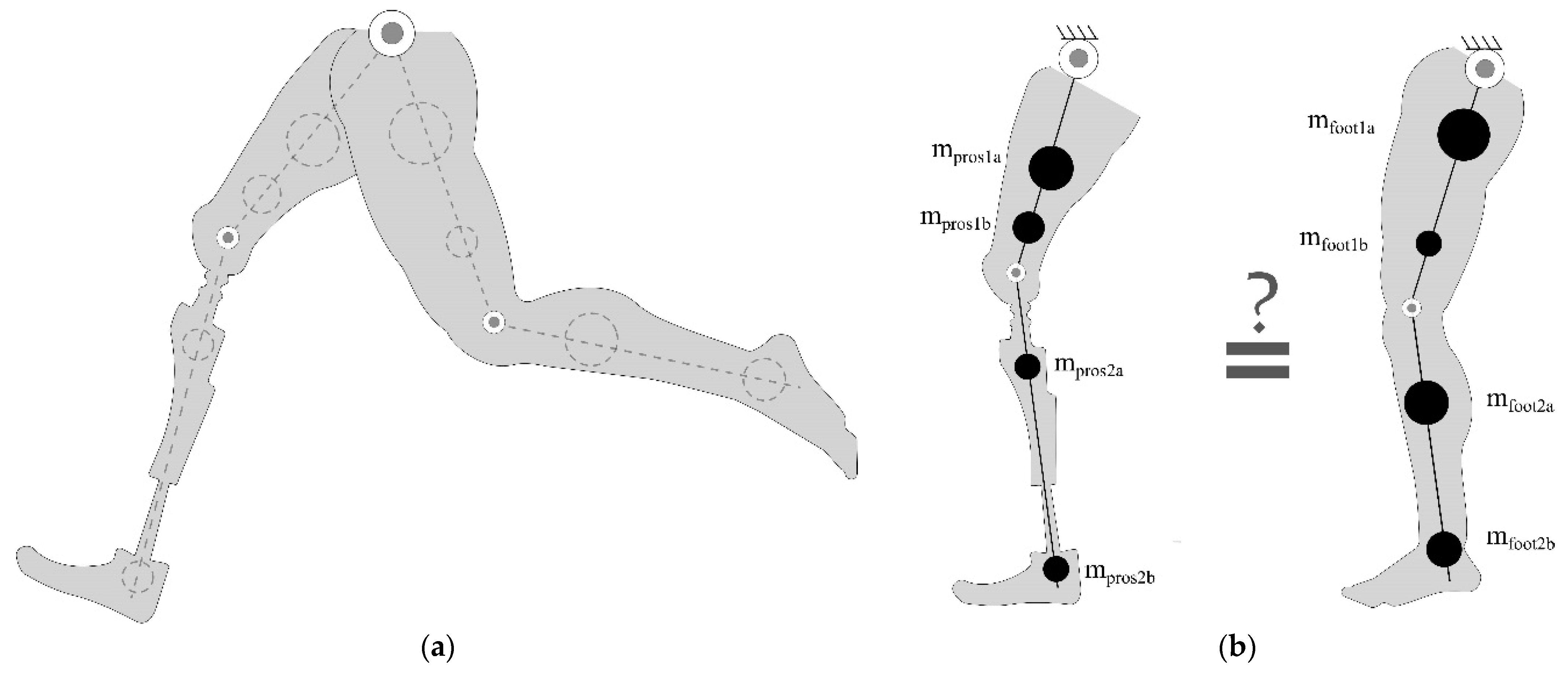
The two legs of an impaired gait can be considered as two dissimilar double pendulum systems (Figure 1), where each system typically has a different trajectory leading to an asymmetric pattern between the steps. In this research, we hypothesize that two double pendulums with different physical parameters can have identical dynamic (motion trajectories and internal forces) outcomes. In other word, inherently asymmetric (dissimilar) double pendulum systems can be kinetically and kinematically matched. This research aims to determine the requirements for perfect symmetry in asymmetric systems.

To test the hypothesis, we first rederive and extend the equations of motion for a double pendulum with various walking events. We use the mathematical equations to introduce a new set of coefficients that determine the biomechanical equivalence between any two systems. The effects of changing physical parameters (such as weight, link length, and center of mass) on these coefficients are studied. Then, we numerically calculate a grouping of systems with similar coefficients and therefore similar kinematics and/or kinetic performance.

2. Background

Reviewing the field of simulating human walking reveals different physical-based methods that have been developed to better understand the walking dynamics, optimize the performance of bipedal robotics, and create mechanisms (such as controllers) that improve walking. Xiang et al. [8] summarized all these methods into five categories, including pendulums, passive dynamic walkers, zero-momentum-point, optimization-based, and control-based. The authors derived the conclusion that the first three methods can be more efficiently used for robotic motions while the two latter can better simulate the complexity of human walking [8].

However, double pendulum systems have shown great potential for simulating human motions [9,10,11,12,13,14]. Simple models with even linear equations of motion can create trajectories similar to human walking and with reasonable accuracy [9]. The presence of gait parameters in the equations improves our understanding of physical movements. Dynamic models also provide a flexible foundation for simulating human walking, where a model outcome can improve through easily upgrading the original equations by adding extra masses to the links or putting external forces to different joints.

While the behavior of a healthy symmetric gait has been studied through symmetric dynamic models, very few of them have been developed to simulate a pathological gait trajectory with asymmetry [15,16,17,18]. One of the limited studies in this area is Asymmetric Passive Dynamic Walkers (APDW) [17,18]. The two-link APDW simulation indicated stable and periodic behavior up to 5% change in the mass and length ratios between the two links [18]. The APDW, with the addition of the knee, was able to walk with a stable pattern over a slope with up to 15% asymmetry between the two links [17]. The follow-up research demonstrated a simulation of lighter prosthetic legs with an asymmetric proportion from the healthy leg that produced a symmetric walking trajectory [6]. Comparing the simulation result with human experiments with asymmetric gait (adding extra weight to one leg) indicated a similar pattern and Ground Reaction Forces (GRF) between the model and human data [19].

However, achieving a symmetric trajectory within an asymmetric dynamic model is not possible with every configuration. Handžić et al. [20] demonstrated that having only one mass on each link of a double pendulum system couples the moments of inertia. Therefore, any change in the system parameters would mean a change in the motion trajectory or force reactions since not enough parameters (masses, moments, or moments of inertia) exist to compensate for the change. However, adding a second point mass to each link creates an underdetermined system that would allow for a change in parameters without a change in kinematics. The authors derived kinematically matched coefficients (KMC) that determine for kinematically matching systems.

Dissimilar systems yielding similar motion can have a hugely beneficial effect in our understanding of pathologic limb movements and consequently, the rehabilitation of the asymmetric gait. Prosthetic limb users, crutch walkers, and stroke survivors all have asymmetrical movements and can benefit from the alternative gait pattern that produces symmetric motions. In this research, we analyze the motion of double pendulum systems under different conditional constraints and study both the kinetic and kinematic outcomes.

This research develops on the KMC concept and extends it to include human-like events such as ground strike and knee-lock. It also investigates the kinetic outcomes of dissimilar systems and introduces new sets of coefficients for a comprehensive analysis. The goal of the current research is to answer the research question of whether “kinematic and kinetic symmetry can be achieved within an inherently asymmetric system?”

3. Mathematical Modeling

In this section, we rederive kinematic and kinetic equations of a double pendulum system. The double pendulum has four masses (two per link) with hinge joints at the top (hip) and between the two links (knee). Figure 2 shows the double pendulum parameters, including mass locations, links lengths, and the angle of each link at a given time. Two local polar coordinate systems were attached at the hinge of each link.

3.1. Kinematic Measurments

In order to derive the equations of motion using Lagrangian mechanics, total kinetic, and potential energies of the system are calculated. ${\theta }_1$ and ${\theta }_2$ are the angle of the first link with vertical line and the angle of the second link with the first link, respectively. ${\dot{\theta }}_1$ and ${\dot{\theta }}_2$ are the angular velocities with respect to time. ${\ddot{\theta }}_1$ and ${\ddot{\theta }}_2$ are the angular accelerations. Step-by-step details of calculating the equations of motion are depicted in Appendix A.

Calculating Lagrange’s equations for the variables of the system and reorganizing the order of parameters will result in two equations of motion as Equations (1) and (2):

$$\begin{array}{l}[m_{1a}{l}_{1a}^2+m_{1b}{\left(l_{1a}+l_{1b}\right)}^2+m_{2a}(l_1^2+l_{2a}^2+2l_1{l}_{2a}\cos {\theta }_2)+m_{2b}(l_1^2\\ +{\left(l_{2a}+l_{2b}\right)}^2+2l_1\left(l_{2a}+l_{2b}\right)\cos {\theta }_2)]{\ddot{\theta }}_1\\ +[m_{2a}(l_{2a}^2+l_1{l}_{2a}\cos {\theta }_2)+m_{2b}({(l_{2a}+l_{2b})}^2+l_1(l_{2a}\\ +l_{2b})\cos {\theta }_2]{\ddot{\theta }}_2\\ -2[m_{2a}{l}_1{l}_{2a}\sin {\theta }_2+m_{2b}{l}_1(l_{2a}+l_{2b})\sin {\theta }_2]{\dot{\theta }}_1{\dot{\theta }}_2\\ -[m_{2a}{l}_1{l}_{2a}\sin {\theta }_2+m_{2b}{l}_1(l_{2a}+l_{2b})\sin {\theta }_2]{\dot{\theta }}_2^2\\ +[m_{1a}{l}_{1a}+m_{1b}(l_{1a}+l_{1b})+m_{2a}{l}_1+m_{2b}{l}_1]g\sin {\theta }_1\\ +[m_{2a}{l}_{2a}+m_{2b}(l_{2a}+l_{2b}\left)\right]g\sin ({\theta }_1+{\theta }_2)=0\end{array}$$

(1)

$$\begin{array}{l}\left[m_{2a}{l}_{2a}\left(l_{2a}+l_1\cos {\theta }_2\right)+m_{2b}\left(l_{2a}+l_{2b}\right)\left(l_{2a}+l_{2b}+l_1\cos {\theta }_2\right)\right]{\ddot{\theta }}_1\\ +[m_{2a}{l}_{2a}^2+m_{2b}{\left(l_{2a}+l_{2b}\right)}^2]{\ddot{\theta }}_2\\ +\left[m_{2a}{l}_1{l}_{2a}\sin {\theta }_2+m_{2b}{l}_1\left(l_{2a}+l_{2b}\right)\sin {\theta }_2\right]{\dot{\theta }}_1^2\\ +\left[m_{2a}{l}_{2a}+m_{2b}\left(l_{2a}+l_{2b}\right)\right]g\sin \left({\theta }_1+{\theta }_2\right)=0\end{array}$$

(2)

Nine ($m_{1a}, l_{1a},m_{1b},l_{1b},m_{2a},l_{2a},m_{2b},l_{2b},l_1$) out of the ten physical parameters with the exception of $l_2$ are used in the derivation of Equations (1) and (2). However, when the equations are reorganized, only a limited number of combinations of these parameters show up. Here, we define five new coefficients for replacing the physical parameters in Equations (1) and (2) using the KMCs developed in [20,21]. These combinations are shown in Equations (3)–(7). $a, b, d, e$, and $f$ represent new combinations of parameters.

$$a=m_{2a}{l}_{2a}^2+m_{2b}{\left(l_{2a}+l_{2b}\right)}^2$$

(3)

$$b=\left[m_{2a}{l}_{2a}+m_{2b}\left(l_{2a}+l_{2b}\right)\right]\times l_1$$

(4)

$$d=m_{2a}{l}_{2a}+m_{2b}\left(l_{2a}+l_{2b}\right)$$

(5)

$$e=m_{1a}{l}_{1a}+m_{1b}\left(l_{1a}+l_{1b}\right)+\left(m_{2a}+m_{2b}\right)l_1$$

(6)

$$f=m_{1a}{l}_{1a}^2+m_{1b}{\left(l_{1a}+l_{1b}\right)}^2+\left(m_{2a}+m_{2b}\right)l_1^2$$

(7)

The equations of motions can be rewritten as:

$$\begin{array}{l}\left[\begin{array}{cc}f+a+2b\cos {\theta }_2& a+b\\ a+b\cos {\theta }_2& a\end{array}\right]\left[\begin{array}{c}{\ddot{\theta }}_1\\ {\ddot{\theta }}_2\end{array}\right]-\left[\begin{array}{cc}0& b\sin {\theta }_2\\ b\sin {\theta }_2& 0\end{array}\right]\left[\begin{array}{c}{\dot{\theta }}_1{}^2\\ {\dot{\theta }}_2{}^2\end{array}\right]\\ -\left[\begin{array}{cc}b\sin {\theta }_2& b\sin {\theta }_2\\ 0& 0\end{array}\right]\left[\begin{array}{c}{\dot{\theta }}_1{\dot{\theta }}_2\\ {\dot{\theta }}_2{\dot{\theta }}_1\end{array}\right]+\left[\begin{array}{c}g(e\sin {\theta }_1+d\sin \left({\theta }_1+{\theta }_2\right)\\ gd\sin \left({\theta }_1+{\theta }_2\right)\end{array}\right]\\ =0\end{array}$$

(8)

Equation (8) represents the kinematic motion of a double pendulum with two point-masses on each link at any given time. Further details of this analysis can be found in [20,21]. To represent the straight leg system with the knee hinge locked, ${\theta }_2$ is set to zero which results in a single pendulum system with four masses. This single pendulum system can partially be derived from Equation (8), but also needs to consider the Lagrange equations of motion. The first Lagrange equation described above is determined by taking the derivative with respect to ${\theta }_1$ and the second includes the derivation with respect to ${\theta }_2$. ${\theta }_1$ continues to represent the hip angle; however, ${\theta }_2$ represents a locked knee with a constant value. For the single pendulum using the above double pendulum model, ${\theta }_2$ and the corresponding derivatives need to be set to zero, which means the system only has one degree of freedom. Thus, there is no second variable to use in a second Lagrange equation of motion. Even if the derivative was taken with respect to ${\theta }_2$, all of the terms would go to zero because ${\theta }_2$ does not appear (i.e., it is set to zero). Thus, the second row in Equation (8) does not have meaning nor a mathematical basis in the single pendulum system. Therefore, the first row in Equation (8) is the only equation of motion for a single pendulum with four mass system. Equation (9) can be derived by either setting ${\theta }_2=0$ in the first row of Equation (8) or by deriving from the Lagrange equation:

$$\left(f+a+2b\right){\ddot{\theta }}_1+g\left(e+d\right)\sin {\theta }_1=0$$

(9)

Equations (8) and (9) indicate the kinematics for a double and single pendulum with four masses and no external force, respectively. They demonstrate that only the defined biomechanical coefficients need to be matched between two systems to have the same motion trajectories and not the full set of physical parameters. In the following section, we derive mathematical equations for knee-lock and ground-strike during walking. We model these events using the collision principle. We also introduce new kinetically matched coefficients to describe the internal forces of hip and knee joints.

3.2. Collisions

Collision or impact is the sudden change of motion between two or more bodies that happens due to the objects colliding and alters internal forces within them. Two types of collisions can be defined in dynamic models that mimic human walking [22]. The first one is the knee-lock event and happens when the bent leg straightens out. In terms of dynamic models, during the knee-lock event, the double pendulum switches to a single pendulum by locking the hinge between the two links and preventing the second link from moving toward the opposite side. The second event is the contact with outside surfaces such as hitting the ground during heel strike or impact with an obstacle.

Collisions can be defined from perfectly elastic to perfectly inelastic depending on the loss of kinetic energy and the coefficient of restitution (E) [23]. A collision with no loss of kinetic energy and E = 1 is a perfectly elastic collision, and a collision with maximum kinetic energy loss and E = 0 is perfectly inelastic. No matter of the collision type, angular momentum during a collision is always conserved if no external force or impulse is applied. During impact (collision with external force), on the other hand, an external impulse is applied to the system. The change in angular momentum before and after an impact will be equal to the angular impulse applied during the time of contact with the external object.

3.2.1. Knee-Lock

As a result of a knee-lock event, equations of motion for the system switches from Equations (8) and (9). However, angles and angular velocities change due to this collision. The new values can be calculated based on the before collision condition. In a leg with two links, ${\theta }_2$ is always bigger or equal to zero; meaning the knee cannot bend backward. Therefore, at ${\theta }_2=0$, the middle hinge (knee) is locked, and the double pendulum is turned into a single pendulum. The dynamic model right before and after the knee collision is depicted in Figure 3.

The before and after conditions are shown with + and − superscripts, and since no external force is involved, conservation of angular momentum is applicable:

$$\mathsf{\Delta }P={\displaystyle \sum }{P}^{+}-{\displaystyle \sum }{P}^{-}=0$$

(10)

$${\displaystyle \sum }_{i=0}^n{\overrightarrow{r_i}}^{-}\times m_i{\overrightarrow{V_i}}^{-}={\displaystyle \sum }_{i=0}^n{\overrightarrow{r_i}}^{+}\times m_i{\overrightarrow{V_i}}^{+}$$

(11)

The total angular momentums before and after knee-lock are shown in Equations (12) and (13).

$$\begin{array}{l}{\displaystyle \sum }{P}^{-}=[m_{1a}{l}_{1a}^2+m_{1b}{\left(l_{1a}+l_{1b}\right)}^2+\left(m_{2a}+m_{2b}\right)l_1^2+m_{2a}{l}_{2a}^2+m_{2b}{\left(l_{2a}+l_{2b}\right)}^2\\ +2l_1\cos {\theta }_2^{-}(m_{2a}{l}_{2a}+m_{2b}\left(l_{2a}+l_{2b}\right))]{\dot{\theta }}_1^{-}\\ +[m_{2a}{l}_{2a}^2+m_{2b}{\left(l_{2a}+l_{2b}\right)}^2+l_1\cos {\theta }_2^{-}(m_{2a}{l}_{2a}+m_{2b}(l_{2a}\\ +l_{2b}))]{\dot{\theta }}_2^{-}\end{array}$$

(12)

$${\displaystyle \sum }{P}^{+}=[m_{1a}{l}_{1a}^2+m_{1b}{\left(l_{1a}+l_{1b}\right)}^2+m_{2a}{\left(l_1+l_{2a}\right)}^2+m_{2b}{\left(l_1+l_{2a}+l_{2b}\right)}^2]{\dot{\theta }}_1^{+}$$

(13)

Applying the conservation of angular momentum will result in a transfer matrix $Q$, as shown in Equation (14). After the knee-lock, the second link only moves due to the movement of the first link. Therefore, the second row of the transfer matrix is zero in Equation (15). After reorganizing the equations of angular momentum, all the parameters in the first row of the transfer matrix can be replaced using the same kinematic coefficients ($a,b,d,e,$ and $f$):

$${\dot{\theta }}^{+}=Q\times {\dot{\theta }}^{-}$$

(14)

$$Q=\left[\begin{array}{cc}{q}_{11}& q_{12}\\ 0& 0\end{array}\right]=\left[\begin{array}{cc}\frac{f+a+2b\cos {\theta }_2^{-}}{f+a+2b}& \frac{a+b\cos {\theta }_2^{-}}{f+a+2b}\\ 0& 0\end{array}\right]$$

(15)

Thus, both equations of motion for the double pendulum and single pendulum as well as the knee-lock collision were modeled and rewritten by the same coefficients ($a,b,d,e$, and $f$). The following section studies the double pendulum movement under collision with external surfaces.

3.2.2. External Surfaces

The lower limbs repeatedly interact with the ground during walking. Each step ends with the corresponding foot hitting the ground. Ground collisions are almost always modeled as a perfectly inelastic collision, meaning that the maximum loss of kinetic energy happens during contact, and the two collided bodies (ground and the foot) stay attached without any slipping. However, in reality, more scenarios such as partially elastic heel-strike, tripping over an object, or slipping could happen. Modeling similar events in the double pendulum system can create an improved dynamic model that simulates similar behavior to human walking. Moreover, modeling collision with objects in the workspace is beneficial for robotic limb motions.

Here, the case of the double pendulum hitting different external surfaces on the trajectory path is considered. Similar to PDWs and other dynamic models [22], it is assumed that the contact happens during knee-lock, but whether the system stays in that position will depend on the condition of the collision.

Figure 4 shows the different predicted outcomes that could happen during contact with external objects. Regardless of the collision type, we assume the obstacle, or the wall, is located at a distance $\lambda$ and the condition for the contact to happen will be:

$$\left(l_1+l_2\right)\sin {\theta }_1>\lambda$$

(16)

Therefore, for the collision to happen at the same time for two dissimilar double pendulums, the total length of the systems ($l_1+l_2$) needs to be the same. An additional new kinematic coefficient ($h$) replaces the physical parameters ($l_1 \mathrm{and} l_2$) and defines this condition:

$$h=l_1+l_2$$

(17)

In a perfectly inelastic collision (Figure 4a), the maximum amount of kinetic energy is lost. It is also assumed that the wall has infinite mass. The angular velocity immediately after the collision is zero. The pendulum is completely stopped by the wall, and all the kinetic energy of the system is lost. It is interesting to note that even in a perfectly inelastic collision, the angular momentum of the system is conserved. The assumption is that the external surface (the wall) has infinite mass, the velocity of the colliding system after collision becomes zero as shown in Equations (18)–(20).

$${\displaystyle \sum }{P}^{-}={\displaystyle \sum }{P}^{+}$$

(18)

$${\displaystyle \sum }_{All pendulum masses}{r}_i\times m_i{v}_i+M_{wall}\times 0=\left(\sum m_i+M_{wall}\right)V^{+}$$

(19)

$$V^{+}=\underset{M_{wall}\to \infty }{\lim }\frac{{{\displaystyle \sum }}_{All pendulum masses}{r}_i\times m_i{v}_i}{\sum m_i+M_{wall}}=0$$

(20)

However, the double pendulum is not at the equilibrium position during the collision and will start to move due to gravity. The potential energy will start to convert to kinetic energy. This collision does not add any new coefficient.

Calculation for perfectly elastic collision and tripping event (Figure 4b,c) are described in detail in Appendix B. It is important to note that all the physical parameters in the collision events (perfectly inelastic, perfectly elastic, and tripping) as well as equations of motion were replaced by only 6 coefficients, namely $a,b,d,e, f$, and $h$. Therefore, kinematic symmetry between two dissimilar legs can be achieved through symmetry of these biomechanical coefficients.

Modeling slipping (Figure 4d) on the surface introduces the stick-slip mechanism to the system. Calculating the velocity of the pendulum over the surface will depend on the static and kinetic friction coefficients between the wall and the pendulum at the contact point. This paper does not model this type of collision because this situation requires a lot of information and therefore assumptions about the material of the surface such as the shape of the second link foot, the static and kinetic friction coefficients between the two objects, and so on.

3.3. Kinetic Measurements

Figure 5 shows the internal forces at the two hinges of the double pendulum. The forces are indicated in a 2-dimensional plane and in the direction of the local coordinate of each link. Newton’s second law is used to calculate the forces at any given time during the motion of the double pendulum.

For the first hinge ($H_1$):

$$\begin{array}{ll}{F}_{H1r}=& -\left[m_{1a}+m_{1b}+m_{2a}+m_{2b}\right]g\cos {\theta }_1-[m_{2a}{l}_{2a}\\ & +m_{2a}\left(l_{2a}+l_{2b}\right)]\sin {\theta }_2{\ddot{\theta }}_2\end{array}$$

(21)

$$\begin{array}{ll}{F}_{H1\theta }=& -\left[m_{1a}+m_{1b}+m_{2a}+m_{2b}\right]g\sin {\theta }_1\\ & +\left[m_{1a}{l}_{1a}+m_{1a}\left(l_{1a}+l_{1b}\right)+\left(m_{2a}+m_{2b}\right)l_1\right]{\ddot{\theta }}_1+[m_{2a}{l}_{2a}\\ & +m_{2a}\left(l_{2a}+l_{2b}\right)]\cos {\theta }_2{\ddot{\theta }}_2\end{array}$$

(22)

For the second hinge ($H_2$):

$$F_{H2r}=-\left(m_{2a}+m_{2b}\right)g\cos \left({\theta }_1+{\theta }_2\right)$$

(23)

$$F_{H2\theta }=\left(m_{2a}+m_{2b}\right)g\sin \left({\theta }_1+{\theta }_2\right)+\left[m_{2a}{l}_{2a}+m_{2a}\left(l_{2a}+l_{2b}\right)\right]{\ddot{\theta }}_2$$

(24)

Replacing the parameters of the system with the coefficients Equations (3)–(7) and introducing two new coefficients for kinetic forces, $k$ and $s$:

$$k=m_{1a}+m_{1b}+m_{2a}+m_{2b}$$

(25)

$$s=m_{2a}+m_{2b}$$

(26)

The forces are rewritten as:

$$F_{H1r}=-kg\cos {\theta }_2-d\sin {\theta }_2{\ddot{\theta }}_2$$

(27)

$$F_{H1\theta }=kg\sin {\theta }_2+e{\ddot{\theta }}_1+d\cos {\theta }_2{\ddot{\theta }}_2$$

(28)

$$F_{H2r}=-sg\cos \left({\theta }_1+{\theta }_2\right)$$

(29)

$$F_{H2\theta }=sg\sin \left({\theta }_1+{\theta }_2\right)+d{\ddot{\theta }}_2$$

(30)

Six coefficients for the kinematic models ($a,b,d,e, f$, and $h$) define the equations of motion, knee-lock collision, and multiple types of collision with external surfaces. Achieving kinetic symmetry in addition to kinematic symmetry, introduces two more kinetic coefficients ($k$ and $s$).

The combined eight equations (Equations (3)–(7), (25), and (26)) for the biomechanical coefficients ($a,b,d,e, f,h,k$, and $s$) include all ten physical parameters of the double pendulum ($m_{1a}, m_{1b}, l_{1a}, l_{1b}, l_1, m_{2a}, m_{2b}, l_{2a}, l_{2b}, l_2$). If all eight coefficients between two different double pendulums are identical, they are kinematically and kinetically symmetric. Since there are ten variables within the coefficients, the system of equations is underdetermined ($n=8$ equations and $m=10$ variables with $n<m$). The underdetermined system creates the possibility of systems with different physical parameters but similar coefficients. However, the coefficient equations are quadratic and nonlinear. There are analytical methods for solving nonlinear pendulum system with collision [24] but not all the solutions are acceptable. Negative or complex solutions are not physically acceptable values. Positive values outside of anthropometric data will not be humanly realizable models. Therefore, it is important to look for answers that are physically and humanly realizable. Two masses per link are the minimum number needed to allow an underdetermined system and can allow for sufficient modeling of a human limb. Three or more masses per link could be used if needed for modeling but does not provide additional benefits beyond the two for synchronizing the motion.

4. Results

We analyze and numerically solve the undetermined system of coefficients for human realizable configurations. The analysis includes the case of achieving only kinematic symmetry ($n=6$) and both kinematic and kinetic symmetry ($n=8$). The case of only kinetic symmetry between two systems is not possible since internal forces depend on the same acceleration and configuration at each moment.

4.1. Kinematic Symmetry

Two kinematically matched double pendulum systems will move in unison, given they start at the same initial conditions. However, the internal forces within the joints will not necessarily be the same. Six out of the eight coefficients’ equations ($a,b,f,d,e,h$) describe only kinematic symmetry. Looking closely at coefficients $b$ and $d$ indicates that $l_1$ is constant. Furthermore, coefficient $h$ reveals that $l_2$ will stay constant as well. With $l_1$ and $l_2$ constant, a reduced underdetermined system of four equations ($a,f,d,e$) and eight variables ($m_{1a},m_{1b},l_{1a},l_{1b},m_{2a},l_{2a},m_{2b},l_{2b}$) remains.

$a,f,d,e$ equations can numerically be solved for kinematic symmetry. These coefficients are also physically meaningful and represent biomechanical properties. They are moments and moments of inertia for the second link and the entire pendulum. We use a numerical approach to solve for a set of humanly realizable data. The sample is chosen for an average anthropometric dataset from [25]. It is important to note that current anthropometric datasets only report total mass of each link and do not report mass distribution data. Therefore, we assumed an arbitrary distribution of masses on each link.

Table 1. Humanly realizable sample system for the numerical solution.

	${\mathit{m}}_{1\mathit{a}}$	${\mathit{l}}_{1\mathit{a}}$	${\mathit{m}}_{1\mathit{b}}$	${\mathit{l}}_{1\mathit{b}}$	${\mathit{l}}_1$	${\mathit{m}}_{2\mathit{a}}$	${\mathit{l}}_{2\mathit{a}}$	${\mathit{m}}_{2\mathit{b}}$	${\mathit{l}}_{2\mathit{b}}$	${\mathit{l}}_2$
Sys H 1	4.0	0.2	3.5	0.2	0.6	2	0.1	1.5	0.2	0.5

¹ All masses are in kilogram (kg) and lengths are in meter (m).

shows the data for the sample system. The numerical method can solve for all possible combinations of physical parameters that result in the same coefficients as Sys H. We also apply physical restrictions such as $l_{1a}+l_{1b}\le l_1$ and $l_{2a}+l_{2b}\le l_2$. The range for each variable is set between zero and twice in value, and the precision for length values is set to 0.05.

The numerical method tested $~{10}^5$ combinations and resulted in 365 parallel solutions (about ~0.3% of tested combinations) that match the human realizable criteria. Figure 6 shows four examples of these systems compared to Sys H. The first example indicates the lightest possible double pendulum design that creates the same kinematic outcome as Sys H. The second parallel system has the heaviest total mass. The third and fourth examples demonstrate the lowest and highest ratio of the first link total mass to the second link. All these dissimilar double pendulum models create the same trajectory of motion, angular positions, velocities, and acceleration for both links for all time assuming they start at the same position. Each system in this grouping is different from others in physical parameters, but all of them have the same kinematic coefficient values, meaning all the kinematic equations will result in the same output. The system of coefficients represents a lot of potential for optimizing the design without sacrificing the desired outcomes. This benefit gets more important when designing rehabilitation devices for disabled people. Creating assistive devices such as prosthetic legs that are mechanically capable of creating a symmetric gait pattern and are lighter in weight could potentially improve the walking experience and efficiency for amputees, crutch users, and stroke survivors.

Figure 7 demonstrates an application of dissimilar double pendulums using the systems in Figure 6. If an amputee has the same anthropometric data as Sys H on their healthy leg (Figure 7a), designs of a prosthetic leg that can have similar kinematic outcomes could benefit from the 365 derived systems with similar kinematic coefficients.

Figure 7b shows the lightest prosthetic leg design with a 10% decrease in total mass. Figure 7c demonstrates a design that minimizes the ratio of total mass between the two links by 25.2%. Similar kinematics between a healthy leg and a prosthetic leg can assist with the improvement of symmetric gait patterns where both sides are able to walk with similar step times and step lengths.

4.2. Full Symmetry

While systems with kinematic symmetry have similar trajectories, the forces generated in the hip or knee joint might not be the same. To achieve kinetic symmetry along with kinematic symmetry, all eight of the coefficients ($a,b,d,e, f,h,k$, and $s$) between two dissimilar systems should be the same. Section 3.1 numerically solves the first six kinematic equations. The final two kinetic coefficients, $k$ and $s$, represent the total mass of the whole system and the second link, respectively. This section generates a full symmetry analysis.

Numerically solving for the additional $k$ and $s$ equations results in 60 parallel solutions (less than one percent (~0.06%) of all the $~{10}^5$ tested combinations). These systems match all eight coefficients of Sys H.

Figure 8 indicates the variations in mass values and mass locations between these parallel solutions. All these systems result in the same kinematic and kinetic outcomes while having different physical parameters. The similar biomechanical coefficients between these parallel solutions would mean that these systems have the same total mass, moment, and moment of inertia in the whole system and the second link (Equations (3)–(7), (25) and (26)). For instance, a maximum mass value in $m_{2a}$ (Figure 8a) is accompanied by a minimum mass value in $m_{2b}$ of the same system.

Among the 60 solution, $l_{2b}$ did not change much and only had three different values. Therefore, the boxplot of this parameter in Figure 8b does not have data points for a complete Whisker plot. The numerical method solves the underdetermined system of coefficients for a subset of possible solutions. Increasing the precision and range of the variables can return more answers for the datasets.

4.3. Simulations

As a proof of concept, this section simulates the results of kinematic and kinetic outcomes. The simulations demonstrate the outcomes of the anthropometric data of a healthy leg, and two of sample systems derived based on the matching coefficients with similar biomechanics, one with only kinematic symmetry and one with full symmetry.

Table 2. Humanly realizable sample systems for the numerical solution.

	${\mathit{m}}_{1\mathit{a}}$	${\mathit{l}}_{1\mathit{a}}$	${\mathit{m}}_{1\mathit{b}}$	${\mathit{l}}_{1\mathit{b}}$	${\mathit{l}}_1$	${\mathit{m}}_{2\mathit{a}}$	${\mathit{l}}_{2\mathit{a}}$	${\mathit{m}}_{2\mathit{b}}$	${\mathit{l}}_{2\mathit{b}}$	${\mathit{l}}_2$
Kinematic 1	3.56	3.50	0.30	0.10	0.6	1.78	1.28	0.15	0.15	0.5
Full 2	6.50	1.00	0.25	0.29	0.6	3.00	0.50	0.15	0.28	0.5

¹ Sample system with only kinematic symmetry. ² Sample system with full (kinetic and kinematic) symmetry.

shows these samples.

The simulation results compare the angle, angular velocity, angular acceleration, and the reaction forces at both joints. The modeling considers the different cases of plastic or elastic collision and impact with external surfaces. The goal of this section is to show that the new coefficients introduced in this research can accurately predict similarity in kinematic and kinetic outcomes of dissimilar double pendulums.

Figure 9 introduces the algorithm logic. The programming was written in MATLAB R2019a. The double pendulum starts with an initial condition as an input. At every increment of time, the angular positions, velocities, and accelerations of the two links are calculated. The system can be locked at the hinge so as to not allow the second link to move toward the opposite side. Therefore, if ${\theta }_2$ becomes zero, the knee is locked, and the double pendulum switches to a single pendulum. During the single pendulum mode and before reaching the external surface ($(l_1+l_2)\sin {\theta }_1<\lambda$), a pseudo-double pendulum tracks the angular position and angular velocity of the unlocked second link at every time step. The moment ${\theta }_2$ in the pseudo-double pendulum turns positive, the real system is unlocked and will switch back to the double pendulum mode.

When the system reaches the external surface ($(l_1+l_2)\sin {\theta }_1=\lambda$), three different types of collisions (described in Section 3.2.2) can happen. Based on the condition of the knee joint and elasticity of the collision, the results of a perfectly elastic collision, perfectly inelastic, or an impulse impact were simulated.

Figure 10 shows the results for two sample systems of Table 2 along with the original data, Sys H, from Tabel 1. As expected, the system with only kinematic symmetry had the same trajectory (Figure 10a,b) as the original anthropometric data (Sys H); however, the joints’ forces were different. The system with full symmetry matched the trajectory as well as the forces at the joints (Figure 10a–d) of Sys H.

5. Discussion

Dynamic models such as double pendulums offer a simple yet flexible approach for understanding the biomechanics of impaired walking. They closely simulate human walking patterns. Each leg can be modeled as a double pendulum with two links (thigh and calf) connected with a hinge (knee). Dissimilar double pendulums can mimic asymmetric limbs where the physical characteristic of each side is different from the other. This theoretical modeling helps us understand the influence of physical parameters of legs on kinematic and kinetic performance. This outcome can help develop assistive devices and rehabilitation techniques capable of generating identical dynamics in inherently asymmetric gaits.

This research redefines the kinematic and kinetic equations describing double pendulums, including equations of motion, collision events, and internal forces at the joints. A set of new biomechanical coefficients is defined. They replace all physical parameters of the system in the mathematical equations. We indicated that not all parameters individually affect the outcome of the double pendulum; rather, combinations of them (biomechanical coefficients) collectively influence the kinematic and kinetic performance. This discovery helps us choose different systems that can create the same desired motion or force reaction. This flexibility can significantly help in creating symmetric walking in a gait with unilateral impairment. For instance, a prosthetic leg can be designed to have the same step time and step length as the healthy leg.

The double pendulum model in this research has ten different physical parameters. We introduce eight biomechanical coefficients (6 for kinematic equations and 2 for kinetic equations). We replace all the physical parameters in the equations with these coefficients. Therefore, they shape an underdetermined system with more physical parameters in the system than biomechanical coefficients required for symmetry. Using anthropometric data, we then numerically solve the underdetermined system for physically and humanly meaningful answers.

We found 365 solutions (about ~0.3% of $~{10}^5$ tested combinations) for kinematic symmetry and 60 solutions (~0.06% of all the tested combinations) for full symmetry. Simulation of the sample systems for the anthropometric data confirmed the accuracy of the coefficients in achieving kinematic and kinetic symmetry.

There are some limitations in this research that future studies can improve. This paper only investigates the theoretical motion of the impaired gait. A follow-up study is needed to experimentally validate this model in clinical application. The physical simulation of ground impact does not study slipping. Future studies can expand the simulation to include analytical solutions, additional masses on each link, a foot model at the tip, external forces and torques, and friction.

Achieving identical limb dynamics can enhance the quality of life for patients with unilateral impairments. Future clinical studies can validate and incorporate the double pendulum model for various rehabilitation applications. For instance, a physical therapist can utilize this theoretical model to modify the weight training in stroke therapy. Another example is to use the pendulum measurements for customizing the design of prosthetic legs for optimal performance.

6. Conclusions

This research introduces a new idea to redefine the modeling of dynamic systems. We introduce a set of biomechanical coefficients that act as a connection between the physical parameters of the system and multipliers defining the dynamic equations. In a system with fewer coefficients than parameters, a range of flexibility in the design can create asymmetric systems that have biomechanical equivalence. These innovative coefficients can potentially help improve our understanding of asymmetric gait and optimize the techniques and devices that promote symmetry.

References

- Santos, C.C.; Barbosa, T.M.; Bartolomeu, R.F.; Garrido, N.D.; Costa, M.J. Inter-Limb Symmetry at Simultaneous and Alternated Arms Flexion by the Elbow during Water Fitness Sessions. Symmetry 2020, 12, 1776. [Google Scholar] [CrossRef]
- Smajla, D.; Knezevic, O.M.; Mirkov, D.M.; Šarabon, N. Interlimb Asymmetries and Ipsilateral Associations of Plantar Flexors and Knee Extensors Rate-of-Force Development Scaling Factor. Symmetry 2020, 12, 1522. [Google Scholar] [CrossRef]
- Tucker, C.A.; Ramirez, J.; Krebs, D.E.; Riley, P.O. Center of gravity dynamic stability in normal and vestibulopathic gait. Gait Posture 1998, 8, 117–123. [Google Scholar] [CrossRef]
- Muratagic, H.; Ramakrishnan, T.; Reed, K.B. Combined effects of leg length discrepancy and the addition of distal mass on gait asymmetry. Gait Posture 2017, 58, 487–492. [Google Scholar] [CrossRef]
- DeBolt, L.S.; McCubbin, J.A. The Effects of Home-Based Resistance Exercise on Balance, Power, and Mobility in Adults with Multiple Sclerosis. Arch. Phys. Med. Rehabil. 2004, 85, 290–297. [Google Scholar] [CrossRef]
- Sushko, J.; Honeycutt, C.; Reed, K.B. Prosthesis design based on an asymmetric passive dynamic walker. In Proceedings of the 2012 4th IEEE RAS & EMBS International Conference on Biomedical Robotics and Biomechatronics (BioRob), Rome, Italy, 24–27 June 2012; pp. 1116–1121. [Google Scholar]
- Hoffman, M.D.; Sheldahl, L.M.; Buley, K.J.; Sandford, P.R. Physiological comparison of walking among bilateral above-knee amputee and able-bodied subjects, and a model to account for the differences in metabolic cost. Arch. Phys. Med. Rehabil. 1997, 78, 385–392. [Google Scholar] [CrossRef]
- Xiang, Y.; Arora, J.S.; Abdel-Malek, K. Physics-based modeling and simulation of human walking: A review of optimization-based and other approaches. Struct. Multidiscip. Optim. 2010, 42, 1–23. [Google Scholar] [CrossRef]
- Goswami, A.; Thuilot, B.; Espiau, B. Compass-Like Biped Robot Part I: Stability and Bifurcation of Passive Gaits. Doctoral Dissertation, INRIA, Le Chesnay-Rocquencourt, France, 1996. [Google Scholar]
- Petró, B.; Kiss, B.; Kiss, R.M. Analyzing human balance recovery action using calculated torques of a double pendulum model. Mater. Today Proc. 2019, 12, 431–439. [Google Scholar] [CrossRef]
- Aguilar-Sierra, H.; Yu, W.; Salazar, S.; Lopez, R. Design and control of hybrid actuation lower limb exoskeleton. Adv. Mech. Eng. 2015, 7, 1–13. [Google Scholar] [CrossRef]
- El Zahraa Wehbi, F.; Huo, W.; Amirat, Y.; El Rafei, M.; Khalil, M.; Mohammed, S. Active impedance control of a knee-joint orthosis during swing phase. In Proceedings of the 2017 International Conference on Rehabilitation Robotics (ICORR), London, UK, 17–20 July 2017; pp. 435–440. [Google Scholar]
- Singh, S.; Mukherjee, S.; Sanghi, S. Study of a self-impacting double pendulum. J. Sound Vib. 2008, 318, 1180–1196. [Google Scholar] [CrossRef]
- Bazargan-Lari, Y.; Gholipour, A.; Eghtesad, M.; Nouri, M.; Sayadkooh, A. Dynamics and control of locomotion of one leg walking as self-impact double pendulum. In Proceedings of the 2nd International Conference on Control, Instrumentation and Automation, Shiraz, Iran, 27–29 December 2011; pp. 201–206. [Google Scholar]
- Gregg, R.D.; Degani, A.; Dhahe, Y.; Lynch, K.M. The Basic Mechanics of Bipedal Walking Lead to Asymmetric Behavior. In Proceedings of the IEEE International Conference on Rehabilitation Robotics, Zurich, Switzerland, 29 June–1 July 2011; pp. 816–821. [Google Scholar]
- Gregg, R.; Dhaher, Y.; Degani, A.; Lynch, K. On the Mechanics of Functional Asymmetry in Bipedal Walking. IEEE Trans. Biomed. Eng. 2012, 59, 1310–1318. [Google Scholar] [CrossRef] [PubMed]
- Honeycutt, C.; Sushko, J.; Reed, K.B. Asymmetric passive dynamic walker. In Proceedings of the 2011 IEEE International Conference on Rehabilitation Robotics, Zurich, Switzerland, 29 June–1 July 2011; 2011; pp. 1–6. [Google Scholar]
- Rasouli, F.; Naraghi, M.; Safa, A.T. Asymmetric gait analysis based on passive dynamic walking theory. In Proceedings of the International Conference on Robotics and Mechatronics (ICROM), Tehran, Iran, 26–28 October 2016; pp. 361–366. [Google Scholar]
- Handžíc, I.; Reed, K.B. Validation of a Passive Dynamic Walker Model for Human Gait Analysis. In Proceedings of the Annual International Conference of the IEEE Engineering in Medicine and Biology Society, EMBS, Osaka, Japan, 3–7 July 2013; pp. 6945–6948. [Google Scholar]
- Handžíc, I.; Muratagic, H.; Reed, K.B. Passive kinematic synchronization of dissimilar and uncoupled rotating systems. Nonlinear Dyn. Syst. Theory 2015, 15, 383–399. [Google Scholar]
- Muratagic, H. Passive Symmetry in Dynamic Systems and Walking. Master’s Thesis, University of South Florida, Tampa, FL, USA, 2015. [Google Scholar]
- Chen, V.F.H. Passive Dynamic Walking with Knees: A Point Foot Model, Massachusetts Institute of Technology. Doctoral Dissertation, Massachusetts Institute of Technology, Cambridge, MA, USA, 2005. [Google Scholar]
- Alrasheed, S. Principles of Mechanics: Fundamental University Physics; Springer Nature: Cham, Switzerland, 2019. [Google Scholar]
- Guo, X.; Zhang, G.; Tian, R. Periodic solution of a non-smooth double pendulum with unilateral rigid constrain. Symmetry 2019, 11, 886. [Google Scholar] [CrossRef] [Green Version]
- Huston, R.L. Principles of Biomechanics; CRC Press: Boca Raton, FL, USA, 2008. [Google Scholar]
Figure 1.
Dynamic model of an asymmetric human gait with double pendulums: (a) Modeling of an impaired gait with two different double pendulum systems; (b) different mass distributions on each leg represented by for the prosthetic side and for the healthy side with . The hypothesis in this study evaluates whether the two different legs can be made to move symmetrically.
Figure 2.
Double pendulum system with four masses. Each link includes two masses at different locations. The top and bottom links replicate shank and thigh motion, respectively. The top and middle hinges represent hip and knee joints, respectively.
Figure 3.
Double pendulum before and after the knee-lock event. The before and after angles are shown with + and − superscripts.
Figure 4.
Double pendulum colliding with different external surfaces: (a) Perfectly inelastic collision with ground; (b) perfectly elastic collision with ground; (c) tripping over an object; (d) slipping over the contact surface.
Figure 5.
Internal forces of the system at each hinge during movement.
Figure 6.
Kinematically parallel system to Sys H with lightest total mass, heaviest total mass, lowest links’ mass ratios, and highest links’ mass ratios.
Figure 7.
Prosthetic leg designs based on the anthropometric data of a healthy leg: (a) Anthropometric data for a healthy leg; (b) a dynamic model of a prosthetic design with symmetric kinematics and lightest weight; (c) a dynamic model of another prosthetic design with symmetric kinematics and the lowest ratio of mass between the links.
Figure 8.
Variation in physical parameters between systems with full symmetry. Red lines indicate the median. The square specifies the lower and upper quartiles. Whiskers show the minimum and maximum values in each parameter. (a) Whisker plot of mass values, and in full symmetric pendulum systems; (b) Whisker plot of each mass locations, and in full symmetric pendulum systems.
Figure 9.
Algorithm flowchart for simulation of a double pendulum system with knee-lock and different collisions with external surfaces. Yellow diamonds indicate the conditional statements and make decisions depending on the answer to the questions. Red circles are instance changes in the state of the system under a sudden collision. Blue rectangles are the processors for calculating the state of the system (angles, angular velocities, angular accelerations).
Figure 10.
Kinematic and kinetic simulations of systems with different physical parameters but similar kinematic and kinetic coefficients. Sys H, Sys Kin, and Sys Full indicate the result for the anthropometric data, a sample of systems (365 solutions) with only kinematic symmetry, and a sample of systems (60 solutions) with full symmetry, respectively. (a) Angular displacement; (b) angular acceleration; (c) internal forces at hip joint; (d) internal forces at the knee joint.