Abstract
This paper describes the stability and Hopf bifurcation analysis of the Brusselator system with delayed feedback control in the single domain of a reaction–diffusion cell. The Galerkin analytical technique is used to present a system equation composed of ordinary differential equations. The condition able to determine the Hopf bifurcation point is found. Full maps of the Hopf bifurcation regions for the interacting chemical species are shown and discussed, indicating that the time delay, feedback control, and diffusion parameters can play a significant and important role in the stability dynamics of the two concentration reactants in the system. As a result, these parameters can be changed to destabilize the model. The results show that the Hopf bifurcation points for chemical control increase as the feedback parameters increase, whereas the Hopf bifurcation points decrease when the diffusion parameters increase. Bifurcation diagrams with examples of periodic oscillation and phase-plane maps are provided to confirm all the outcomes calculated in the model. The benefits and accuracy of this work show that there is excellent agreement between the analytical results and numerical simulation scheme for all the figures and examples that are illustrated.
1. Introduction
Over the last fifty years, many nonlinear chemical applications with diffusion reactions have been explained and studied analytically and numerically via the use of partial differential equations (PDEs), for instance, the Belousov–Zhabotinsky (BZ) reaction [1], the Brusselator model [2], the pellet model [3], the reversible Selkov [4], and the Gray and Scott cubic autocatalytic systems [5,6]. Furthermore, the nonlinear (and quasilinear) diffusive models are of great interest for a large and increasing number of practical applications in many applied mathematics fields, for instance see [7,8] and [9]. These models discuss various chemical oscillatory phenomena in our daily lives using a continuous-flow stirred-tank reactor (CSTR) [10]. The CSTR drives a perfect result in both theoretical and experimental examinations of oscillatory chemical models [2,6,11,12].
One of the most important chemical reaction models was discovered in 1968 [13] and is called the Brusselator model. The nonlinear diffusive Brusselator system consists of two species of BZ model. This model has been discussed by many researchers. For example, ref. [2] examined the analytical results of the Brusselator model in both 1D and 2D domains. Galerkin’s technique was applied to determine the ordinary differential equations (ODEs) drawn from the PDEs in the model. As a consequence, perfect solutions were explored to show the stability of the Hopf bifurcation analysis. Many researchers have referred to references concerning the Brusselator model with reaction–diffusion, see [14,15,16,17,18,19] and the references therein.
The existence of feedback with a delay time term in PDE models is extremely important as it can strongly affect the stability of the model. It can also change the results of the Hopf bifurcation analysis [12,20,21]. The authors of [22] considered delayed feedback control for the Brusselator system with reaction–diffusion. They determined that the delayed feedback control caused the formation of extreme events [22,23], where there was a large parameter value, and that the delayed feedback control caused instability. The authors illustrated numerical simulation examples to prove their theoretical outcomes.
A dynamic analytical solution to a nonlinear PDE system can be obtained in many ways. However, some of the models are difficult to examine. Here, I provide an analytical method that is a reliable technique used widely to drive nonlinear PDEs. The Galerkin analytical technique [24] has been used to provide an analytical result that presents a comparison between the numerical simulation PDE model and the theoretical analysis of the ODE system. This method provides a comparison with the analytical solution to demonstrate the accuracy of analytical results. Some examples that use this method include the Selkov–Schnakenberg reaction–diffusion system [25], the BZ model [1], Nicholson’s blowflies system [26], neural network systems [27], logistic equations with delays [12,28,29,30], the Gray and Scott cubic autocatalytic system [6], viral infection models [11], and the food-limited equation [31]. In general, all the researchers that have applied this method reported an extremely agreeable comparison between the theoretical ODE results and the numerical scheme of the PDE model.
The Brusselator system with delayed feedback control in 1D cells was studied in this work. Research studies are lacking on the effect of a delayed feedback control term in the diffusive Brusselator model. Furthermore, there is not enough detail explaining the effects of delayed feedback control on the overall stability and Hopf bifurcation analysis. Hence, additional research is needed on the effect of these parameters on the PDE model. Thus, our primary objective was to derive the theoretical ODE results by using the Galerkin method. This work offers an explanation of how to find the Hopf bifurcation points. In addition, to construct full map diagrams of the Hopf bifurcation points and the stability analysis (stable and unstable regions), I use examples of periods in the limit cycle maps and the 2D phase-plane maps.
This paper is arranged as follows. Section 2 details the nonlinear PDE model with delayed feedback control under the Dirichlet boundary condition. In Section 3, Galerkin’s method is described, which helps to find a system for the delay ODE equations. Section 4 presents the methodology and theoretical framework to present how the Hopf bifurcation maps devolve. Section 5 develops the stability of the concentration cells in the Hopf bifurcation maps and provides the bifurcation diagrams and limited cycle of stable and unstable results. This is in addition to the 2D phase-plane graphs for both the theoretical results of the ODEs and the numerical simulation of the PDE solutions.
2. Mathematical Formulations Model
The diffusive Brusselator model with delayed feedback control is a nonlinear system of PDEs as follows:
where X and Y refer to the activator and inhibitor, respectively, in the dimensionless concentrations of two reactants (interacting chemical species) at time t; A and B indicate two control parameter concentrations during the reaction process; D denotes the diffusion coefficient of two reactants in the system; H refers to the delayed feedback parameter, which is the strength of the feedback control; and describes the time delay in the feedback term. Note that the approximation that uses the delay value is useful in relation to the limit where the strength of the delay has both small and large values. In this term, the chemical feedback concentrations are small enough for their development to be explored via a single term of delay. This system is open, and the result has a symmetrical pattern at the center of the domain . Furthermore, and are the positive initial concentrations when the time ranges between . Note that are used in all numerical simulations exemplified in this work. A Crank–Nicolson finite-difference scheme [30,32] is used to obtain the numerical solutions of the PDE model (1). Furthermore, I consider the Runge–Kutta method [3,33] to show the numerical simulation results of the ODE semi-analytical system (3). The numerical examples used for spatial and temporal discretization are and . Note that these values are appropriate to obtain numerical convergence (this implicit scheme is unconditionally stable).
3. The Galerkin Technique Methodology
Galerkin’s technique [24] applies orthogonality to the base function collections to convert PDE into ODE systems. This technique is important and useful. It considers a temporal–spatial separation and explores a spatial form of profile density [3,6]. Galerkin’s technique is an analytical method that employs the orthogonality of the rudimentary roles set to find the ODE system from the PDE model. This method has been widely applied to solve nonlinear PDEs in many models and applications [26,27,29,30]. The following equations are trial functions:
where and . The trial equation function is built as , and variable denotes the middle of the profile concentrations . The trial equation expansions (2) meet the boundary conditions in the PDE system in (1). The free variables of the values in the model are then explored by computing the values of the PDEs with delay. Next, the PDEs are weighted by two trial function expansions: and . The resulting system of four ODE equations is presented as follows:
Note that the equations in (2) have been abbreviated at the two-term expansion point. This is so that the two-term outcome provides sufficient reliability in terms of accuracy without an extreme swell in expression. It also provides good results compared with the numerical scheme of the PDE system. In addition, the system of the one-term equations can be shown via letting in the first two equations in the ODE system (3).
4. Theoretical Framework for the Existence of Hopf Bifurcation
This section analytically describes the methodologies that explore the existence of Hopf bifurcation points. There is a curve that divides the region stability into stable and unstable areas; this curve consists of Hopf bifurcation points. Hopf bifurcation denotes the periodic limit cycle oscillation occurrence in the neighborhood of the steady state that can move the solutions from stable to unstable outcomes. As a result, the conjugated pair of eigenvalues passes into the imaginary axis. For more details, see [20,21,34]. The points of the Hopf bifurcation are determined by discovering the evolution of the Taylor series built for the steady-state parameters. This can be examined as:
Therefore, the expressions and as in (4) are replaced in the ODE system (3). Then, the steady-state parameters are linearized. Next, the Jacobian matrix of eigenvalues considers a small system perturbation that demonstrates the typical growth value k. This is achieved by placing in the single equation of the characteristic. This equation can be separated into two different equations: real () and imaginary (). Therefore, the next condition equation can solve the Hopf bifurcation point:
5. Stability and Hopf Bifurcation Analysis
5.1. Hopf Bifurcation Areas
This section provides the Hopf bifurcation maps for the stable and unstable regions presented as semi-analytical maps of ODEs (3), comparing the analytical outcomes to the numerical simulation of the PDE results. Furthermore, I studied the effects of all free parameters in the system () on the regions of the Hopf bifurcation during the reaction process. At the end of this section, I provide a special numerical example to demonstrate the accuracy and advantage of the analytical method over the numerical simulation PDE results. Note that the Hopf bifurcation point can be determined by solving the condition Equation (3); these points compose a curve that divides the stability region into stable and unstable regions.
Figure 1a,b show maps of the two areas of the Hopf bifurcation in versus concentrations of input reagents A and B, respectively. The positive values that were used are , , and in Figure 1a and in Figure 1b. In Figure 1a, there are two areas provided: the upper part is the stable zone and the lower part is the unstable zone. It shows that as delay parameter increases, the rate of the Hopf bifurcation points for control A reduce slowly. However, in Figure 1b, two different regions are plotted but oppositely to Figure 1a. In contrast, this figure shows that the Hopf bifurcation points for chemical input control B increase steadily as delay parameter increases. Therefore, we find good agreement amongst the analytical outcomes of the two terms with the PDE numerical simulation with no more than a error for all of the selected parameters in the domain up to .
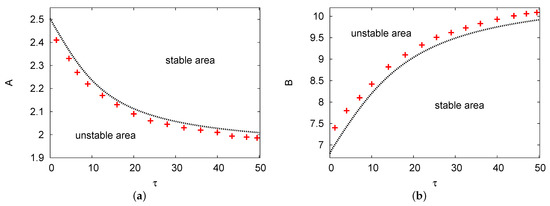
Figure 1.
(color online) (a,b) The Hopf bifurcation curves in the and maps. The line of red crosses refers to the results of the partial differential equation (PDE) numerical simulation and the black dots are the results of the two terms in the semi-analytical system. The positive values that were used are , , and in (a) and in (b).
Figure 2a,b illustrate the Hopf bifurcation curves in the and planes. The parameters used were , , and for Figure 2a; and , , and for Figure 2b. In both cases, the numerical PDE simulation (line of red crosses) and the analytical results of the two terms (solid black line) are displayed. As in the previous figure, there are two areas in each figure: unstable and stable areas. In Figure 2a, as feedback parameter H increases, the values of the Hopf bifurcation points of the control parameter concentration B increase considerably. However, in Figure 2b, the Hopf bifurcation points for control B decrease as diffusion parameter D increases. Both figures show a good agreement between the analytical outcomes of the two terms compared with the simulation results of the PDE system in all chosen parameters related to the domain.
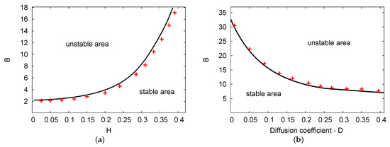
Figure 2.
(color online) (a,b) The Hopf bifurcation lines of the and planes. The analytical simulation results for the two terms (black solid line) and the numerical simulation of the PDEs (line of red crosses) were obtained. The parameters used were , , and for (a); and , , and for (b).
Figure 3a,b displays the Hopf bifurcation points for concentrations of input reagent A against chemical control B, with different examples of feedback parameter H and diffusion value D, respectively. The numerical values are and in Figure 3a, and and in Figure 3b. The analytical outcomes of the two-term equations are used in both figures. There are two areas shown in both cases: the stable and unstable areas. In both figures, as the control parameter concentration A increases, the value of B increases dramatically and the solutions move up from left to right. In Figure 3a, four examples of feedback parameter H are selected: , and . In this figure, at any fixed point selected for chemical control parameter concentration A, the value of control parameter B increases as feedback control parameter H increases. However, for Figure 3b, five examples of diffusion coefficient parameter D were chosen: , and . From these examples, it can be observed that at any fixed point of A, the parameter of control B reduces as the diffusion coefficient value D increases. Note that the resulting behavior displayed in this figure is similar to the case where , see [24]. Therefore, the values of feedback parameter H and diffusion term D can significantly impact the control parameter concentrations during the reaction process.
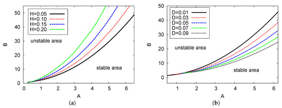
Figure 3.
(color online) (a,b) The Hopf bifurcation maps in the diagrams versus examples of feedback parameter H and the diffusion parameter D, respectively. The two-term semi-analytical simulation is plotted. The parameter values applied here were and for (a); and and for (b).
Figure 4a,b demonstrate the Hopf bifurcation regions for the maps and the plane, respectively. Two-term analytical results were obtained in both cases. The parameter values used are , , and in Figure 4a; for Figure 4b, the values used are , , and . In Figure 4a, the two areas considered as the Hopf bifurcation points of the diffusion coefficient D increase linearly as feedback parameter H increases. In addition, Figure 4b shows that the diffusion parameters grow slowly in relation to the small range of the D value versus the increase in delay parameter . Therefore, the diffusion coefficient values have more of an impact on feedback control parameter H than delay variable .
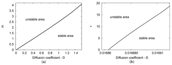
Figure 4.
(a,b) The Hopf bifurcation areas for diffusion coefficient value D against the parameters of feedback control H and delay value , respectively. The semi-analytical outcomes of the two-term results are plotted. The parameter values used were , , and for (a); in (b), , , and .
Figure 5a compares the Hopf bifurcation map for the diagrams with the two cases of feedback control parameter H: , showing no feedback control term (red dotted curve), and feedback control parameter (black solid line). The Hopf bifurcation point decreases (at fixed chemical control B) moving from the non-feedback control term compared with the feedback control rate case . Figure 5b depicts the control parameter concentration of B versus the frequency of limit cycle for the two cases of and . The frequency of the periodic result in Figure 5b increases as the value of B increases. For both values of feedback control, the difference between the values showing the frequency of the limit cycle, , is extremely small with an error rate of less than 1% across all the values of control parameter concentration B.
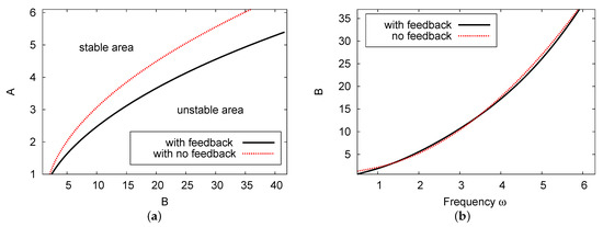
Figure 5.
(color online) (a) The Hopf bifurcation map in the plane and (b) the frequency of the periodic results against B. Here, we can see the results for two cases: , where there is no feedback control term; and the curve. The other parameter values are and .
Comparisons were performed for the special parameters of , , , and . In this case, the points of the Hopf bifurcation exist at for the one-term outcome, whereas in the analysis of the two-term result. The numerical simulation result of the PDE system is . All these results predict the incidence of the Hopf bifurcation analysis shown in this example as reliable and in agreement. The error rate between the numerical simulation and the theoretical results is less than 1%.
5.2. Bifurcation Diagrams, Periodic Oscillation, and Phase-Plane Map
In this part, I chose control parameter concentration B as the bifurcation parameter. The steady-state results where (no delay case) are provided. I constructed bifurcation diagrams and studied the impact of the other free parameters in the diagrams and limit cycle maps. Furthermore, the maps of the phase plane in the 2D domain are also plotted. The maps of the bifurcation diagrams were examined at the center of the domain and the limit cycles are plotted over a long time period for time t.
Figure 6 displays the steady state of the two chemical concentrations of reaction products X and Y versus control parameter B, where and . It reveals the analytical outcomes for the two- and one-term systems and the numerical simulation of the presented PDE scheme. There are unique pattern steady-state results for the concentrations of activator X and inhibitor Y. Figure 6a illustrates that as control parameter B increases, the dimensionless concentration activator X decreases significantly before approaching a minimum point at . The curve of reactant concentration inhibitor Y increases gradually as control parameter B increases in Figure 6b. When the concentration B value is large, the reactant concentration of activator X has a small value (near zero), while reactant concentration Y increases exponentially. There is very good agreement between the numerical model of the PDE simulations and the analytical results of the ODE system, with no more than a 1% error rate in the domain of the concentration of the reactant.
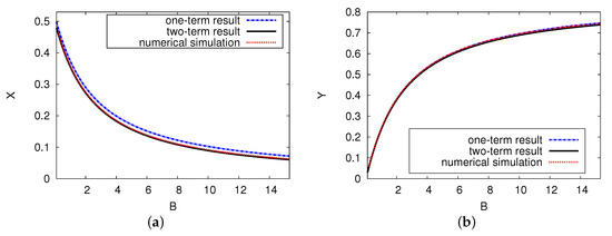
Figure 6.
(color online) The steady-state concentration of the interacting chemical species of X and Y versus control B. The analytical results for one and two terms are shown as a black solid and a blue dashed curve, respectively. The red dotted points refer to the numerical simulation of the PDE model. The parameters used were and .
Figure 7 depicts the bifurcation diagram of the dimensionless chemical concentrations of reactants X and Y versus control parameter concentration B. In this illustration, the PDE numerical simulation and the analytical outcomes of both one and two terms are presented and are shown as being closely related. The positive parameters applied in these figures are , , and . This example shows the importance of the existence of a time delay in the model with a feedback control term, which can make a positive steady state unstable and thus induce instability. In both cases, the periodic solutions have a supercritical Hopf bifurcation from which the reactant concentrations of X and Y are derived. Thus, the Hopf bifurcation points for the analytical outcomes for both one and two terms are and , respectively. The Hopf bifurcation of the numerical simulation result of the PDE is . It can be seen that as the value of the chemical control parameter B increases, so does the maximum amplitude of the oscillations. The minimum amplitude is still low, and therefore, the predictions concerning the analytical outcomes of the two terms agree with the numerical simulation of the PDE predictions.
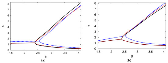
Figure 7.
(color online) (a,b) The bifurcation map of reactant concentrations X and Y versus control parameter concentration B. The analytical results for one and two terms are indicated by black solid and blue dashed curves, respectively. The PDE numerical simulation (dotted red curve) is also shown. The parameters used were , , , and .
Figure 8 illustrates the bifurcation plane of the chemical concentrations of two chemical species X and Y versus control parameter concentration B with three examples of the delayed feedback control parameter H: (blue dashed), (black solid), and (red dotted). The analysis of the two-term outcomes is provided for each instance with positive parameters of and . The supercritical Hopf bifurcation points in the reactant concentrations X and Y were found to be at , and 2.99 for the cases of delayed feedback parameter H = 0.05, 0.10, and 0.15, respectively. It is clear that increasing the delayed feedback parameter stabilizes the system and causes control parameter concentration B to move back when there is an increase in the strength of the delay (feedback parameter H). The results shown in this figure confirm the outcomes in Figure 2a. The point of the Hopf bifurcation related to the control chemical B moves forward with the increase in diffusion coefficient D through the concentrations of the two reactants X and Y.
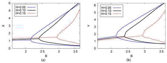
Figure 8.
(color online) (a,b) The bifurcation diagram of chemical concentrations X and Y against control concentration B for three different cases of feedback control parameter H: H = 0.05, 0.10, and 0.15. The analytical results of the two terms are plotted. The values of the parameters were , , and .
Figure 9a,b both show the reactant concentrations of the two interacting chemical species X and Y against time in the center of the domain. The parameters used were , , , , and (Figure 7). The analytical outcomes of one and two terms with the numerical simulation of the PDEs are shown. The results show a steady state at and with an increase in time after a few periodic oscillations. The agreement between the two-term analytical and numerical simulation PDE results is excellent, with an error rate less than 2% in the steady state over a long time t.
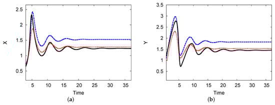
Figure 9.
(a,b) The reactant concentrations of the two interacting chemical species X and Y against time. The one-term analysis is shown as a blue dashed line; the black solid line indicates the analytical results of the two-term analysis. The numerical simulation of the PDE system (red dotted line) is plotted. The parameters used were , , , , and (color available online).
Figure 10 shows a limited cycle curve for chemical concentrations X and Y versus time t. The parameters in these figures are the same as in Figure 10, where . This point forms the unstable region in Figure 7. The periodic solution is shown over a long time. The length of the numerical simulation of the period of the limit cycle for the reactant concentrations is and the amplitudes of oscillation are and for the chemical concentrations of the two reaction products X and Y, respectively. The analytical two-term results in the limit cycle period and amplitude were approached according to the PDE simulation scheme. The period is and the amplitudes are and for the concentrations of the two reactants of X and Y, respectively, with less than a 1.5% error rate between them.
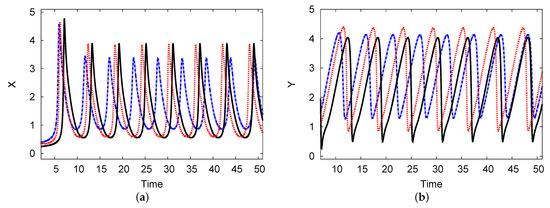
Figure 10.
(color online) (a,b) The limit cycle maps for the reactant concentrations X and Y over time. The analytical results for one and two terms are shown as black solid and blue dashed curves, respectively, and the PDE numerical scheme (dotted red curve) is also presented. The parameters used were , , , , and .
Figure 11a shows the phase plane of the 2D maps for chemical concentration X against Y (activator and inhibitor), where , , , , and . The scheme of the numerical PDE simulation and one- and two-term analytical output was determined. The numerical simulation of the PDE outcomes approaches the analytical two-term results. Figure 11b presents the phase plane of the 2D maps showing the analytical results of the two terms with four different examples of chemical control concentration B: B = 3, 3.5, 4, and 4.5. It is evident that as control concentration rate B increases, the limit cycle increases regularly. This result indicates that there is no doubling or chaos in the limit cycle in this system [26].
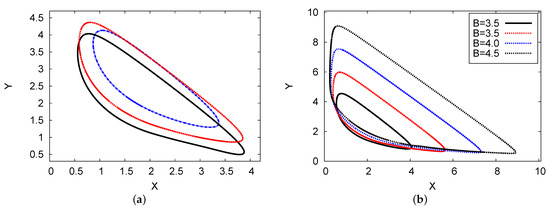
Figure 11.
(color online) (a) The phase planes in a 2D map for the concentration of reactant X against Y. The analytical results of the two-term (red dotted line) and one-term (blue dashed line) results are plotted, where the black solid line represents the numerical simulation scheme of the PDE results, with , , , and . (b) 2D phase-plane maps for the two-term analytical outcomes with four different examples of B: (solid black), (dotted red), (dotted blue), and B = (dotted black).
Figure 12a shows the phase space of the two chemical concentrations of the reaction products X against Y for three various examples of the feedback parameters of H (in the left plane) and diffusion coefficient D (in the right map). The analysis of the two-term outcome is given for both cases. The parameter values used were , , and with for Figure 12a, and in Figure 12b. The three examples of D are 0.05, 0.03, and 0.01; H = 0.15 and 0.10; and . In both figures, the limit cycle (oscillation amplitude) decreases as diffusion coefficient D and feedback parameter H increase. In Figure 12a, when , the solution will be stable; in Figure 12b, the result can move from unstable to stable outcomes after point .
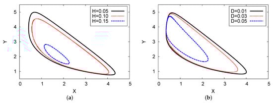
Figure 12.
(color online) Limit cycle map for the two-term analytical results: , , and for three different examples of H and D, with for (a), and for (b).
6. Conclusions
In this study, I constructed a lower-order analytical system of delayed feedback control for the Brusselator model in the 1D domain. A system of delay ODEs was derived from Galerkin’s technique. Hopf bifurcation analysis was determined both theoretically and numerically. The Hopf bifurcation points consisted of a curve that divided each graph into two different areas of stability (stable and unstable). Hopf bifurcation diagrams for the two concentrations of the respective control parameters were plotted. In addition, the effects of the time delay, feedback control, and diffusion parameters were studied in detail. These parameters have a strong impact on the instability and are significant for the two concentration reactants (interacting chemical species) in the system. The solutions in this work were developed as shown by the various examples of stable and unstable limit cycles and the phase plane in the 2D maps. The comparison of the analytical two-term outcome against the PDE scheme for the numerical simulation results facilitated the use of the semi-analytical technique. It is worth using this method as it is a very effective and precise analytical method in relation to a PDE system. In future work, I plan to apply this method to another chemical reaction cell with two different delays in the feedback control.
Author Contributions
The author carried out the proofs of the main results and approved the final manuscript. The author has read and agreed to the published version of the manuscript.
Funding
This research received no external funding.
Institutional Review Board Statement
Not applicable.
Informed Consent Statement
Not applicable.
Data Availability Statement
Not applicable.
Acknowledgments
The author wishes to thank the anonymous referees and editor for their useful comments.
Conflicts of Interest
The author declares that there are no conflict of interest regarding the publication of this paper.
References
- Alfifi, H.Y.; Marchant, T.R.; Nelson, M.I. Non-smooth feedback control for Belousov-Zhabotinskii reaction-diffusion equations: Semi-analytical solutions. J. Math. Chem. 2016, 57, 157–178. [Google Scholar] [CrossRef]
- Alfifi, H.Y. Semi-analytical solutions for the Brusselator reaction-diffusion model. ANZIM J. 2017, 59, 167–182. [Google Scholar] [CrossRef]
- Marchant, T.R.; Nelson, M.I. Semi-analytical solution for one-and two-dimensional pellet problems. Proc. R. Soc. Lond. 2004, A460, 2381–2394. [Google Scholar] [CrossRef]
- Al Noufaey, K.S.; Marchant, T.R. Semi-analytical solutions for the reversible Selkov model with feedback delay. Appl. Math. Comput. 2014, 232, 49–59. [Google Scholar] [CrossRef]
- Alharthi, M.R.; Marchant, T.R.; Nelson, M.I. Mixed quadratic-cubic autocatalytic reaction-diffusion equations: Semi-analytical solutions. Appl. Math. Model. 2014, 38, 5160–5173. [Google Scholar] [CrossRef]
- Marchant, T.R. Cubic autocatalytic reaction diffusion equations: Semi-analytical solutions. Proc. R. Soc. Lond. 2002, A458, 873–888. [Google Scholar] [CrossRef]
- Merz, W.; Rybka, P. Strong solutions to the Richards equation in the unsaturated zone. J. Math. Anal. Appl. 2010, 371, 741–749. [Google Scholar] [CrossRef]
- Berardi, M.; Difonzo, F. Strong solutions for Richards’ equation with Cauchy conditions and constant pressure gradient. Environ. Fluid Mech. 2020, 20, 165–174. [Google Scholar] [CrossRef]
- Liu, B.; Marchant, T.R. The microwave heating of two-dimensional slabs with small Arrhenius absorptivity. IMA J. Appl. Math. 1999, 62, 137–166. [Google Scholar] [CrossRef]
- Gray, P.; Griffiths, J.F.; Scott, K. Branched-chain reactions in open systems: Theory of the oscillatory ignition limit for the hydrogen+ oxygen reaction in a continuous-flow stirred-tank reactor. Proc. R. Soc. Lond. 1984, A394, 243–258. [Google Scholar]
- Alfifi, H.Y. Semi-analytical solutions for the delayed and diffusive viral infection model with logistic growth. J. Nonlinear Sci. Appl. 2019, 12, 589–601. [Google Scholar] [CrossRef]
- Alfifi, H.Y. Semi analytical solutions for the Diffusive Logistic Equation with Mixed Instantaneous and Delayed Density Dependencel. Adv. Differ. Equ. 2020, 162, 1–15. [Google Scholar]
- Prigogine, I.; Lefever, R. Symmetry Breaking Instabilities in Dissipative Systems. II. J. Chem. Phys. 1968, 48, 1665–1700. [Google Scholar] [CrossRef]
- Adomian, G. The diffusion-Brusselator equation. Comput. Math. Appl. 1995, 29, 1–3. [Google Scholar] [CrossRef]
- Ang, W. The two-dimensional reaction-diffusion Brusselator system: A dual-reciprocity boundary element solution. Eng. Anal. Bound. Elem. 2003, 27, 897–903. [Google Scholar] [CrossRef]
- Mittal, R.; Jiwari, R. Numerical study of two-dimensional reaction-diffusion Brusselator system. Appl. Math. Comput. 2011, 217, 5404–5415. [Google Scholar] [CrossRef]
- Kumar, Y.K.S.; Yildirim, A. A mathematical modeling arising in the chemical systems and its approximate numerical solution. Asia Pac. J. Chem. Eng. 2012, 7, 835–840. [Google Scholar] [CrossRef]
- Twizell, E.; Gumel, A.; Cao, Q. A second-order scheme for the Brusselator reaction-diffusion system. J. Math. Chem. 1999, 26, 297–316. [Google Scholar] [CrossRef]
- Wazwaz, A. The decomposition method applied to systems of partial differential equations and to the reaction-diffusion Brusselator model. Appl. Math. Comput. 2000, 110, 251–264. [Google Scholar] [CrossRef]
- Erneux, T. Applied Delay Differential Equations; Springer: New York, NY, USA, 2009. [Google Scholar]
- Hale, J. Theory of Functional Differential Equations; Springer: New York, NY, USA, 1977. [Google Scholar]
- Tlidi, M.; Gandica, Y.; Sonnino, G.; Averlant, E.; Panajotov, K. Self-Replicating Spots in the Brusselator Model and Extreme Events in the One-Dimensional Case with Delay. Entropy 2016, 18, 64. [Google Scholar] [CrossRef]
- Akhmediev, N.; Kibler, B.; Baronio, F.; Belić, M.; Zhong, W.P.; Zhang, Y.; Chang, W.; Soto-Crespo, J.M.; Vouzas, P.; Grelu, P.; et al. Roadmap on optical rogue waves and extreme events. J. Opt. 2016, 18, 063001. [Google Scholar] [CrossRef]
- Fletcher, C.A. Computational Galerkin Methods; Springer: New York, NY, USA, 1984. [Google Scholar]
- Al Noufaey, K. Stability analysis for Selkov-Schnakenberg reaction-diffusion system. Open Math. 2021, 19, 46–62. [Google Scholar] [CrossRef]
- Alfifi, H.Y.; Marchant, T.R.; Nelson, M.I. Semi-analytical solutions for the 1- and 2-D diffusive Nicholson’s blowflies equation. IMA J. Appl. Math. 2014, 79, 175–199. [Google Scholar] [CrossRef]
- Alfifi, H.Y. The stability and Hopf bifurcation analysis for the delay diffusive neural networks model. AIP Conf. Proc. 2020, 2184, 1–8. [Google Scholar]
- Alfifi, H.Y. Stability and Hopf bifurcation analysis for the diffusive delay logistic population model with spatially heterogeneous environment. Appl. Math. Comput. 2021, in press. [Google Scholar]
- Alfifi, H.Y.; Marchant, T.R. Feedback Control for a Diffusive Delay Logistic Equation: Semi-analytical Solutions. IAENG Appl. Math. 2018, 48, 317–323. [Google Scholar]
- Alfifi, H.Y.; Marchant, T.R.; Nelson, M.I. Generalised diffusive delay logistic equations: Semi-analytical solutions. Dynam. Cont. Dis. Ser. B 2012, 19, 579–596. [Google Scholar]
- Alfifi, H.Y. Semi-analytical solutions for the delayed diffusive food-limited model. In Proceedings of the 2017 7th International Conference on Modeling, Simulation, and Applied Optimization (ICMSAO), Sharjah, United Arab Emirates, 6–7 April 2017; pp. 1–5. [Google Scholar]
- van der Vegt, J.; van der Ven, H. Space—Time Discontinuous Galerkin Finite Element Method with Dynamic Grid Motion for Inviscid Compressible Flows: I. General Formulation. J. Comput. Phys. 2002, 182, 546–585. [Google Scholar] [CrossRef]
- Verwer, J.G.; Hundsdorfer, W.H.; Sommeijer, B. Convergence properties of the Runge-Kutta-Chebyshev method. Numer. Math. 1990, 57, 157–178. [Google Scholar] [CrossRef]
- Smith, G.D. Numerical Solution of Partial Differential Equations: Finite Difference Methods, 3rd ed.; Oxford University Press: New York, NY, USA, 1985. [Google Scholar]


Publisher’s Note: MDPI stays neutral with regard to jurisdictional claims in published maps and institutional affiliations. |
© 2021 by the author. Licensee MDPI, Basel, Switzerland. This article is an open access article distributed under the terms and conditions of the Creative Commons Attribution (CC BY) license (https://creativecommons.org/licenses/by/4.0/).