Multiphase Phase-Field Lattice Boltzmann Method for Simulation of Soluble Surfactants

Abstract

This paper proposes a phase-field model for the lattice Boltzmann method which has discretized symmetrical directions of velocities in a cartesian grid, to simulate the soluble surfactant in a Multicomponent multiphase system. Despite other existing phase-field models following Langmuir relation, the interfacial tension can be calculated analytically in this proposed model. Parameters playing roles in the models and controlling the surfactant’s strength and interaction with other phases are obtained directly from a given initial interfacial tension and bulk surfactant. Consequently, there is no further need for trial-and-error simulations, and a real system, e.g., oil-water-surfactant, can be simulated with given initial parameters. The model is validated with the analytical result for a planar oil–water-surfactant system. Furthermore, the method for reobtaining numerical interfacial tension for five different cases is tested and compared with the given initial values for an oil droplet surrounded by water and surfactant. The results show that the obtained interfacial tension from the method is in good agreement with the given initial interfacial tension. Furthermore, the spurious velocity of the model is calculated and seen that the magnitude of spurious velocities is proportional to interfacial tension.

1. Introduction

Surfactants are amphiphilic compounds containing hydrophobic and hydrophilic groups that cause an imbalance at the interface and reduce surface tension [1]. Surfactants are interfacially active agents which selectively adhere to fluid interfaces creating a buffer zone to reduce the system energy. It plays an essential role in different industries such as process industry, pharmaceutical industry, food processing [2] or can be used in microfluidic applications [3]. In microfluidic systems, surfactants are often used to thermodynamically stable systems such as water-in-oil and oil-in-water emulsions [4]. Moreover, surfactants are expected to alter droplet dynamical behavior in the microfluidic devices significantly.

There are studies in binary mixture related to the surfactant theoretically and experimentally. The effect of surfactant on the droplet dynamics is experimentally investigated in [5,6]. By experimentally investigating the equilibrium oil-water mixture, Mulqueen and Blankschtein [5] proposed a theoretical model for the absorbed surfactant at the oil-water interface. The proposed model is able to predict the interfacial properties of the solution in the presence of surfactant without performing any further experiments on the mixture. Zhang et al. [6] showed that the surfactant concentration in the interface of a dielectric oil droplet can enhance the drop deformation under electrical force. Besides experimental and theoretical studies, the behavior of surfactants on the droplet can be numerically investigated. Two approaches of sharp and diffuse interfaces have been used in immiscible binary mixtures [7,8]. In the sharp interface, the interface is located with accurate calculation of curvature and in the diffuse interface methods, the interface has a finite thickness which is small in comparison to the smallest length scale in the domain. Jesus et al. [9] applied a hybrid method in which the sharp interface method is coupled with an Eulerian method to investigate soluble surfactant in the mixture. Similar methods have been used by other researchers [10,11]. The phase-field method uses a free energy function to capture the interface in the multiphase system as a diffusive interface model [12]. The method is successfully applied for the simulation of immiscible binary mixtures [13,14,15,16,17]. A lattice Boltzmann method is proposed by Van der Sman and van der Graaf to simulate multi-phase system with surfactant [15]. Later, the method has been improved in [18] by a better approximation of the delta function.

Although several researchers proposed models for the simulation of the surfactant using the phase-field method, these models still suffer from problems that have not been solved so far. One problem that is addressed in this paper is that there is no full control on the systems with surfactants. Each model has some parameters determining interfacial tension and bulk surfactant concertation, but it is impossible to set interfacial tension as an input value for the system and calculate the rest of the required parameters. The only way to find these parameters is using trial-and-error simulations, which leads to run the program several times to find appropriate values. The reason that causes us to lose full control is that the models have complicated mathematical forms, have to follow Langmuir relation, and consequently, an analytical solution cannot be obtained. In this paper, we propose a model that allows us to fully control the system and determine the required parameters directly by giving an initial interfacial tension and bulk surfactant.

In the proposed model, the surfactant concentration of the system is shifted to the bulk surfactant concentration, and the interfacial surfactant concentration is controlled with only one parameter. Since there is an analytical solution for interfacial tension of the proposed method, the parameter playing a role in determining interfacial tension in the model can be calculated directly without any trial-and-error simulation. The required bulk surfactant concentration of the system is set in the model directly. A simple thermodynamic analysis of the system in the equilibrium can prove that the model agrees well with the Langmuir relation. The numerical instability, which is observed in the logarithmic form (at low surfactant concentration), does not occur in the present model. In this paper, the model is described, and mathematical derivation is demonstrated. Furthermore, validations are given to test the accuracy of the model. We would leave the study of dynamics of surfactant layer for further publications.

Different numerical methods such as finite differences and finite volume can be applied to solve the proposed model. However, the lattice Boltzmann method (LBM) is used as an alternative way to study fluid dynamics in this paper. Because of its promising features of the LBM, it has continually been extended for a wider range of symmetry/asymmetry applications such as aeroacoustics [19,20,21,22,23], microfluidics [24,25,26], particle technologies [27,28,29], heat transfer [30,31,32,33], fluid structure interaction [34,35,36,37,38,39] and turbulence [40,41,42]. Furthermore, The LBM has been used in many scientific and engineering problems related to multiphase-multicomponent flows such as bubble and droplet dynamics [43,44,45].

In this paper, in Section 2, the numerical method is explained, and the mathematical derivation of the proposed method is described. The thermodynamics of the system in the equilibrium based on the model is discussed in Section 2.2. The LBM as a fluid solver is explained in Section 2.3. The model is compared with an analytical solution in Section 3. Finally, the conclusion of the paper is given in Section 4.

2. Numerical Method

A phase-field model capturing thermodynamic and hydrodynamics effects associated with surfactants in realistic systems is proposed and presented here. The mathematical derivation is given in the following.

2.1. Proposed Phase-Field Model for Immiscible Fluids Including Surfactants

The Landau–Ginzburg free energy functional is used to determine the thermodynamics of a binary mixture including surfactant. The interfacial tension of binary mixture is reduced by adding surfactant in which it adheres to the interface. Extra terms are defined and added to the original Landau–Ginzburg free energy functional to account for the surfactant effect. The proposed free energy functional is introduced as:

$$F=-\frac{B}{2}{\varphi }^2+-\frac{A}{4}{\varphi }^4+\frac{k}{2}{(\nabla \varphi )}^2-4Ln\left(2\right)K_{B}T(\psi -{\psi }_b)(1-(\psi -{\psi }_b))-\frac{d}{2}(\psi -{\psi }_b)(1-{\varphi }^2)$$

(1)

where $\varphi =\frac{{\rho }_2-{\rho }_1}{{\rho }_2+{\rho }_1}$ is the order parameter representing the relative concentration of the local compositions. The bulk phase behavior for pure mixture binary is described by the first two terms with a minimum ${\varphi }_b=\sqrt{\frac{A}{B}}$ for component one and two. In this paper, we set ${\varphi }_b=1$, so that parameters A and B are equal. The third term in the equation determines the interfacial of clean system. The remaining terms specify the behavior of surfactant in which the system is shifted to the bulk surfactant concentration ${\psi }_b$. The forth term is the entropic part of free energy of mixing of the surfactant with the bulk phase. The pronominal form is substituted for common logarithmic form. This simplification allows us to get around the complexity of logarithmical form although we still see the Langmuir relation in the model. The surfactant order parameter $\psi$ is in fact normalized and it is equal to one for fully saturated interface with surfactant. The parameters $K_B$ and T are Boltzmann constant and tempreture of the system, respectively. The last term controls the loading of surfactant at the interface. Parameter d determines the interfacial tension of a mixture binary with surfactant.

The interfacial tension of the whole domain can be calculated by integrating the excess free energy per unit interface area which can be defined by W:

$$W=F(\varphi ,\psi )-F({\varphi }_b,{\psi }_b)-\frac{\partial F({\varphi }_b,{\psi }_b)}{\partial \varphi }(\varphi -{\varphi }_b)-\frac{\partial F({\varphi }_b,{\psi }_b)}{\partial \psi }(\psi -{\psi }_b)$$

(2)

which satisfies the Euler–Lagrange minimization equations:

$$\frac{\partial W}{\partial \psi }-\frac{d}{dx}\left(\frac{\partial W}{\partial \nabla \psi }\right)=0$$

(3)

$$\frac{\partial W}{\partial \psi }-\frac{d}{dx}\left(\frac{\partial W}{\partial \nabla \psi }\right)=0$$

(4)

After substituting Equations (1)–(4), the three basic equations are obtained:

$$W=\frac{A}{4}{({\varphi }^2-1)}^2+\frac{k}{2}{(\nabla \varphi )}^2+\left(4Ln\left(2\right)K_{B}T\right){(\psi -{\psi }_b)}^2+\frac{d}{2}({\varphi }^2-1)(\psi -{\psi }_b)$$

(5)

$$A({\varphi }^3-\varphi )+d(\psi -{\psi }_b)\left(\varphi \right)=k\frac{{\partial }^2\varphi }{\partial x^2}$$

(6)

$$2\left(4Ln\left(2\right)K_{B}T(\psi -{\psi }_b)\right)+\frac{d}{2}({\varphi }^2-1)=0$$

(7)

The surfactant concentration can be calculated by the use of Equation (7) as:

$$\psi -{\psi }_b=\frac{-({\varphi }^2-1)}{4\left(4Ln\left(2\right)K_{B}T\right)}\left[d\right]$$

(8)

With the use of Equations (6) and (7), the interfacial thickness and a solution for the order parameter is obtained as:

$$\varphi =tanh[x/\xi ]$$

(9)

$${\xi }^2=\frac{2k}{A-\frac{d^2}{4\left(4Ln\left(2\right)K_{B}T\right)}}$$

(10)

By integrating the excess free energy per unit interface area (Equation (5)) in the whole domain, the interfacial tension is obtained:

$$\sigma =\frac{4k}{3\xi }$$

(11)

The chemical potentials ${\mu }_{\varphi }$ and ${\mu }_{\psi }$ can then be obtained via the variational derivatives of the free energy functional with respect to $\varphi$ and $\psi$:

$${\mu }_{\varphi }=A({\varphi }^3-\varphi )-k\left({\nabla }^2\varphi \right)+\left(d\right)(\psi -{\psi }_b)\left(\varphi \right)$$

(12)

$${\mu }_{\psi }=-4Ln\left(2\right)K_{B}T[1-2(\psi -{\psi }_b)]-\frac{d}{2}(1-{\varphi }^2)$$

(13)

The divergence of pressure tensor can be calculated by Excess chemical potential gradients from the Gibbs–Duhem equality:

$$\nabla P=\varphi \nabla {\mu }_{\varphi }+\psi \nabla {\mu }_{\psi }$$

(14)

with the pressure tensor P given by

$$P=P_{0}I+k\nabla \varphi \nabla {\varphi }^T$$

(15)

where I and $P_0$ are the second-order unit tensor and the scalar part of the pressure tensor, respectively. It can be calculated by the thermodynamic relation as:

$$P_0=\varphi {\mu }_{\varphi }+\psi {\mu }_{\psi }-F$$

(16)

2.2. Thermodynamic Equilibrium

The chemical potentials in the equilibrium are constant throughout the entire system. In this section, the prediction of the equilibrium properties of the surfactant adsorption as described by the Langmuir isotherms of the proposed model is analyzed. There is no need to assume that the bulk surfactant concentration is much smaller than unity for further simplification despite of many proposed model. From Equation (13), the relation between the chemical potentials at bulk ${\mu }_b$ and at interface ${\mu }_o$ is obtained:

$${\psi }_o-{\psi }_b=\frac{1}{4Ln\left(2\right)K_{B}T}\frac{d}{4}$$

(17)

This equation can be also obtained by Equation (8) in which $\varphi =0$ at the interface.

2.3. Lattice Boltzmann Method

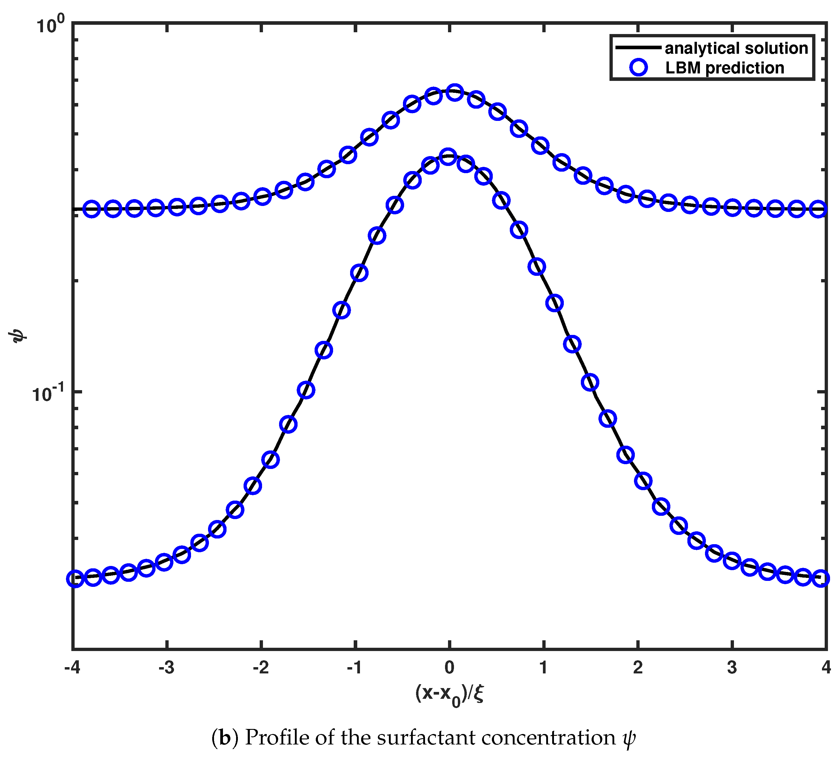
In order to fully characterize and demonstrate the hydrodynamics of an immiscible binary fluid, four main equations, continuity equation, the Navier–Stokes equation and the Cahn–Hilliard equations describing the order parameter and surfactant concentration are used. They can be summarized as follows:

$${\partial }_t\rho +\nabla \left(\rho \mathbf{u}\right)=0$$

(18)

$$\rho ({\partial }_t\mathbf{u}+\mathbf{u}\nabla \mathbf{u})=-\nabla \mathbf{P}+\nabla \left[\mu (\nabla \mathbf{u}+{(\nabla \mathbf{u})}^T)\right]$$

(19)

$${\partial }_t\varphi +\nabla \left(\mathbf{u}\varphi \right)=\nabla (M_{\varphi }\nabla {\mu }_{\varphi })$$

(20)

$${\partial }_t\psi +\nabla \left(\mathbf{u}\psi \right)=\nabla (M_{\psi }\nabla {\mu }_{\psi })$$

(21)

in the above equations, $\rho$, $\mathbf{u}$, $\mathbf{P}$ and $\mu$ are the fluid density, velocity, pressure tensor and dynamic viscosity, respectively. The mobilities for the order parameter, $\varphi$, and the surfactant concenteration, $\psi$, are $M_{\varphi }$ and $M_{\psi }$, respectively.

The symmetrical lattice Boltzmann algorithm is used to solve Equations (18)–(21) to determine the macroscopic properties. The method has second order accuracy in space and time which can recover Navier-stokes accurately. Three particle distribution functions of $f_i(\mathbf{x},\mathbf{t})$, $g_i(\mathbf{x},\mathbf{t})$ and $h_i(\mathbf{x},\mathbf{t})$ are used to describe multiphase flow with surfactant. The time evolution equations for the LB equation for these three distribution functions can be written as:

$$f_i(\mathbf{x}+e_i\Delta t,t+\Delta t)-f_i(\mathbf{x},\Delta t)=-\frac{1}{{\tau }_f}[f_i(\mathbf{x},t)-{f_i}^{eq}(\mathbf{x},\Delta t)]$$

(22)

$$g_i(\mathbf{x}+e_i\Delta t,t+\Delta t)-g_i(\mathbf{x},\Delta t)=-\frac{1}{{\tau }_f}[g_i(\mathbf{x},t)-{g_i}^{eq}(\mathbf{x},\Delta t)]$$

(23)

$$h_i(\mathbf{x}+e_i\Delta t,t+\Delta t)-h_i(\mathbf{x},\Delta t)=-\frac{1}{{\tau }_f}[h_i(\mathbf{x},t)-{h_i}^{eq}(\mathbf{x},\Delta t)]$$

(24)

where $f_{eq}$, $g_{eq}$ and $h_{eq}$ are the equilibrium distribution functions and ${\tau }_f$, ${\tau }_g$ and ${\tau }_h$ are the relaxation times. The macroscopic variables are related to the particle distribution functions as follows:

$$\rho =\sum _{i=0}^8{f}_i(x,t)$$

(25)

$$\rho \mathbf{u}=\sum _{i=0}^8{f}_i(x,t){\mathbf{e}}_i$$

(26)

$$\varphi =\sum _{i=0}^8{g}_i(x,t)$$

(27)

$$\psi =\sum _{i=0}^8{h}_i(x,t)$$

(28)

The relaxation times in the lattice Boltzmann algorithm are related to the physical variables as follows:

$$\upsilon =c_s^2\Delta t({\tau }_f-0.5)$$

(29)

$$M_{\varphi }={\Gamma }_{\varphi }\Delta t({\tau }_g-0.5)$$

(30)

$$M_{\psi }={\Gamma }_{\psi }\Delta t({\tau }_h-0.5)$$

(31)

The equilibrium distribution functions are defined below so as to obtain the continuum equations related to an immiscible binary fluid:

$$\sum _{i=0}^8{f}_i^{eq}{e}_{i\alpha }{e}_{i\beta }=\mathbf{P}+\rho u_{\alpha }{u}_{\beta }$$

(32)

$$\sum _{i=0}^8{g}_i^{eq}{e}_{i\alpha }{e}_{i\beta }={\Gamma }_{\varphi }{\mu }_{\varphi }{\delta }_{\alpha \beta }+\varphi u_{\alpha }{u}_{\beta }$$

(33)

$$\sum _{i=0}^8{h}_i^{eq}{e}_{i\alpha }{e}_{i\beta }={\Gamma }_{\psi }{\mu }_{\psi }{\delta }_{\alpha \beta }+\psi u_{\alpha }{u}_{\beta }$$

(34)

where the subscripts $\alpha$ and $\beta$ represent the components along x and y directions, respectively, and ${\delta }_{\alpha \beta }$ is the Kronecker delta.

3. Model Validation

The proposed method for predicting the profile of surfactant concentration and the order parameter at a planar oil–water interface is tested and the numerically obtained results are compared with analytical solution. A symetrical 2D computational domain with $200\times 10$ lattice cell is considered with an oil phase initially located at 50 < x < 150 and periodic boundary conditions are used for all the boundaries. The remaining parameters are ${\sigma }_0=0.04$, ${\xi }_0=2\Delta x$, $K_{B}T=0.01$, $M_{\varphi }=M_{\psi }=1$, ${\tau }_{\varphi }={\tau }_{\psi }=1$. Two different cases are tested where case one is for $\sigma =0.03$, ${\psi }_b=0.312$ and case two is for $\sigma =0.025$, ${\psi }_b=0.03$. An excellent agreement is observed between our numerical results and the analytical solution, as it is demonstrated in Figure 1 for both the surfactant concentration and the order parameter. The profiles of the surfactant concentration are compatible with the analytical solution even for the relatively large value of $\psi$. This figure confirms that the order parameter is independent of the surfactant loading. It is assumed that surfactant concentration is low in most models. They use this assumption to simplify their models when they mathematically derive their methods. Consequently, their results are largely deviated from analytical solution at the high surfactant concentration [46]. However, an analytical solution is obtained in the proposed model without such an assumption or simplification.

The influence of interfacial thickness on the simulation results is studied. In addition to the result presented in Figure 1, in which interfacial thickness is equal two, we simulate the same setup with similar interfacial tensions and bulk surfactant concentrations but with $\xi =1.14\Delta x$ and $\xi =3\Delta x$. The results are demonstrated in Figure 2. A small deviation is observed for $\xi =1.14\Delta x$ which is similar for a pure mixture binary system while the excellent result is obtined for $\xi =3\Delta x$. The sharp profile of surfactant concentration can be correctly captured across the interface with a reasonably thick interface $\xi =2\Delta x$ demonstrated in Figure 1.

The presence of surfactants changes the interfacial tension. We can control the interfacial tension of droplets with a specific surfactant concentration in the emulation with this proposed model. To exam the accuracy of the model, we consider five samples in which their surfactant concentration and interfacial tension are given in

Table 1. Interfacial tension and surfactant concentration for five different samples. The deviation of the numerical interfacial tension from the given interfacial tension in percentage is defined as error.

Samples	Given Interfacial Tension	Given Bulk Surfactant Concentration	Error
1	0.0389	0.1	2%
2	0.0364	0.3	1.3%
3	0.0330	0.5	0.1%
4	0.0308	0.6	0.6%
5	0.0279	0.7	2.1%

. The samples are selected so that the Langmuir relation is satisfied. These samples can be extracted from experimental results.

An oil droplet resting at the water in a periodic boundary condition is considered for further validation of the model. The computational domain, the interfacial tension and thickness interface without surfactant are $100\times 100$ lattice cell, ${\sigma }_0=0.4$ and $\xi =2\Delta x$, respectively. The radius of droplet R is 30 lattice cell centered in the middle of the computational domain. The resting parameters are $K_{B}T=0.01$, $M_{\varphi }=M_{\psi }=1$, ${\tau }_{\varphi }={\tau }_{\psi }=1$. It must be noted that parameter d is calculated by using Equations (10) and (11) and rearranging them as follows:

$$d=\sqrt{4\left(4Ln\left(2\right)K_{B}T\right)(A-\frac{9{\sigma }^2}{8k})}$$

(35)

where $\sigma$ is the interfacial tension with the presence of surfactant concentration. When the droplet reaches its equilibrium, the interfacial tension is calculated by the Laplace law (for two dimension):

$$\Delta p=\sigma /R$$

(36)

where $\Delta p$ is the pressure difference across the droplet interface. For the five samples, the interfacial tension is obtained by the proposed method and compared with the given interfacial tension at the given surfactant concentration. The deviation of the numerical solution from the given interfacial tension in percentage is calculated and called error in the last column of Table 1. It is observed for all samples, the maximum error is less than $3\%$. The errors in the table show that the model can predict interfacial tension in equilibrium state very good and can be useful when we want to reobtain experimental data in which the availble information are only interfacial tension and surfactant concentration at the bulk.

Surfactant loading at the interface can also be computed numerically and compared with the theory (Equation (17)) for the similar setup and samples when the system reaches the equilibrium. The comparison has been demonstrated in Figure 3 where the good agreement is observed. As it is expected from the analytical expression, a linear relation between the surfactant concentration at bulk and interface is shown.

Time evolution of the surfactant concentration for sample three with a randaom distribution is demonstrated in Figure 4. The surfactant concentration is increased at the interface till it reaches the euqlibrium. In fact, the divergence of chemical potential creates a force and pushs surfactant to attach to the interface. while the surfactant concentration at the interface is increasing, the concentration at the bulk is decreased.

Spurious velocities at the phase interface in many numerical methods in multiphase flows cause artifacts in the simulation. The magnitude of the spurious velocities is proportional to the interfacial tension for a clean droplet in quiescent fluid [47]. The contour of spurious velocity for sample three is shown in Figure 5. Spurious velocities can be decreased by using other collision operators of LBM in which multiple relaxation parameters are used [48].

The larger surfactant concentration in the system, the lower interfacial tension is expected and consequently it leads to bigger reduction of spurious velocities. This behavior is displayed in Figure 6 in which it is also proportional to initial interfacial tension. In this figure, the influence of the interfacial tension on the spurious velocities has been shown. The maximal spurious velocities for three different initial interfacial tension ${\sigma }_0=0.002$, ${\sigma }_0=0.02$ and ${\sigma }_0=0.1$ at bulk surfactant concentration ${\psi }_b=0.5$ are demonstrated. The surfactant concentration itself does not affect spurious velocities as long as the interfacial tension is constant.

The model has a great potential to simulate multiphase flows with the presence of the surfactant. However, the model needs to be more investigated in various fluid flows in which the dynamics of the droplet is important in order to extract the limitations of the model. In this paper, we focus on the validation of the model and the ability of the model to reobtaining numerical interfacial tension. In the future works, the authors intend to study the limitation of the model in various fluid flow.

4. Conclusions

A phase-field model based on free energy is proposed to simulate the surfactant concentration on a binary mixture system. The proposed model allows us to have an analytical solution for the interfacial tension of the system in the presence of the surfactant concentration. The mathematical derivation has been demonstrated. The parameters determining the loading surfactant at the interface can be given as input values in this model. The full control of the system can be obtained using the proposed method in which the only required parameters are the interfacial tension and the bulk surfactant concentration of the system. This model can be used to reobtain the experimental results where there are only these two measured parameters. In fact, this model has promising features that can bridge between numerical and experimental data, which is not available explicitly. The LBM has been used to solve transport equations (the Cahn-Hilliard equation) for the order parameter and the surfactant concentration. The models can be used to simulate both symmetric and asymmetric fluid flow.

The order parameter and the surfactant concentration of numerical results are compared with the analytical solution at a planar oil–water interface. A good agreement is observed in this comparison. Furthermore, the effect of interfacial thickness is investigated, and it is shown the numerical results for the interfacial thickness larger than 2 are in good agreement in comparison with the analytical solution, although for $\xi =1.14\Delta x$ the numerical results are acceptable.

Furthermore, the ability of the method for reobtaining numerical interfacial tension for five different samples are examined and compared with the given initial values for an oil droplet surrounded by water and surfactant. The results show that the obtained interfacial tension from the proposed method agrees well with the given initial interfacial tension. The chemical protentional in the equilibrium obtained by the analytical anumerical solution are compared, and a good agreement is observed. In order to study the ability of the model to predict the time evolution of surfactant, a simulation has been carried out with a random distribution of surfactant concentration. The surfactant moves into the interface. The process has been demonstrated time-dependently.

The maximal value of spurious velocities as a function of initial interfacial tension for contaminated droplets has been shown. It is seen that the spurious velocity of the model is proportional to the interfacial tension. The study of the dynamics of a droplet with the presence of the surfactant is left for future works.

References

1. Teigen, K.E.; Song, P.; Lowengrub, J.; Voigt, A. A diffuse-interface method for two-phase flows with soluble surfactants. J. Comput. Phys. 2011, 230, 375–393. [Google Scholar] [CrossRef] [Green Version]
2. Sjoblom, J. Emulsions and Emulsion Stability: Surfactant Science Series/61; CRC Press: Boca Raton, FL, USA, 2005; Volume 132. [Google Scholar]
3. Stone, H.A.; Stroock, A.D.; Ajdari, A. Engineering flows in small devices: Microfluidics toward a lab-on-a-chip. Annu. Rev. Fluid Mech. 2004, 36, 381–411. [Google Scholar] [CrossRef] [Green Version]
4. Baret, J.C.; Kleinschmidt, F.; El Harrak, A.; Griffiths, A.D. Kinetic aspects of emulsion stabilization by surfactants: A microfluidic analysis. Langmuir 2009, 25, 6088–6093. [Google Scholar] [CrossRef] [PubMed]
5. Mulqueen, M.; Blankschtein, D. Theoretical and experimental investigation of the equilibrium oil- water interfacial tensions of solutions containing surfactant mixtures. Langmuir 2002, 18, 365–376. [Google Scholar] [CrossRef]
6. Zhang, L.; He, L.; Ghadiri, M.; Hassanpour, A. Effect of surfactants on the deformation and break-up of an aqueous drop in oils under high electric field strengths. J. Pet. Sci. Eng. 2015, 125, 38–47. [Google Scholar] [CrossRef] [Green Version]
7. Engblom, S.; Do-Quang, M.; Amberg, G.; Tornberg, A.K. On diffuse interface modeling and simulation of surfactants in two-phase fluid flow. Commun. Comput. Phys. 2013, 14, 879–915. [Google Scholar] [CrossRef] [Green Version]
8. Xu, J.J.; Li, Z.; Lowengrub, J.; Zhao, H. A level-set method for interfacial flows with surfactant. J. Comput. Phys. 2006, 212, 590–616. [Google Scholar] [CrossRef] [Green Version]
9. De Jesus, W.C.; Roma, A.M.; Pivello, M.R.; Villar, M.M.; da Silveira-Neto, A. A 3D front-tracking approach for simulation of a two-phase fluid with insoluble surfactant. J. Comput. Phys. 2015, 281, 403–420. [Google Scholar] [CrossRef]
10. Rinaudo, A.; Raffa, G.M.; Scardulla, F.; Pilato, M.; Scardulla, C.; Pasta, S. Biomechanical implications of excessive endograft protrusion into the aortic arch after thoracic endovascular repair. Comput. Biol. Med. 2015, 66, 235–241. [Google Scholar] [CrossRef]
11. Mendez, V.; Di Giuseppe, M.; Pasta, S. Comparison of hemodynamic and structural indices of ascending thoracic aortic aneurysm as predicted by 2-way FSI, CFD rigid wall simulation and patient-specific displacement-based FEA. Comput. Biol. Med. 2018, 100, 221–229. [Google Scholar] [CrossRef]
12. Seemann, R.; Brinkmann, M.; Pfohl, T.; Herminghaus, S. Droplet based microfluidics. Rep. Prog. Phys. 2011, 75, 016601. [Google Scholar] [CrossRef]
13. Teramoto, T.; Yonezawa, F. Droplet growth dynamics in a water/oil/surfactant system. J. Colloid Interface Sci. 2001, 235, 329–333. [Google Scholar] [CrossRef] [PubMed]
14. Theissen, O.; Gompper, G. Lattice-Boltzmann study of spontaneous emulsification. Eur. Phys. J. B Condens. Matter Complex Syst. 1999, 11, 91–100. [Google Scholar] [CrossRef]
15. Van der Sman, R.; Van der Graaf, S. Diffuse interface model of surfactant adsorption onto flat and droplet interfaces. Rheol. Acta 2006, 46, 3–11. [Google Scholar] [CrossRef]
16. Teng, C.H.; Chern, I.L.; Lai, M.C. Simulating binary fluid-surfactant dynamics by a phase field model. Discret. Contin. Dyn. Syst. B 2012, 17, 1289. [Google Scholar] [CrossRef]
17. Li, Y.; Kim, J. A comparison study of phase-field models for an immiscible binary mixture with surfactant. Eur. Phys. J. B 2012, 85, 1–9. [Google Scholar] [CrossRef]
18. Van der Sman, R.; Meinders, M. Analysis of improved Lattice Boltzmann phase field method for soluble surfactants. Comput. Phys. Commun. 2016, 199, 12–21. [Google Scholar] [CrossRef]
19. Gendre, F.; Ricot, D.; Fritz, G.; Sagaut, P. Grid refinement for aeroacoustics in the lattice Boltzmann method: A directional splitting approach. Phys. Rev. E 2017, 96, 023311. [Google Scholar] [CrossRef] [PubMed]
20. Gorakifard, M.; Salueña, C.; Cuesta, I.; Far, E.K. Analysis of Aeroacoustic Properties of the Local Radial Point Interpolation Cumulant Lattice Boltzmann Method. Energies 2021, 14, 1443. [Google Scholar] [CrossRef]
21. Kian Far, E.; Langer, S. Analysis of the cumulant lattice Boltzmann method for acoustics problems. In Proceedings of the 13th International Conference on Theoretical and Computational Acoustics, Vienna, Austria, 30 July–3 August 2017. [Google Scholar]
22. Gorakifard, M.; Salueña, C.; Cuesta, I.; Kian Far, E. Acoustical analysis of fluid structure interaction using the Cumulant lattice Boltzmann method. In Proceedings of the 16th International Conference for Mesoscopic Methods in Engineering and Science, Edinburgh, UK, 23–26 July 2019. [Google Scholar]
23. Gorakifard, M.; Cuesta, I.; Salueña, C.; Far, E.K. Acoustic wave propagation and its application to fluid structure interaction using the Cumulant Lattice Boltzmann Method. Comput. Math. Appl. 2021, 87, 91–106. [Google Scholar] [CrossRef]
24. Montessori, A.; Lauricella, M.; La Rocca, M.; Succi, S.; Stolovicki, E.; Ziblat, R.; Weitz, D. Regularized lattice Boltzmann multicomponent models for low capillary and Reynolds microfluidics flows. Comput. Fluids 2018, 167, 33–39. [Google Scholar] [CrossRef] [Green Version]
25. O’Connor, J.; Day, P.; Mandal, P.; Revell, A. Computational fluid dynamics in the microcirculation and microfluidics: What role can the lattice Boltzmann method play? Integr. Biol. 2016, 8, 589–602. [Google Scholar] [CrossRef] [Green Version]
26. Pravinraj, T.; Uma, G.; Umapathy, M. A pseudopotential based lattice Boltzmann modeling of electro wetting-on-dielectric for droplet operations. J. Electrost. 2021, 109, 103547. [Google Scholar] [CrossRef]
27. He, Q.; Li, Y.; Huang, W.; Hu, Y.; Li, D.; Wang, Y. Lattice Boltzmann simulations of magnetic particles in a three-dimensional microchannel. Powder Technol. 2020, 373, 555–568. [Google Scholar] [CrossRef]
28. Kian Far, E.; Geier, M.; Kutscher, K.; Krafczyk, M. Implicit Large Eddy Simulation of Flow in a Micro-Orifice with the Cumulant Lattice Boltzmann Method. Computation 2017, 5, 23. [Google Scholar] [CrossRef] [Green Version]
29. Kian Far, E.; Geier, M.; Kutscher, K.; Konstantin, M. Simulation of micro aggregate breakage in turbulent flows by the cumulant lattice Boltzmann method. Comput. Fluids 2016, 140, 222–231. [Google Scholar] [CrossRef]
30. Fattahi, E.; Farhadi, M.; Sedighi, K.; Nemati, H. Lattice Boltzmann simulation of natural convection heat transfer in nanofluids. Int. J. Therm. Sci. 2012, 52, 137–144. [Google Scholar] [CrossRef]
31. Fattahi, E.; Farhadi, M.; Sedighi, K. Lattice Boltzmann simulation of natural convection heat transfer in eccentric annulus. Int. J. Therm. Sci. 2010, 49, 2353–2362. [Google Scholar] [CrossRef]
32. Kian Far, E.; Shirani, E. Simulation of natural convection heat transfer using the lattice boltzmann method in enclosures. In Proceedings of the 17th Annual Conference of Mechanical Engineering, Tehran, Iran, 16 July 2009. [Google Scholar]
33. Fattahi, E.; Pribec, I.; Becker, T. A Novel Lattice Boltzmann Method for Deformable Media. Reactive Flows in Deformable, Complex Media. Math. Forsch. Oberwolfach 2018. [Google Scholar] [CrossRef] [Green Version]
34. Kian Far, E.; Shirani, E.; Geller, S. Fluid structure interaction with using of lattice Boltzmann method. In Proceedings of the 13th Annual and 2nd International Fluid Dynamics Conference, Shiraz, Iran, 26–28 October 2010.
35. Wang, X.; Ban, X.; He, R.; Wu, D.; Liu, X.; Xu, Y. Fluid-solid boundary handling using pairwise interaction model for non-Newtonian fluid. Symmetry 2018, 10, 94. [Google Scholar] [CrossRef]
36. Krafczyk, M.; Tölke, J.; Rank, E.; Schulz, M. Two-dimensional simulation of fluid–structure interaction using lattice-Boltzmann methods. Comput. Struct. 2001, 79, 2031–2037. [Google Scholar] [CrossRef]
37. Kian Far, E.; Geier, M.; Krafczyk, M. Simulation of rotating objects in fluids with the cumulant lattice Boltzmann model on sliding meshes. Comput. Math. Appl. 2018. [Google Scholar] [CrossRef]
38. Kian Far, E. A sliding mesh LBM approach for the simulation of the rotating objects. In Proceedings of the 13th International Conference for Mesoscopic Methods in Engineering and Science, Hamburg, Germany, 22 July 2016. [Google Scholar]
39. Kian Far, E. Simulation of Moving Body in Field Flow and Fluid Structure Interaction with using Lattice Boltzmann Method. Master’s Thesis, Isfahan University of Technology, Isfahan, Iran, 2010. [Google Scholar]
40. Kian Far, E. Turbulent flow simulation of dispersion microsystem with Cumulant lattice Boltzmann method. In Proceedings of the Formula X, Manchester, UK, 24 June 2019. [Google Scholar]
41. Kian Far, E.; Geier, M.; Kutscher, K.; Krafczyk, M. Distributed cumulant lattice Boltzmann simulation of the dispersion process of ceramic agglomerates. J. Comput. Methods Sci. Eng. 2016, 16, 231–252. [Google Scholar] [CrossRef]
42. Fattahi, E.; Waluga, C.; Wohlmuth, B.; Rüde, U.; Manhart, M.; Helmig, R. Lattice Boltzmann methods in porous media simulations: From laminar to turbulent flow. Comput. Fluids 2016, 140, 247–259. [Google Scholar] [CrossRef]
43. Mousavi Tilehboni, S.; Fattahi, E.; Hassanzadeh Afrouzi, H.; Farhadi, M. Numerical simulation of droplet detachment from solid walls under gravity force using lattice Boltzmann method. J. Mol. Liq. 2015, 212, 544–556. [Google Scholar] [CrossRef]
44. Chen, Z.; Shu, C.; Tan, D.; Niu, X.; Li, Q. Simplified multiphase lattice Boltzmann method for simulating multiphase flows with large density ratios and complex interfaces. Phys. Rev. E 2018, 98, 063314. [Google Scholar] [CrossRef]
45. Fei, L.; Yang, J.; Chen, Y.; Mo, H.; Luo, K.H. Mesoscopic simulation of three-dimensional pool boiling based on a phase-change cascaded lattice Boltzmann method. Phys. Fluids 2020, 32, 103312. [Google Scholar] [CrossRef]
46. Liu, H.; Zhang, Y. Phase-field modeling droplet dynamics with soluble surfactants. J. Comput. Phys. 2010, 229, 9166–9187. [Google Scholar] [CrossRef]
47. Van der Sman, R.; Van der Graaf, S. Emulsion droplet deformation and breakup with lattice Boltzmann model. Comput. Phys. Commun. 2008, 178, 492–504. [Google Scholar] [CrossRef]
48. Fard, E.G. A Cumulant LBM approach for Large Eddy Simulation of Dispersion Microsystems. Ph.D. Thesis, Technische Universität Braunschweig, Braunschweig, Germany, 2015. [Google Scholar]
Figure 1. The upper picture demonstrates the profile of the surfactant concentration for a planar oil–water interface located at x 0 = 150 . Circle symbols represent numerical predictions and solid lines are the analytical solutions. The lower picture shows the profile of the solvent composition in which circle symbols represent numerical predictions and the solid line is the analytical solution. Initial interfacial thisckness is ξ = 2 Δ x .
Symmetry 13 01019 g001aSymmetry 13 01019 g001b
Figure 2. The effect of ξ on the profile of the surfactant concentration. The picture demonstrates the profile of the surfactant concentration for a planar oil–water interface located at x 0 = 150 for two different interfacial thicknesses ξ 0 = 1.14 Δ x and ξ 0 = 3 Δ x . Circle symbols represent numerical predictions and solid lines are the analytical solutions.
Symmetry 13 01019 g002
Figure 3. Adsorption isotherm showing surfactant loading of a sphere interface for the five samples where bulk concentrations are 0.1, 0.3, 0.5, 0.6 and 0.7. Symbols represent numerical values, and solid lines are analytical predictions.
Symmetry 13 01019 g003
Figure 4. Time evolution of surfactant concentration for sample three. ParaView as an opensource software has been used for the visualization.
Symmetry 13 01019 g004
Figure 5. Spurious velocity for sample three where ψ b = 0.5 and σ 0 = 0.04 .
Symmetry 13 01019 g005
Figure 6. The maximal value of spurious velocities as a function of σ 0 for contaminated droplets. Three initial interfacial tension σ 0 = 0.002 , σ 0 = 0.02 and σ 0 = 0.1 are used.
Symmetry 13 01019 g006