A Self-Adaptive Reinforcement-Exploration Q-Learning Algorithm

Abstract

Directing at various problems of the traditional Q-Learning algorithm, such as heavy repetition and disequilibrium of explorations, the reinforcement-exploration strategy was used to replace the decayed ε-greedy strategy in the traditional Q-Learning algorithm, and thus a novel self-adaptive reinforcement-exploration Q-Learning (SARE-Q) algorithm was proposed. First, the concept of behavior utility trace was introduced in the proposed algorithm, and the probability for each action to be chosen was adjusted according to the behavior utility trace, so as to improve the efficiency of exploration. Second, the attenuation process of exploration factor ε was designed into two phases, where the first phase centered on the exploration and the second one transited the focus from the exploration into utilization, and the exploration rate was dynamically adjusted according to the success rate. Finally, by establishing a list of state access times, the exploration factor of the current state is adaptively adjusted according to the number of times the state is accessed. The symmetric grid map environment was established via OpenAI Gym platform to carry out the symmetrical simulation experiments on the Q-Learning algorithm, self-adaptive Q-Learning (SA-Q) algorithm and SARE-Q algorithm. The experimental results show that the proposed algorithm has obvious advantages over the first two algorithms in the average number of turning times, average inside success rate, and number of times with the shortest planned route.

1. Introduction

Reinforcement learning (RL), one of methodologies of machine learning, is used to describe and solve how an intelligent agent learns and optimizes the strategy during the interaction with the environment [1]. To be more specific, the intelligent agent acquires the reinforcement signal (reward feedback) from the environment during the continuous interaction with the environment, and adjusts its own action strategy through the reward feedback, aiming at the maximum gain. Different from supervised learning [2] and semi-supervised learning [3], RL does not need to collect training samples in advance, and during the interaction with the environment, the intelligent agent will automatically learn to evaluate the action generated according to the rewards fed back from the environment, instead of being directly told the correct action.

In general, the Markov decision-making process is used by the RL algorithm for environment modeling [4]. Based on whether the transition probability $P$ of the Markov decision-making process in the sequential decision problem is already known, the RL algorithm is divided into two major types [5]: a model-based RL algorithm under known transition probability and a model-free RL algorithm under unknown transition probability, where the former is a dynamic planning method, and the latter mainly includes strategy-based RL method, value function-based RL method, and strategy–value function integrated RL method. The value function-based RL method is an important solution to the model-free Markov problem, and it mainly makes use of Monte Carlo (MC) RL and temporal-difference (TD) RL [6].

As one of most commonly used RL algorithms, the Q-Learning algorithm, which is based on value, reference strategy learning and TD method [7], has been widely applied to route planning, manufacturing and assembly, and dynamic train scheduling [8,9,10]. Many researchers have been dedicated to improving the low exploration efficiency problem of the traditional Q-Learning algorithm. Qiao, J.F. et al. [11] proposed an improved Q-Learning obstacle avoidance algorithm in which Q-Table was substituted with neural network (NN), in an effort to overcome the deficiency of Q-Learning, namely, it was inapplicable under continuous state. Song, Y. et al. [12] applied the artificial potential field to the Q-Learning algorithm, proposed a Q value initialization method, and improved the convergence rate of the Q-Learning algorithm. In [13], a dynamic adjustment algorithm for the exploration factor in $\epsilon \text{-}\mathrm{greedy}$ strategy was raised to improve the exploration-utilization equilibrium problem existing in the practical application of RL method. In the literature [14], a nominal control-based supervised RL route planning algorithm was brought forward, and the tutor supervision was introduced into the Q-Learning algorithm, thus accelerating the algorithm convergence. Andouglas et al. came up with a reward matrix-based Q-Learning algorithm, which satisfies the route planning demand of marine robots [15]. Pauline et al. introduced the concept of partially guided Q-Learning, initialized the Q-Table through the flower pollination algorithm (FPA), and thus optimized the route planning performance of mobile robots [16]. Park, J.H. et al. employed a genetic algorithm to evolve robotic structures as an outer optimization, and it applied a reinforcement learning algorithm to each candidate structure to train its behavior and evaluate its potential learning ability as an inner optimization [17].

It can be seen from the above description that the current research on the improvement of the Q-learning algorithm mainly focuses on two aspects: The first is to study the attenuation law of the exploration factor $\mathit{\epsilon }$ with the increase of the number of training episodes. The second aspect is to adjust the exploration factor $\mathit{\epsilon }$ of the next episode according to the training information of the previous episode. The article creatively proposes the idea of dynamically adjusting the exploration factor of the current episode according to the states accessed times, based on the decayed $\epsilon \text{-}\mathrm{greedy}$ strategy, the concept of behavior utility trace is introduced, and the states accessed list and on-site adaptive dynamic adjustment method are added, so the self-adaptive reinforcement exploration method is realized, and taking the path planning as the application object, the simulation results verify the effectiveness and superiority of the proposed algorithm. The main contributions of the proposed algorithm are as follows: (1) the traditional Q-learning algorithm selects actions randomly according simply to the equal probability method, without considering the differences of actions. In the article, the behavior utility trace is introduced to improve the probability of effective action being randomly selected. (2) In order to better solve the contradiction between exploration and utilization, the article designs the attenuation process of the exploration factor into two stages. The first stage is the exploration stage. The attenuation of the exploration factor is designed slowly to improve the exploration rate. The second stage is the transition from the exploration stage to the utilization stage, which dynamically adjusts the attenuation speed of the exploration factor according to the success rate. (3) In addition, because the exploration factor is fixed in each episode, the agent makes too much exploration near the initial location. The article proposes to record the access times of the current state through the states accessed list, so as to reduce the exploration probability of the states with more accessed times, and improve the exploration rate of the state which is first accessed, so as to improve the radiation range of exploration.

2. Markov Process

2.1. Markov Reward Process (MRP)

In a timing sequence process, if the state at time $t+1$ only depends on the state $S_t$ at time $t$ while unrelated to any state before time $t$, the state $S_t$ at time $t$ is considered with Markov property. If each state in a process is of Markov property, the random process is called Markov process [18].

The key to describing a Markov process lies in the state transition probability matrix, namely, the probability for the transition from the state $S_t=s$ at time $t$ into state $S_{t+1}=s^{\prime }$ at time $t+1$, as shown in Equation (1):

$$P_{s{s}^{\prime }}=p\left[S_{t+1}=s^{\prime }|S_t=s\right]$$

(1)

For a Markov process with $n$ states ($s_1,s_2,\cdots ,s_n$), the state transition probability matrix $P$ from the state $s$ into all follow-up states $s^{\prime }$ is expressed by Equation (2):

$$P=\left[\begin{array}{ccc}{P}_{s_1{s}_1}& \cdots & P_{s_1{s}_n}\\ \cdots & & \cdots \\ P_{s_n{s}_1}& \cdots & P_{s_n{s}_n}\end{array}\right]$$

(2)

In Equation (2), the data in each row of state transition matrix $P$ denote the probability value for the transition from one state into all other $n$ states, and the sum of each row is constantly 1.

An MRP is formed when the reward element is added into a Markov process. An MRP, which is composed of finite state set $S$, state transition probability matrix $P$, reward function $R$ and attenuation factor $\gamma (\gamma \in [0,1\left]\right)$, can be described through a quadruple form $S,P,R,\gamma$.

In an MRP, the sum of all reward attenuations since the initial sampling under a state $S_t$ until the terminal state is called the gain, which is expressed by Equation (3):

$$G_t=R_{t+1}+\gamma R_{t+2}+\cdots +{\gamma }^k{R}_{t+k+1}={\displaystyle \sum }_{i=0}^{\infty }{\gamma }^k{R}_{t+k+1}$$

(3)

In Equation (3), $R_{t+1}$ is the instant reward at time $t+1$, k is the total number of subsequent states from the time $t+1$ until the terminal state, and $R_{t+k+1}$ is the instant reward of terminal state.

The expected gain of a state in the MRP is called value, which is used to describe the importance of a state. The value $v\left(s\right)$ is expressed as shown in Equation (4):

$$v\left(s\right)=E\left[G_t|S_t=s\right]$$

(4)

By unfolding the gain $G_t$ in the value function according to its definition, the expression as shown in Equation (5) can be acquired:

$$v\left(s\right)=E\left[R_{t+1}+\gamma v\left(S_{t+1}\right)|S_t=s\right]$$

(5)

In Equation (5), the expected value of state $S_{t+1}$ at time $t+1$ can be obtained according to the probability distribution at the next time.$s$ denotes the state at the present time, $s^{\prime }$ represents any possible state at the next time, and thus Equation (5) can be written into the following form:

$$v\left(s\right)=R_s+\gamma {\displaystyle \sum }_{s^{\prime }\in S}{P}_{s{s}^{\prime }}v\left(s^{\prime }\right)$$

(6)

Equation (6), which is called Bellman equation in MRP, expresses that the value of a state consists of its reward and the values of subsequent states according to a certain probability and attenuation ratio.

2.2. Markov Decision-Making Process

In addition to the MRP, the RL problem also involves the individual behavior choice. Once the individual behavior choice is included into the MRP, the Markov decision-making process is obtained.

The Markov decision-making process can be described using a quintuple form $\langle S,A,P,R,\gamma ,\rangle$, where its finite behavior set $A$, finite state set $S$ and attenuation factor $\gamma$ are identical with those of the MRP. Different from the MRP, the gain $R$ and state transition probability matrix $P$ in the Markov decision-making process are based on behaviors.

The action $A_t=a$ is chosen at state $S_t=s$, the gain $R_s^a$ at the moment can be expressed by the expected gain $R_{t+1}$ at time $t+1$, and it is mathematically described as shown in Equation (7):

$$R_s^a=E\left[R_{t+1}|S_t=s,A_t=a\right]$$

(7)

The mathematical description of state transition probability $P_{s{s}^{\prime }}^a$from the state $S_t=s$ into the subsequent state $S_{t+1}=s^{\prime }$ is shown in Equation (8):

$$P_{s{s}^{\prime }}^a=P\left[S_{t+1}=s^{\prime }|S_t=s,A_t=a\right]$$

(8)

In the Markov decision-making process, an individual will choose one action from the finite behavior set according to their own recognition of the present state, and the basis for choosing such behavior becomes a strategy and a mapping from one state to action. The strategy is usually expressed by the symbol $\pi$, referring to a distribution based on the behavior set under the given state $s$, namely:

$$\pi \left(a|s\right)=P\left[A_t=a|S_t=s\right]$$

(9)

The state value function $v_{\pi }\left(s\right)$ is used to describe the value generated when the state $s$ abides by a specific strategy $\pi$ in the Markov decision-making process, and it is defined by Equation (10):

$$v_{\pi }\left(s\right)=E\left[G_t|S_t=s\right]$$

(10)

The behavior value function is used to describe the expected gain that can be obtained by executing an action $a$ under the present state $s$ when a specific strategy $\pi$ is followed. As a behavior value is usually based on one state, the behavior value function is also called state-behavior pair value function. The definition of behavior value function $q_{\pi }\left(s,a\right)$ is shown in Equation (11):

$$q_{\pi }\left(s,a\right)=E\left[G_t|S_t=s,A_t=a\right]$$

(11)

By substituting Equation (3) into Equations (10) and (11), respectively, two Bellman expectation Equations (12) and (13) can be acquired:

$$v_{\pi }\left(s\right)=E\left[R_{t+1}+\gamma v_{\pi }\left(S_{t+1}\right)|S_t=s\right]$$

(12)

$$q_{\pi }\left(s,a\right)=E\left[R_{t+1}+\gamma q_{\pi }\left(S_{t+1},A_{t+1}\right)|S_t=s,A_t=a\right]$$

(13)

In the Markov decision-making process, a behavior serves as the bridge of state transition, and the behavior value is closely related to the state value. To be more specific, the state value can be expressed by all behavior values under this state, and the behavior value can be expressed by all state values that the behavior can reach, as shown in Equations (14) and (15), respectively:

$$v_{\pi }\left(s\right)={\displaystyle \sum }_{a\in A}\pi (a|s)q_{\pi }\left(s,a\right)$$

(14)

$$q_{\pi }(s,a)=R_s^a+\gamma {\displaystyle \sum }_{s^{\prime }\in S}{P}_{s{s}^{\prime }}^a{v}_{\pi }\left(s^{\prime }\right)$$

(15)

The following can be obtained by substituting Equation (15) into Equation (14):

$$v_{\pi }\left(s\right)={\displaystyle \sum }_{a\in A}\pi \left(s|a\right)\left(R_s^a+\gamma {\displaystyle \sum }_{s^{\prime }\in S}{P}_{s{s}^{\prime }}^a{v}_{\pi }\left(s^{\prime }\right)\right)$$

(16)

Equation (14) is substituted into Equation (15) to obtain:

$$q_{\pi }\left(s,a\right)=R_s^a+\gamma {\displaystyle \sum }_{s^{\prime }\in S}{P}_{s{s}^{\prime }}^a{\displaystyle \sum }_{a^{\prime }\in A}\pi (a^{\prime }|s^{\prime })q_{\pi }\left(s^{\prime },a^{\prime }\right)$$

(17)

Each strategy corresponds to a state value function, and the optimal strategy naturally corresponds to the optimal state value function. The optimal state value function $v^{*}\left(s\right)$ is defined as the maximum state value function among all strategies, and the optimal behavior value function $q^{*}\left(s,a\right)$ is defined as the maximum behavior value function among all strategies, as shown in Equations (18) and (19), respectively:

$$v^{*}\left(s\right)=\underset{\pi }{max}{v}_{\pi }\left(s\right)$$

(18)

$$q^{*}\left(s,a\right)=\underset{\pi }{max}{q}_{\pi }\left(s,a\right)$$

(19)

From Equations (16) and (17), the optimal state value function and optimal behavior value function can be obtained, as shown in Equations (20) and (21), respectively:

$$v^{*}\left(s\right)=\underset{a}{max}{R}_s^a+\gamma {\displaystyle \sum }_{s^{\prime }\in S}{P}_{s{s}^{\prime }}^a{v}^{*}\left(s^{\prime }\right)$$

(20)

$$q^{*}(s,a)=R_s^a+\gamma {\displaystyle \sum }_{s^{\prime }\in S}{P}_{s{s}^{\prime }}^a{\underset{a}{mqxq}}^{*}(s^{\prime },a^{\prime })$$

(21)

If the optimal behavior value function is known, the optimal strategy can be acquired by directly maximizing the optimal behavior value function $q^{*}\left(s,a\right)$, as shown in Equation (22):

$${\pi }_{*}\left(a|s\right)=\{\begin{array}{cc}1& \mathrm{if} a=\underset{a\in A}{\arg \max q^{*}(s,a)}\\ 0& \mathrm{otherwise}\end{array}$$

(22)

3. Self-Adaptive Reinforcement-Exploration Q-Learning Algorithm

3.1. Q-Learning Algorithm

Compared with the TD reinforcement learning method based on value function and the state–action–reward–state–action (SARSA) algorithm, the iteration of the Q-learning algorithm is a trial-and-error process. One of the conditions for convergence is to try every possible state–action pair many times, and finally learn the optimal control strategy. At the same time, the Q-learning algorithm is an effective reinforcement learning algorithm under the condition of unknown environment. It does not need to establish the environment model, and has the advantages of guaranteed convergence, less parameters and strong exploratory ability. Especially in the field of path planning, which focuses on obtaining the optimal results, the Q-learning algorithm has more advantages, and it is the research hotspot of scholars at present [19]. The Q in Q-Learning algorithm is namely the value $Q_{\left(s,a\right)}$ of state–behavior pair, representing the expected return when the Agent executes the action $a \left(a\in A\right)$ under the state $s \left(s\in S\right)$. The environment will feed back a corresponding instant reward value $r$ according to the behavior a of the Agent. Therefore, the core idea of this algorithm is to use a Q-Table to store all Q values. In the continuous interaction between the Agent and the environment, the expected value (evaluation) is updated through the actual reward $r$obtained by executing the action $a$under the state $s$, and in the end, the action contributing to the maximum return according to the Q-Table is chosen.

Reference strategy TD learning means updating the behavior value with the TD method under the reference strategy condition. The updating method of reference strategy TD learning is shown in Equation (23):

$$V\left(S_t\right)\leftarrow V\left(S_t\right)+\alpha \left(\frac{\pi \left(A_t|S_t\right)}{\mu \left(A_t|S_t\right)}\left(R_{t+1}+\gamma V\left(S_{t+1}\right)\right)-V\left(S_t\right)\right)$$

(23)

In Equation (23), $V\left(S_t\right)$ represents the value assessment of state $S_t$ at time $t$, $V\left(S_{t+1}\right)$ is the value assessment of state $S_{t+1}$ at time $t+1$, $\alpha$ is the learning rate, $\gamma$ is the attenuation factor, $R_{t+1}$ denotes the instant return value at time $t+1$, $\pi \left(A_t|S_t\right)$ is the probability for the target strategy $\pi \left(a|s\right)$ to execute the action $A_t$ under the state $S_{t+1}$, and $\mu \left(A_t|S_t\right)$ is the probability to execute the action $A_t$ under the state $S_{t+1}$ according to the behavior strategy $\mu \left(a|s\right)$. In general, the target strategy $\pi \left(a|s\right)$ chosen is of a certain ability. If $\frac{\pi \left(A_t|S_t\right)}{\mu \left(A_t|S_t\right)}$<1, the probability of the reference strategy choosing the action $A_t$ is smaller than that of the behavior strategy, and the updating amplitude is relatively conservative at the moment. When this ratio is greater than 1, the probability of the reference strategy choosing the action $A_t$ is greater than that for the behavior strategy, and the updating amplitude is relatively bold.

The behavior strategy $\mu$ of reference strategy TD learning method is replaced by the $\epsilon \text{-}\mathrm{greedy}$ strategy based on the value function $Q_{\left(s,a\right)}$, and the target strategy $\pi$ is replaced by the complete greedy strategy based on the value function $Q_{\left(s,a\right)}$, thus forming a Q-Learning algorithm. Q-Learning updates $Q_{\left(S_t,A_t\right)}$ using the time series difference method, and the updating method is expressed by Equation (24):

$$Q\left(S_t,A_t\right)\leftarrow Q\left(S_t,A_t\right)+\alpha \left(R_{t+1}+\gamma Q\left(S_{t+1},A^{\prime }\right)-Q\left(S_t,A_t\right)\right)$$

(24)

In Equation (24), the TD target value $R_{t+1}+\gamma Q\left(S_{t+1},A^{\prime }\right)$ is the Q value of the behavior $A^{\prime }$ generated based on the reference strategy π. Thanks to this updating method, the value of behavior obtained by the state $S_t$ according to the $\epsilon \text{-}\mathrm{greedy}$ strategy will be updated by a certain proportion towards the direction of maximum behavior value determined by the greedy strategy under the state $S_{t+1}$, and will finally converge to the optimal strategy and optimal behavior value. The concrete behavior updating formula of the Q-Learning algorithm is shown in Equation (25):

$$Q\left(S_t,A_t\right)\leftarrow Q\left(S_t,A_t\right)+\alpha \left(R+\gamma \underset{a’}{max}Q\left(S_{t+1},a^{\prime }\right)-Q\left(S_t,A_t\right)\right)$$

(25)

In Equation (25), $a^{\prime }$ is the action acquiring the maximum behavior value under the subsequent states.

3.2. Adaptive Reinforcement-Exploration Strategy Design

3.2.1. Behavior Utility Trace

In order to improve the low exploration efficiency of traditional exploration strategy, in this study, the behavior utility trace [20] was introduced into the probability of action selection, and the self-adaptive reinforcement-exploration strategy was proposed based on the improved $\epsilon \text{-}\mathrm{greedy}$ algorithm.

In the RL, the behavior utility trace was used to record the influence of each state on its subsequent states and to adjust the step size during the state value updating. The behavior utility trace is defined as shown in Equation (26):

$$E_t\left(s\right)=\lambda E_{t-1}\left(s\right)+1\left(S_t=s\right),\lambda \in \left[0,1\right]$$

(26)

In Equation (26), $1\left(S_t=s\right)$ is an expression used to judge true value. It is 1 when and only when $S_t=s$, and 0 under other conditions.

Meanwhile, whether a state is accessed is also an important signal. After an action is executed and transferred to a brand-new state, this, to some extent, indicates that the exploration of action is effective this time. Therefore, the state access function $v\left(s_t\right)$ was used in this study to describe whether a state is accessed as shown in Equation (27):

$$v\left(s_t\right)=\{\begin{array}{cc}0& s_t\in V\\ 1& else\end{array}$$

(27)

In Equation (27), $s_t$ represents the present state, $V$ is the set of accessed states, and the value of $v\left(s_t\right)$ is 1 when and only when this state is accessed for the first time.

By combining instant reward and the features of utility trace and the relationship between whether a state is accessed and the action itself, an action utility trace based on instant reward and state access function was designed in this study as shown in Equation (28):

$$E_t\left(a_i\right)=\{\begin{array}{cc}\lambda E_{t-1}\left(a_i\right)+e\times v\left(s_t\right)\times 1(r_t>0)& a_i=a_{t-1}=a_{t-2}\\ e\times v\left(s_t\right)\times 1(r_t>0)& a_i=a_{t-1}\ne a_{t-2}\\ 0& else\end{array}$$

(28)

In Equation (28), the action $a_i\in A$ is the behavior space of the Agent, $a_{t-1}$ and $a_{t-2}$ are the actions made at the previous time and the time before the previous time, respectively, $r_t$ is the instant reward of the present state, and $e$ value is the exploration incentive value set according to the practical situation. When the same action is continuously chosen for the E value ($E_t\left(a_i\right)$) of action $a_i\in A$, the following will hold: When the instant reward is non-negative and the present state is not accessed, the E value at the present time is obtained by adding $e$ to the attenuation value of E value at the previous time. When the instant reward is negative or the present state is accessed, the E value at the present time is the attenuation value of E value at the previous time. When the action selection is not continuous, the following will be true: The E value at the present time will be $e$ under positive instant reward and 0 under negative instant reward, and the E value will be constantly 0 under other circumstances.

3.2.2. Adaptive Reinforcement-Exploration Strategy

Based on the utility trace introduced, a self-adaptive reinforcement-exploration strategy was put forward in this study. This strategy, which is a symmetric improvement of the $\epsilon \text{-}\mathrm{greedy}$ strategy, was improved mainly from the three following aspects:

• Introduction of the behavior utility trace to improve the probability for different actions to be chosen and to enhance the effectiveness of exploration action.

When the strategy chooses to explore the environment at a certain probability, the probability for each action to be randomly chosen is shown in Equation (29):

$$P\left(a_i\right)=\frac{1+E_{a_i}}{n+{{\displaystyle \sum }}_1^n{E}_{a_j}}$$

(29)

In Equation (29), the action is $a_i\in A$, $E_{a_i}$ is the E value of behavior utility trace for each action, and $n$ is the total number of behavior spaces. When a positive instant reward is obtained by executing one action or the Agent is transferred to a new state, the E value of this action will be enlarged, and so will the probability for it to be chosen. Through such a design, the algorithm can be encouraged to explore in a linear form, thus expanding the radiation range of the initial exploration.

• Real-time adjustment of exploration factor $\epsilon$ in different phases until it meets the objective needs.

As for the adjustment of exploration factor $\epsilon$, the whole attenuation process of $\epsilon$ is divided into two phases. The first phase is the initial training phase of the Agent, in which the Agent almost has no understanding of environmental information and its main task is to explore the environment. In this phase, the attenuation of exploration factor $\epsilon$ should be slightly slow. In this study, the concrete adjustment formula for the exploration factor $\epsilon$ is shown in Equation (30):

$$\begin{array}{cc}{\epsilon }_t=1-sin\left({(\frac{t}{T})}^2\ast \frac{\pi }{2}\right)& t\le \beta T\end{array}$$

(30)

In Equation (30), ${\epsilon }_t$ is the exploration factor at the present time, $t$ is the present number of iteration cycles, $T$ is the maximum number of training cycles of state, and $\beta$ is the self-adaptive exploration factor, with a range of [0, 0.5].

When the iteration cycle satisfies $t>\beta T$, here comes the second phase in which the focus is shifted from the exploration to utilization. In this study, the exploration factor $\epsilon$ was designed into an approximately linear attenuation and gradual stabilization at the set minimum value during this phase. Meanwhile, in order to adjust the attenuation rate according to the practical situation, the concept of success rate proposed in the literature was taken for reference to design the concrete adjustment formula of exploration factor $\epsilon$ in the second phase, as shown in Equation (31):

$${\epsilon }_t=\{\begin{array}{cc}{\epsilon }_1+\frac{t-\beta T}{T_1-\beta T}({\epsilon }_{\min }-{\epsilon }_1)-i\times R& {\epsilon }_1+\frac{t-\beta T}{T_1-\beta T}({\epsilon }_{\min }-{\epsilon }_1)-i\times R\ge {\epsilon }_{\min }\\ {\epsilon }_{\min }& else\end{array}$$

(31)

In Equation (31), ${\epsilon }_1$ is the final value of $\epsilon$ in the first phase, $T_1$ is the target number of episodes of the minimum $\epsilon$, $R$ is the probability of the Agent successfully arriving at the target position in every ten experiments, $i$ is the accelerated utilization factor of the success rate, and ${\epsilon }_{min}$ is the set minimum value of the exploration factor.

Through such a design, the success rate of the Agent becomes higher, and the exploration factor $\epsilon$ attenuates faster, so as to make better use of information and reach the goal of accelerating the convergence while ensuring the algorithm effect.

• Adaptive adjustment of the exploration factor $\epsilon$ of the present action according to the number of access times of the state.

If the traditional exploration strategy is used, although the previous information will be shared in the subsequent iterations, the exploration of the Agent nearby the initial position will be much greater than the exploration nearby the target position. In order to improve the exploration rate nearby the target position and reduce the ineffective exploration nearby the initial position, a dynamic adjustment method was proposed in this study for the exploration factor under a state according to the number of access times of this state. The adjustment formula of exploration factor ${\epsilon }_{cur}$ of the present state within the iteration cycle is shown in Equation (32):

$${\epsilon }_{cur}=\{\begin{array}{cc}{\epsilon }_t+\mu & x=0\\ {\epsilon }_t-\mu sin(\phi x\times \pi /2)& else\end{array}$$

(32)

In Equation (32), ${\epsilon }_t$ is the basic exploration factor of the present state sequence, $\mu$ and $\phi$ are the utilization factors of number of state access times, $x$ is the number of access times of the present state, the maximum value on record is $x_{max}$, and $\phi$ satisfies $\phi x_{max}\le 1$.

3.3. Design of Reward and Penalty Functions

In essence, the RL problem solving means a maximization process of return during the continuous trials and errors and interaction between the Agent and environment. Rightly, as a reward given after the Agent executes an action, the reward function serves as the bridge for the Agent to acquire the environmental information, and its quality has a direct bearing on the convergence or not of the final strategy [21]. The traditional reward function is designed as shown in Equation (33):

$$r=\{\begin{array}{cc}-r_1& \mathrm{collision}\\ r_2& \mathrm{get}\_\mathrm{target}\\ 0& else\end{array}$$

(33)

In Equation (33), both $r_1$ and $r_2$ are positive, collision means that a collision occurs, when the instant reward $-r_1$ is acquired at the moment, and get_target expresses that the Agent successfully arrives at the target position, when the instant reward $r_2$ is harvested. Obviously, the reward function of such a design will be stuck in an obvious problem; the reward values are too sparse, and the Agent will obtain the feedback of reward values only when experiencing a collusion or reaching the target position. However, the Agent fails to obtain any reward feedback under other states, so the Agent has to wander continuously and can be hardly converged. Therefore, the reward density needs to be reasonably increased.

In the reward function designed in this study, any action of Agent would obtain an instant reward. The Agent would acquire an instant reward $r_1$ when colliding, a positive reward $r_2$ when approaching the target, a negative reward $r_3$ when being away from the target, and the final reward $r_4$ when reaching the target position. In the path planning task, the agent needs to reach the target location without collision. Reaching the target location is the ultimate goal and the main task. Therefore, the reward value of $r_4$ should be set to the maximum. The setting of $r_1$ is to avoid collision and can be regarded as a secondary task, so it is less than $r_4$. The setting of $r_2$ and $r_3$ is to avoid that the reward values are too sparse to make the agent unable to reach the target location, which plays an auxiliary role. Therefore, the values of $r_3$ and $r_4$ are set to two orders of magnitude smaller than $r_4$ or $r_1$.The reward function with symmetry designed in this study is shown in Equation (34).

$$r=\{\begin{array}{cc}-r_1& \mathrm{collision}\\ +r_2& \mathrm{close}\_\mathrm{to}\_\mathrm{target}\\ -r_3& \mathrm{far}\_\mathrm{from}\_\mathrm{target}\\ r_4& \mathrm{get}\_\mathrm{target}\end{array}$$

(34)

In Equation (34), $r_1$, $r_2$, $r_3$ and $r_4$ are all positive, close_to_target means approaching the target position, and far_from_target means being far from the target position.

3.4. Algorithm Implementation

The basic idea followed by the proposed SARE-Q algorithm was described as follows: The self-adaptive reinforcement-exploration strategy was used as the behavior selection strategy of the Q-Learning algorithm to improve the environmental exploration efficiency and better balance the contradiction brought by the exploration-utilization problem. Meanwhile, the optimized reward function was combined to enhance the agent-environment interaction efficiency and improve the performance of the original algorithm. The algorithm pseudocode is shown in Algorithm 1:

Algorithm 1 SARE-Q algorithm.

Initialization: The following are initialized: The minimum exploration factor ${\epsilon }_{min}$, the maximum number of iterative episodes $T_{max\_episodes}$, the maximum step size of single episode $T_{max\_steps}$, learning rate $\alpha$, reward attenuation factor $\gamma$, utility trace attenuation factor $\lambda$, exploration incentive value $e$, self-adaptive exploration factor $\beta$, utilization factor $i$ of the success rate, and utilization factors $\mu$ and $\phi$ of access times. The terminal state set $S_T$ is set. For each state $s \left(s\in S\right)$, $a \left(a\in A\right)$, and the initial value of Q-Table is randomly set. The T-Table of state access times is initialized, so is the behavior utility trace table, namely, E-Table.   Loop iteration (for $t=1,2,3\cdots (t<T_{max\_episodes}))$:     Initialize the initial state $s$     Update the basic exploration factor ${\epsilon }_t$     Cycle (for $t=1,2,3\cdots (t<T_{max\_steps})$):       Update the exploration factor ${\epsilon }_{cur}$ in this episode       Choose an action $a$ according to the self-adaptive reinforcement-exploration strategy and Q-Table       Execute the action $a$, and acquire the instant reward $r$ and the state $s1$ at the next time       Update Q-Table, T-Table and E-Table                  $s\leftarrow \mathrm{s}1$     Until reaching the terminal state s or the maximum step size $T_{max\_steps}$ of single episode   Until reaching the maximum number of iterative episodes$T_{max\_episodes}$

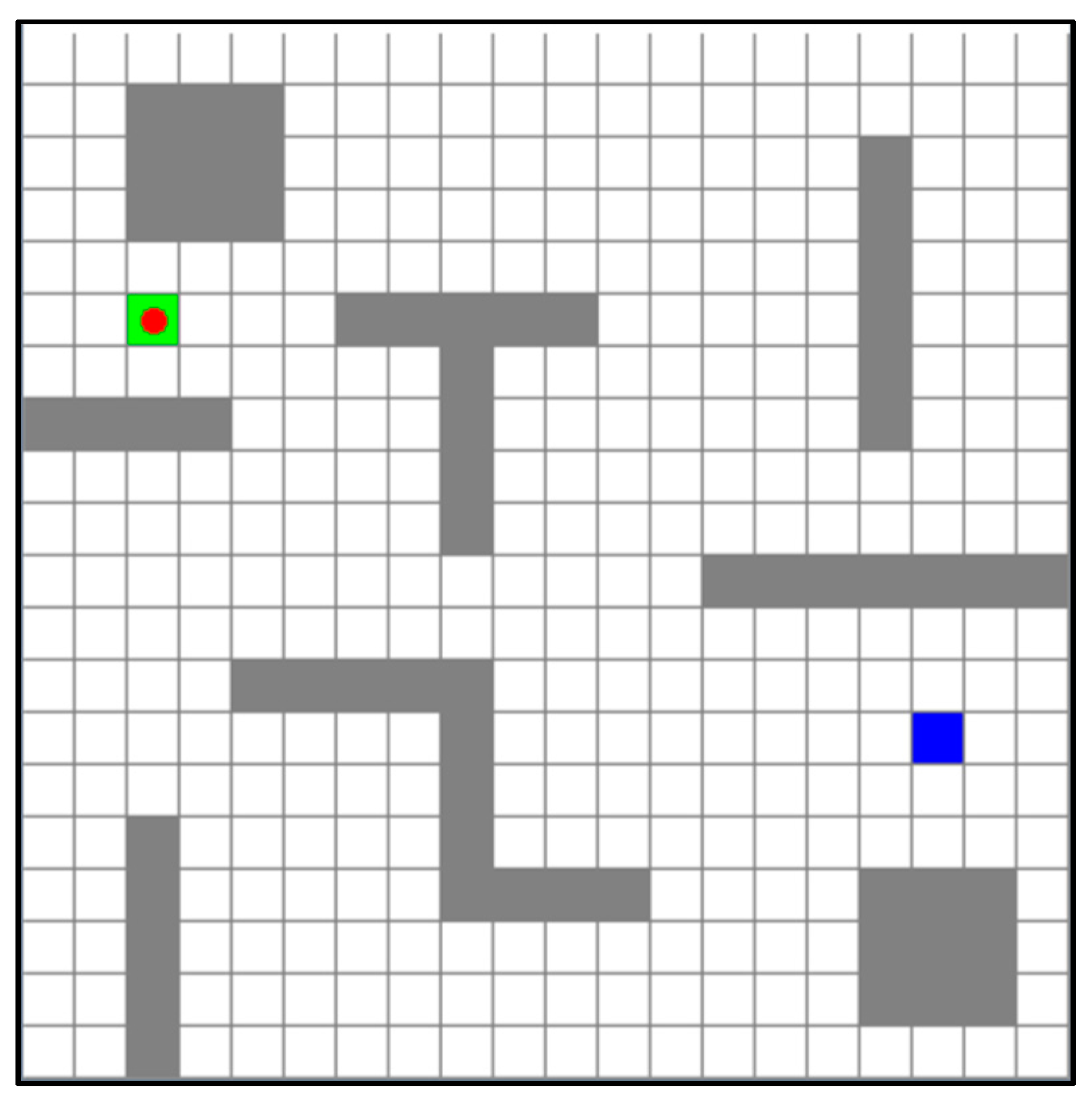
4. Simulation Experiment and Results Analysis

4.1. Simulation Experimental Environment and Parameter Setting

In this study, the simulation experiment was carried out in the n × n symmetric grid map environment commonly used in the route planning experiment. Three experimental scenarios—multi-obstacle grid map environments consisting of 10 × 10, 15 × 15 and 20 × 20 grids, respectively—were designed to verify the Q-Learning algorithm, the self-adaptive Q-Learning (SA-Q) algorithm proposed [22], and the SARE-Q algorithm proposed in this study. Hereby the simulation experimental environment design was introduced by taking the 20 × 20 grid environment for example as shown in Figure 1.

As shown in Figure 1, there were in total 20 × 20 = 400 grids. The grey grids in the figure represented obstacles, and eight different obstacles were set in total. The green grid expressed the initial position of the Agent, with the coordinates of (2,14). The blue grid was the target position of the Agent, with the coordinates of (17,6). The red circle was the Agent. The initial position and target position of the Agent were fixed, and the Agent only moved within the white grids, where neither obstacles nor boundary could gain access. That the Agent was located in different grids represented different states, it could move towards four directions: up, down, left and right, but it could move forward only by the unit grid length towards one direction each time. When the Agent moved towards one direction, if the next target position was an accessible grid, it must be shifted to this grid. If the next target position went beyond the edge or was inaccessible for obstacles, etc., the Agent would stay at the original position.

The experimental simulation platform in this study was as follows: the computer operating system was Windows10, with the CPU of i5-8300H, internal storage of 8 GB, the graphics card of 1050Ti, video memory of 4 GB, conda version of 4.8.4, Python version of 3.5.6, and simulation platform of OpenAI Gym. The related algorithm parameters used were as follows [23]: the initial exploration factor was ${\epsilon }_{\mathrm{init}}=1$, the minimum exploration factor was ${\epsilon }_{min}=0.01$, and through the repeated experiments, the learning rate was set as $\alpha =1.0$, reward attenuation factor as $\gamma =0.9$, the maximum step size of single episode as ${\mathrm{Step}}_{\max }=100$, the maximum number of iterative episodes as $T_{\max \_\mathrm{episodes}}=1000$, the maximum number of exploration episodes as 0.8 times of maximum number of iterative episodes $T_{\max \_\mathrm{episodes}}$, namely 800, utility trace attenuation factor as $\lambda =0.75$, exploration incentive value as $e=1$, self-adaptive exploration factor as $\beta =0.1$, utilization factor of the success rate as $i=0.1$, $\mu$ and $\phi$ for the utilization factor of access times as 0.5 and 0.1, respectively, and $r_1$, $r_2$, $r_3$ and $r_4$ for the reward function as 20, 0, 0.2 and 30, respectively.

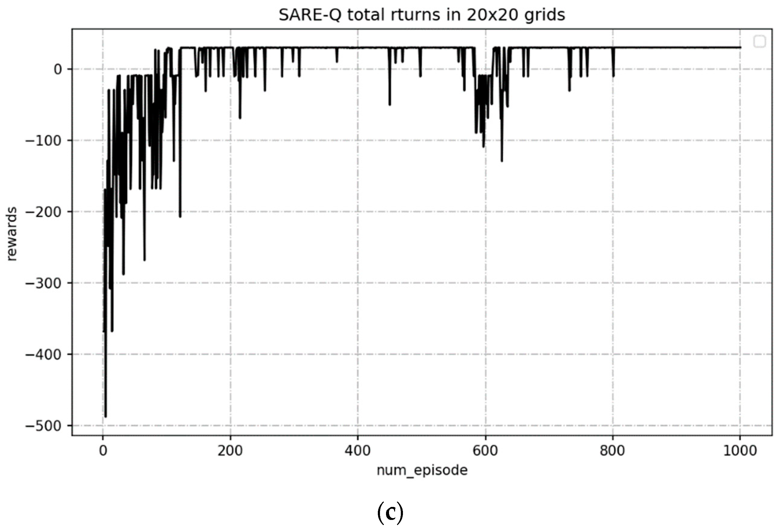
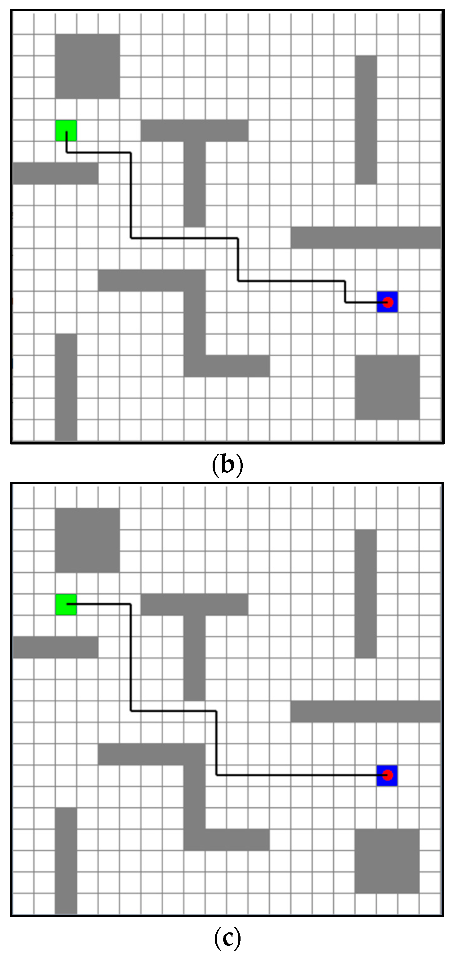
4.2. Simulation Experiment and Result Analysis

In the experimental environment as shown in Figure 1, three different algorithms were used for the route planning, and their typical return curves are displayed in Figure 2, where the x-coordinate denotes the present iterative episode, and y-coordinate represents the total return obtained by each episode.

It could be observed from Figure 2 that in the 20 × 20 grid environment, in comparison with the Q-Learning algorithm and SA-Q algorithm, the Agent could reach the target position earlier by using the SARE-Q algorithm, and the number of times for it to reach the target position was the maximum. From the curve shape, the curves obtained by the Q-Learning algorithm and the SA-Q algorithm were straighter than that obtained by the proposed algorithm after the initial convergence, which is ascribed to the dynamic adjustment of exploration factor $\epsilon$. For any state not accessed or the state accessed for just a few times, the proposed algorithm would reinforce the exploration nearby such state, thus leading to a great curve fluctuation. However, for the other two algorithms, the exploration factor $\epsilon$ was stabilized at a small value in the later iteration phase, and it almost did not fluctuate after being approximately converged.

The optimal routes obtained by 100 route planning experiments using the three different algorithms are shown in Figure 3. It could be shown that all three algorithms could give the shortest routes, among which the number of turning times of the optimal route given by the Q-Learning algorithm was six, that by the SA-Q algorithm was seven and that by the SARE-Q algorithm was four.

The statistical performance results of the three algorithms in executing the route planning task for 100 times are listed in

Table 1. The performance comparison of the three different algorithms in a 20 × 20 grid environment (100 times).

Evaluation Indexes	Q-Learning Algorithm	SA-Q Algorithm	SARE-Q Algorithm
Average operating time (s)	2.047	1.739	1.995
Average number of turning times (times)	9.16	10.22	7.6
Average success rate (%)	30.2	49.7	66
Average step size (step)	23.38	24.44	23.16
Number of times with the shortest route (times)	83	88	92
Number of turning times of the optimal route (times)	6	7	4

. It could be shown from Table 1 that the average operating time of the SARE-Q algorithm differed a little from the SA-Q algorithm and the Q-Learning algorithm. The average number of turning times of the proposed algorithm was the least, and it was much smaller than that of the Q-Learning algorithm and the SA-Q algorithm. As for the average success rate, the proposed algorithm was 16.3% ahead of the SA-Q algorithm, and considerably 35.8% ahead of the Q-Learning algorithm. In the aspects of average step size and number of times with the shortest route, all of the three algorithms might miss the shortest route, but the SARE-Q algorithm was superior to the other two algorithms.

The simulation experiments were implemented in 15 × 15 and 10 × 10 symmetric grid environments, in an effort to explore the influence of different grid environments on the algorithm performance, and the corresponding experimental results are shown in

Table 2. The performance comparison of the three different algorithms in a 15 × 15 grid environment (100 times).

Evaluation Indexes	Q-Learning Algorithm	SA-Q Algorithm	SARE-Q Algorithm
Average operating time (s)	1.43	1.034	1.147
Average number of turning times(times)	9.67	10.32	8.33
Average success rate (%)	41.9	71.5	85.5
Average step size (step)	24.24	24.16	24.04
Number of times with the shortest route (times)	89	93	98
Number of turning times of the optimal route (times)	9	9	7

and

Table 3. The performance comparison of the three different algorithms in a 10 × 10 grid environment (100 times).

Evaluation Indexes	Q-Learning Algorithm	SA-Q Algorithm	SARE-Q Algorithm
Average operating time (s)	0.819	0.629	0.79
Average number of turning times(times)	7.19	7.13	6.1
Average success rate (%)	58.4	70.4	75.2
Average step size (step)	18.1	18.81	18
Number of times with the shortest route (times)	94	99	100
Number of turning times of the optimal route (times)	5	5	4

.

As shown in Table 1, Table 2 and Table 3, all performance indexes of the three algorithms declined with the increase in the number of map grids. During this process, the SA-Q algorithm was comprehensively ahead of the Q-Learning algorithm in terms of performance indexes, though some of its performance indexes were lower than those of Q-Learning algorithm. The SA-Q algorithm was always superior to the other two aspects in terms of operating time. Although the operating time was not as superior as that of the SA-Q algorithm, the other performance indexes of the SARE-Q algorithm were all better than those of the other two algorithms.

5. Conclusions

The SARE-Q algorithm was proposed in this study, in order to tackle the problems of the traditional Q-Learning algorithm, e.g., slow convergence and easy local optimization. In the end, the route planning was simulated on the OpenAI Gym platform. By a symmetric comparison with the Q-Learning algorithm and SA-Q algorithm, the superiority of the proposed SARE-Q algorithm was verified. The following conclusions were obtained through the theoretical study and simulation experiments:

• The problems existing in the Q-Learning algorithm were studied, the behavior utility trace was introduced into the Q-Learning algorithm, and the self-adaptive dynamic exploration factor was combined to put forward a reinforcement-exploration strategy, which substituted the exploration strategy of the traditional Q-Learning algorithm. The simulation experiments of route planning manifest that the SARE-Q algorithm shows advantages, to different extents, over the traditional Q-Learning algorithm and the algorithms proposed in other references in the following aspects: average number of turning times, average inside success rate, average step size, number of times with the shortest planning route, optimal number of turning times of route, etc.
• Though being of a certain complexity, the random environment given in this study is obviously too simple compared with the actual environment. Therefore, the algorithms should be explored under the environment with dynamic obstacles and dynamic target positions in the future. Meanwhile, the algorithm was verified only through the simulation experiments, so the corresponding actual system should be established for the further verification. In addition, the SARE-Q algorithm proposed in this study remains to be further optimized in the aspect of parameter selection. How to optimize the related parameters through intelligent algorithms is the follow-up research content.
• Restricted by the action space and sample space, the traditional RL algorithm is inapplicable to actual scenarios with very large state space and continuous action space. With the integration of deep learning and RL, the deep RL method will overcome the deficiencies of the traditional RL method by virtue of the powerful character representation ability of deep learning technology. The subsequent research content lies in studying the deep RL method and verifying it in the route planning.

References

1. Zhou, X.M.; Bai, T.; Gao, Y.B.; Han, Y. Vision-Based Robot Navigation through Combining Unsupervised Learning and Hierarchical Reinforcement Learning. Sensors 2019, 19, 1576. [Google Scholar] [CrossRef] [Green Version]
2. Miorelli, R.; Kulakovskyi, A.; Chapuis, B.; D’Almeida, O.; Mesnil, O. Supervised learning strategy for classification and regression tasks applied to aeronautical structural health monitoring problems. Ultrasonics 2021, 113, 106372. [Google Scholar] [CrossRef]
3. Faroughi, A.; Morichetta, A.; Vassio, L.; Figueiredo, F.; Mellia, M.; Javidan, R. Towards website domain name classification using graph based semi-supervised learning. Comput. Netw. 2021, 188, 107865. [Google Scholar] [CrossRef]
4. Zeng, J.J.; Qin, L.; Hu, Y.; Yin, Q. Combining Subgoal Graphs with Reinforcement Learning to Build a Rational Pathfinder. Appl. Sci. 2019, 9, 323. [Google Scholar] [CrossRef] [Green Version]
5. Zeng, F.Y.; Wang, C.; Ge, S.S. A Survey on Visual Navigation for Artificial Agents with Deep Reinforcement Learning. IEEE Access 2020, 8, 135426–135442. [Google Scholar] [CrossRef]
6. Li, R.Y.; Peng, H.M.; Li, R.G.; Zhao, K. Overview on Algorithms and Applications for Reinforcement Learning. Comput. Syst. Appl. 2020, 29, 13–25. [Google Scholar] [CrossRef]
7. Luan, P.G.; Thinh, N.T. Hybrid genetic algorithm based smooth global-path planning for a mobile robot. Mech. Based Des. Struct. Mach. 2021, 2021, 1–17. [Google Scholar] [CrossRef]
8. Mao, G.J.; Gu, S.M. An Improved Q-Learning Algorithm and Its Application in Path Planning. J. Taiyuan Univ. Technol. 2021, 52, 91–97. [Google Scholar] [CrossRef]
9. Neves, M.; Vieira, M.; Neto, P. A study on a Q-Learning algorithm application to a manufacturing assembly problem. J. Manuf. Syst. 2021, 59, 426–440. [Google Scholar] [CrossRef]
10. Han, X.C.; Yu, S.P.; Yuan, Z.M.; Cheng, L.J. High-speed railway dynamic scheduling based on Q-Learning method. Control Theory Appl. 2021. Available online: https://kns.cnki.net/kcms/detail/44.1240.TP.20210330.1333.042.html (accessed on 31 March 2021).
11. Qiao, J.F.; Hou, Z.J.; Ruan, X.G. Neural network-based reinforcement learning applied to obstacle avoidance. J. Tsinghua Univ. Sci. Technol. 2008, 48, 1747–1750. [Google Scholar] [CrossRef]
12. Song, Y.; Li, Y.B.; Li, C.H. Initialization in reinforcement learning for mobile robots path planning. Control Theory Appl. 2012, 29, 1623–1628. [Google Scholar]
13. Zhao, Y.N. Research of Path Planning Problem Based on Reinforcement Learning. Master’s Thesis, Harbin Institute of Technology, Harbin, China, 2017. [Google Scholar]
14. Zeng, J.J.; Liang, Z.H. Research of path planning based on the supervised reinforcement learning. Comput. Appl. Softw. 2018, 35, 185–188. [Google Scholar]
15. da Silva, A.G.; dos Santos, D.H.; de Negreiros, A.P.F.; Silva, J.M.; Gonçalves, L.M.G. High-Level Path Planning for an Autonomous Sailboat Robot Using Q-Learning. Sensors 2020, 20, 1550. [Google Scholar] [CrossRef] [PubMed] [Green Version]
16. Low, E.S.; Ong, P.; Cheah, K.C. Solving the optimal path planning of a mobile robot using improved Q-learning. Robot. Auton. Syst. 2019, 115, 143–161. [Google Scholar] [CrossRef]
17. Park, J.H.; Lee, K.H. Computational Design of Modular Robots Based on Genetic Algorithm and Reinforcement Learning. Symmetry 2021, 13, 471. [Google Scholar] [CrossRef]
18. Li, B.H.; Wu, Y.J. Path Planning for UAV Ground Target Tracking via Deep Reinforcement Learning. IEEE Access 2020, 8, 29064–29074. [Google Scholar] [CrossRef]
19. Yan, J.J.; Zhang, Q.S.; Hu, X.P. Review of Path Planning Techniques Based on Reinforcement Learning. Comput. Eng. 2021. [Google Scholar] [CrossRef]
20. Seo, K.; Yang, J. Differentially Private Actor and Its Eligibility Trace. Electronics 2020, 9, 1486. [Google Scholar] [CrossRef]
21. Qin, Z.H.; Li, N.; Liu, X.T.; Liu, X.L.; Tong, Q.; Liu, X.H. Overview of Research on Model-free Reinforcement Learning. Comput. Sci. 2021, 48, 180–187. [Google Scholar]
22. Li, T. Research of Path Planning Algorithm based on Reinforcement Learning. Master’s Thesis, Jilin University, Changchun, China, 2020. [Google Scholar]
23. Li, T.; Li, Y. A Novel Path Planning Algorithm Based on Q-learning and Adaptive Exploration Strategy. In Proceedings of the 2019 Scientific Conference on Network, Power Systems and Computing (NPSC 2019), Guilin, China, 16–17 November 2019; pp. 105–108. [Google Scholar] [CrossRef]
Figure 1. The schematic diagram of 20 × 20 grid environment.
Symmetry 13 01057 g001
Figure 2. The return curve of three different algorithms in a 20 × 20 grid environment: (a) the return curve of the Q-Learning algorithm; (b) the return curve of the SA-Q algorithm; (c) the return curve of the SARE-Q algorithm.
Symmetry 13 01057 g002aSymmetry 13 01057 g002b
Figure 3. The optimal routes planned by three different algorithms in a 20 × 20 grid environment: (a) The optimal route planned by the Q-Learning algorithm; (b) the optimal route planned by the SA-Q algorithm; (c) the optimal route planned by SARE-Q algorithm.
Symmetry 13 01057 g003aSymmetry 13 01057 g003b