Chatter Stability Prediction and Process Parameters’ Optimization of Milling Considering Uncertain Tool Information

Abstract

Stability is the prerequisite of a milling operation, and it seriously depends on machining parameters and machine tool dynamics. Considering that the tool information, including the tool clamping length, feeding direction, and spatial position, has significant effects on machine tool dynamics, this paper presents an efficient method to predict the tool information dependent-milling stability. A generalized regression neural network (GRNN) is established to predict the limiting axial cutting depth, where the machining parameters and tool information are taken as input variables. Moreover, an optimization model is proposed based on the machining parameters and tool information to maximize the material removal rate (MRR), where the GRNN model is taken as the stability constraint. A particle swarm optimization (PSO) algorithm is introduced to solve the optimization model and provide an optimal configuration of the machining parameters and tool information. A case study has been developed to train a GRNN model and establish an optimization model of a real machine tool. Then, effects of the tool information on milling stability were discussed, and an origin-symmetric phenomenon was observed as the feeding direction varied. The accuracy of the solved optimal process parameters corresponding to the maximum MRR was validated through a milling test.

1. Introduction

Regenerative chatter in the milling process is a kind of self-induced vibration caused by time-delayed displacement feedback in the tool-workpiece system. The negative effects induced by the chatter occurrence include serious noise, poor surface quality, increased tool wear, machine tool failure, and so on, seriously limiting the machining quality and efficiency of the milling process [1,2]. Therefore, milling stability has been deeply studied for decades to avoid and suppress the regenerative chatter vibration [3,4,5]. Generally, the stability lobe diagram (SLD) described by different combinations of cutting depth and spindle speed is utilized to select appropriate chatter-free milling parameters to avoid chatter. And the SLD can be usually obtained by performing chatter tests or solving the analytical chatter stability model [6,7].

Quintana [8] performed a large number of milling tests with varying combinations of spindle speed and depth of cut and utilized the measured sound information to plot the SLD. To decrease the number of milling tests, Grossi et al. [9] proposed a spindle ramp-up test to efficiently identify a high number of chatter frequencies and limit axial cutting depths. For theoretical milling stability analysis, the generally used methods are the zero-order approximation (ZOA) method, semi-discretization method (SDM), and full-discretization method (FDM) [10]. Altintas and Budak [11] represented the milling tool-workpiece system as a two-degree freedom system and proposed the ZOA method to compute the SLD. Since the ZOA method needs no iteration and is efficient in predicting the SLD, it has been widely used in milling stability prediction. Insperger et al. [12] initially proposed the SDM in predicting the milling stability, and some improved SDMs were further presented to increase the prediction efficiency. Ding et al. [13] presented the FDM to analyze the responses of milling dynamics, and other researchers introduced different interpolation algorithms to improve the FDM.

Utilizing the aforementioned analytical methods to predict the milling stability needs to obtain the tool point dynamics in advance. In recent years, more and more researchers focusing on the milling stability prediction with uncertain tool point frequency response functions (FRFs) caused by the change in tool-holder combination or tool spatial position. The response coupling substructure analysis (RCSA) method was first proposed by Schmitz, and the improved RCSA methods have been widely used to efficiently predict the tool point FRFs when the tool-holder assembly changed [14]. Law et al. [15] proposed a reduced model substructural synthesis method to efficiently establish a position-dependent multibody dynamic of a machine tool, benefiting rapid predictions of tool point FRFs and milling stability within the whole machine tool working space. Deng et al. [16] establish a backpropagation neural network model to predict the position and feed direction-dependent tool point FRFs, and then study the effects of tool position and feed direction angle on the milling stability.

The groundbreaking research on milling stability provides multiple means of stable process planning in a real machining environment. However, few researchers have considered the effects of the varying tool clamping length on tool point FRFs and thus on the milling stability, and repeated impact tests are still needed to obtain the tool point FRF and identify the tool-holder joint dynamic parameters as the clamping length changed. Smith et al. [17] established the FEM of the high-speed spindle system and studied the effect of the tool length on achievable stable material removal rate (MRR). Duncan [18] put forward that the tool clamping length was an important parameter to improve cutting system dynamics and MRR. Yan et al. [19] adopted uniform distributed spring and damping elements to simulate the holder-tool joint dynamics and identified the spring and damping coefficients per unit contact area to efficiently compute the joint dynamics and tool point FRFs with varying clamping length. The varying tool clamping length can modify the stable zone of the SLD by affecting the tool dynamics, introducing uncertainties in selecting chatter-free machining parameters. Since machining parameters are the dominant factors affecting the machining quality and efficiency, machining parameters’ optimization considering the chatter stability constraint has been researched as the development of the optimization algorithms [20,21,22]. Nevertheless, these optimizations are mainly conducted at a given tool clamping length, spatial position, and feeding direction and ignore the effects of the varying tool information on chatter stability constraint, limiting the selection range of optimal machining parameters for obtaining higher productivity.

Therefore, the purpose of this study is to develop a method to predict the milling stability and obtain optimal process parameters considering the uncertain tool information without repeated impact tests. Initially, typical combinations of tool information including clamping length, feeding direction, and spatial position coordinates are determined by orthogonal experiment method to measure the tool point FRFs through impact testing; then, these tool point FRFs are used to calculate the limiting axial cutting depth (a_plim) under different combinations of machining parameters; on the basis, a generalized regression neural network (GRNN) model whose inputs are the machining parameters and tool information can be trained to predict the a_plim; furthermore, an optimization model for improving the machining efficiency is established by taking the GRNN model to represent the chatter stability constraint, and it can be solved to obtain the optimal combination of machining parameters and tool information.

Henceforth, the following contents of this paper are organized as follows. The principles of predicting the tool information dependent-milling stability are given in Section 2. The detailed information and procedures to establish a process parameters optimization model are provided in Section 3. A case study on the milling process of a real machine tool is described in Section 4. Finally, conclusions from the current research are presented in Section 5.

2. Theoretical Background

2.1. Theoretical Analysis of Milling Chatter Stability

The milling system is generally represented by a two degree of freedom (2-DOF) dynamic model shown in Figure 1a, where the flexible tool is assumed to have two orthogonal degrees of freedom in x and y directions, and the corresponding general equations of motion are expressed in Equation (1).

$$\left\{\begin{array}{l}{m}_x\ddot{x}(t)+c_x\dot{x}(t)+k_{x}x(t)=F_x(t)\\ m_y\ddot{y}(t)+c_y\dot{y}(t)+k_{y}y(t)=F_y(t)\end{array}\right.$$

(1)

where m, c, and k mean the mass, damping, and stiffness, respectively, and the cutting force F_x and F_y can be obtained by Equation (2):

$$\left\{\begin{array}{c}{F}_x(t)\\ F_y(t)\end{array}\right\}=\frac{a_p{K}_{tc}N}{4\pi }\left[\begin{array}{cc}{a}_{xx}& a_{xy}\\ a_{xy}& a_{yy}\end{array}\right]\left\{\begin{array}{c}\Delta x\\ \Delta y\end{array}\right\} =\frac{a_p{K}_{tc}{N}_t}{4\pi }[A]\left\{\begin{array}{c}\Delta x\\ \Delta y\end{array}\right\}$$

(2)

where a_p is the axial depth of cut, N_t is the tool teeth number, K_tc is the tangential cutting force coefficient, and [A] is a matrix containing the average directional coefficients, which can be obtained according to the theory proposed by Altintas and Budak [23]:

$$\begin{array}{l}{a}_{xx}={\left[-\cos \left(2{\phi }_{jl}\right)+2K_{rt}{\phi }_{jl}-K_{rt}\sin \left(2{\phi }_{jl}\right)\right]}_{{\phi }_{st}}^{{\phi }_{ex}}\\ a_{xy}={\left[2{\phi }_{jl}+\sin \left(2{\phi }_{jl}\right)-K_{rt}\cos \left(2{\phi }_{jl}\right)\right]}_{{\phi }_{st}}^{{\phi }_{ex}}\\ a_{yx}={\left[-2{\phi }_{jl}+\sin \left(2{\phi }_{jl}\right)-K_{rt}\cos \left(2{\phi }_{jl}\right)\right]}_{{\phi }_{st}}^{{\phi }_{ex}}\\ a_{yy}={\left[\cos \left(2{\phi }_{jl}\right)+2K_{rt}{\phi }_{jl}+K_{rt}\sin \left(2{\phi }_{jl}\right)\right]}_{{\phi }_{st}}^{{\phi }_{ex}}\end{array}$$

(3)

where K_rt is the ratio of the radial to tangential cutting force coefficient, and φ_st and φ_ex are the start angle and exit angle. Analyzing the dynamics of the milling system in the frequency domain, the dynamic forces can be rewritten in Equation (4):

$$\begin{array}{l}\left\{F\right\}{e}^{i\omega t}=\frac{a_p{K}_{tc}{N}_t}{4\pi }[A]\left(1-e^{-i{\omega }_c\tau }\right)\left[G\left(i{\omega }_c\right)\right]\left\{F\right\}{e}^{i{\omega }_{c}t}\\ \left[G\left(i{\omega }_c\right)\right]=\left[\begin{array}{cc}{G}_{xx}\left(i{\omega }_c\right)& G_{xy}\left(i{\omega }_c\right)\\ G_{yx}\left(i{\omega }_c\right)& G_{yy}\left(i{\omega }_c\right)\end{array}\right]\end{array}$$

(4)

where G(iω_c) is the transfer function matrix which is usually represented by the tool point FRFs in x and y directions as the tool system is more flexible than the workpiece system. Then, the following characteristic equation is derived from Equation (4) to yield the limiting axial cutting depth a_plim.

$$\begin{array}{c}\det \left|I+\mathrm{\Lambda }\left[G_1\left(i{\omega }_c\right)\right]\right|=0\\ \left[G_1\left(i{\omega }_c\right)\right]=[A]\left[G\left(i{\omega }_c\right)\right]\\ \mathrm{\Lambda }=-\frac{a_p{K}_{tc}{N}_t}{4\pi }\left(1-e^{-i{\omega }_c\tau }\right)={\mathrm{\Lambda }}_R+i{\mathrm{\Lambda }}_I\end{array}$$

(5)

where Λ is the eigenvalue and ω_c is the chatter frequency. Ultimately, the a_plim and corresponding spindle speed n can be obtained:

$$\begin{array}{c}{a}_{p\lim }=-\frac{2\pi {\mathrm{\Lambda }}_R\left[1+{\left({\mathrm{\Lambda }}_I/{\mathrm{\Lambda }}_R\right)}^2\right]}{K_{tc}{N}_t}\\ n=\frac{60{\omega }_c}{N_t\left[\left(2k+1\right)\pi -2ta{n}^{-1}\left({\mathrm{\Lambda }}_I/{\mathrm{\Lambda }}_R\right)\right]}\end{array}$$

(6)

According to Equations (1)–(6), the milling stability depends on the transfer function matrix G(iω) containing the tool point FRFs. Thus, the effects of varying tool information on tool point FRFs can further act on the milling stability. Furthermore, the SLDs describing the relationship between the a_plim and n are plotted in Figure 1b, where the red and blue curves represent the SLDs with the tool champing length 60 mm and 50 mm, respectively. Obvious differences between the two SLDs can be observed, indicating the significance of considering the effects of tool clamping length on milling stability prediction and optimization.

2.2. The GRNN Model in Predicting the Tool Clamping Depth-Dependent Milling Stability

Since the tool clamping length, feeding direction, and spatial position can vary in continuous intervals, it is time-consuming and impossible to perform the impact testing at the tool point with each different combination of tool information. Furthermore, the dominant mode number is also uncertain when the tool information changed, adding numerous difficulties in predicting the tool information-dependent modal parameters for recognizing the tool point FRFs and further performing the milling stability analysis. As a consequence, a mathematical model needs to be established to predict the tool information dependent-axial limiting cutting depth a_plim conveniently.

As the generalized regression neural network (GRNN) has great advantages in learning speed and approximation ability compared with the backpropagation neural network (BPNN) and radial basis function neural network (RBFNN), it is first adopted in this research to establish the mathematical mapping relationship between the tool information and axial limiting cutting depth a_plim [24,25]. The typical topologic structure of a GRNN model is described in Figure 2, which was composed of four layers of neurons, including the input layer, pattern layer, summation layer, and output layer [26,27]. The input variable vector X = [X₁, X₂, …, X_p] lies in the input layer, and its dimension p determined the number of neurons. The input vector was processed by linear functions and then transformed into the pattern layer. The neuron number of the pattern layer equaled the number of training samples, and its transfer function was the radial basis function as expressed in Equation (7).

$$p_i=\exp \left[-\frac{{\left(\mathit{X}-{\mathit{X}}_i\right)}^{\mathrm{T}}\left(\mathit{X}-{\mathit{X}}_i\right)}{2{\sigma }^2}\right]$$

(7)

where P_i is the output of the i_th neuron, X_i is the training sample corresponding to the i_th neuron, and the smoothing factor σ is the width coefficient of the Gaussian function.

The summation layer contained two kinds of neurons marked as S_d and S_k, respectively. The first kind S_d is the sum of the output of each neuron in the pattern layer, and the second kind S_k is the weighted sum of the output of each neuron in the pattern layer. S_d and S_k can be computed through Equation (8).

$$\begin{array}{l}{S}_d={\displaystyle \sum _{i=1}^n{p}_i}={\displaystyle \sum _{i=1}^n\exp \left[-\frac{{\left(\mathit{X}-{\mathit{X}}_i\right)}^{\mathrm{T}}\left(\mathit{X}-{\mathit{X}}_i\right)}{2{\sigma }^2}\right]}\\ S_{kj}={\displaystyle \sum _{i=1}^n{y}_{ij}{p}_i=}{\displaystyle \sum _{i=1}^n{y}_{ij}\exp \left[-\frac{{\left(\mathit{X}-{\mathit{X}}_i\right)}^{\mathrm{T}}\left(\mathit{X}-{\mathit{X}}_i\right)}{2{\sigma }^2}\right]}\end{array}$$

(8)

where S_kj means the output of the j_th neuron belonging to the second kind S_k, and y_ij is the expected output of the j_th element corresponding to the i_th training sample.

The neuron number of output layer equaled the dimension of the output vector Y = [Y₁, Y₂, …, Y_m], and the output of the j_th neuron in the output layer is described in Equation (9):

$$y_j=S_{kj}/S_d$$

(9)

It can be seen from Equations (7)–(9) that the hyper-parameter in the GRNN model was the only smoothing factor σ. When σ had a large value, the result of Equation (9) approximated to the mean value of the training sample outputs, reducing the accuracy of the GRNN model. Conversely, a smaller σ made the output of the trained GRNN model more approximate to the real output of the training sample, but an overfitting phenomenon could be observed. Generally, the value of σ was between 0 and 1, and a linear equation was used to find the optimal σ value as shown in Equation (10).

$${\sigma }_t={\sigma }_0-\Delta \sigma \times t\hspace{1em}({\sigma }_t\le {\sigma }_{\max })$$

(10)

where t is the iteration number, Δσ is a constant increment, and σ₀ is an initial value of the smoothing factor, which can be determined by some trial computations. The root mean square error (RMSE) expressed in Equation (11) was used to evaluate the accuracy of the established GRNN model. When the RMSE met the required value, the iteration terminated and the corresponding σ was finally selected to establish the GRNN model.

$$\mathrm{RMSE}=\sqrt{\frac{1}{N_o}{\displaystyle \sum _{j=1}^{N_0}{\left(y_j-y_{jr}\right)}^2}}$$

(11)

where N_o is the number of training samples, and y_jr and y_j represent the real and predicted values of the output variable, respectively.

The machining parameters and tool information, including the spindle speed n, radial cutting width a_e, feed rate per tooth f_z, tool clamping depth l_c, feeding direction angle θ, and spatial coordinates s_x, s_y, and s_z were taken as the input variables, and the limiting axial cutting depth a_plim was taken as the output to predict the tool information dependent-milling stability. On this basis, a GRNN model can be trained according to Equations (7)–(11) to predict the tool information dependent-limiting axial cutting depth.

3. Milling Process Parameters Optimization

Achieving higher productivity with ideal product quality is an important issue that has been focused on in the manufacturing industry. Generally, the machining parameters are taken as the variables to establish an optimization model which does not consider the effects of tool information, limiting the selection region of an optimal combination of spindle speed and axial cutting depth. Thus, an optimization model of a milling process considering the effects of uncertain tool information is provided in this section.

3.1. Variables

The milling efficiency and product quality are highly dependent on the machining parameters and tool-workpiece system dynamics. The machining parameters of a milling process often contain the spindle speed n, axial depth of cut a_p, radial cutting width a_e, and feed rate per tooth f_z. Moreover, the tool-workpiece system dynamics mainly depend on the tool point FRFs which are affected by the tool clamping length l_c, feeding direction angle θ, and spatial position coordinates s_x, s_y, and s_z. Therefore, n, a_p, a_e, f_z, l_c, θ, s_x, s_y, and s_z are taken as the variables.

3.2. Objective Functions

Material removal rate (MRR) stands for the martial volume removed by the tool per unit time in the machining process, and a higher MRR is desired by the industry to improve productivity [28,29]. Then, the MRR is defined as the objective, and it can be described by the machining parameters and tool teeth number N_t shown in Equation (12):

$$\mathrm{MRR}=\frac{n\cdot a_p\cdot a_e\cdot f_z\cdot N_t}{60}$$

(12)

Equation (12) indicates that the MRR is linear to the machining parameters. However, increasing the machining parameters tends to scarify the product quality and cause chatter vibration. For instance, a higher axial depth of cut can improve the MRR, but a chatter vibration may occur and affect the machined surface quality. Therefore, the optimization of MRR should be under the following multiple constraints in Section 3.3.

3.3. Constraint

3.3.1. Milling Stability Constraint

As the milling process should be developed under a chatter-free condition, the axial limiting cutting depth predicted in Section 2.2 is used to describe the milling stability constraint.

$$a_p<a_{p\lim }=f(n,a_e,f_z,l_c,\theta ,s_x,s_y,s_z)$$

(13)

where f(·) stands for the GRNN mathematical model established in Section 2.2.

3.3.2. Power Constraint

The power required by the milling process P_c should not exceed the power output of the machine tool [30].

$$P_c=\frac{C_F{a}_p^{x_F}{f}_z^{y_F}{a}_e^{z_F}{N}_t\pi }{1000D_t{}^{u_F}{\mathrm{n}}^{v_F}}{K}_F\le \eta P_{\max }$$

(14)

where D_t is the tool diameter, η is the machine tool efficiency, and K_F, C_F, x_F, y_F, z_F, u_f, v_f are the corresponding force coefficients.

3.3.3. Surface Roughness Constraint

The surface roughness R_a is an index reflecting the surface quality, and it should meet the technical criteria and requirements of customers. The following empirical formula is commonly used to predict the R_a whose unit is μm, and the specific value of f_z under the unit of mm/z is substituted in Equation (15) [31,32].

$$R_a=318\frac{f_z^2}{\tan ({\theta }_{fa})+\cot ({\theta }_{ba})}<R_{a\max }$$

(15)

where θ_fa and θ_ba are the tool rake angle and relief angle, respectively.

3.3.4. Tool Life Constraint

The tool life is an important constraint considering an economical machining process, and it should not be shorter than the required time proposed by the technologists. In practice, the model proposed by Nefedov and Osipov is often introduced to predict the tool life T_life [30,33].

$$T_{life}={\left(\frac{K_e{C}_v{D}_t^{a-1}}{n{a}_p^e{f}_z^d{a}_e^g{N}_t^w}\right)}^{1/q}\ge T_{\min }$$

(16)

where T_min is the required tool life defined by users and K_v, C_v, a, d, e, g, w, and q are constant coefficients.

3.4. Optimization Model

On the basis of the defined variables, objectives, and constraints, an optimization model for selecting optimal milling process parameters is formed as follows.

$$\begin{array}{l}{Maxmize}: f\left(\mathit{V}\right)=\max \left(\mathrm{MRR}\right)\\ \mathit{V}={\left(\begin{array}{lllllllll}n\hfill & a_p\hfill & a_e\hfill & f_z\hfill & l_c\hfill & \theta \hfill & s_x\hfill & s_y\hfill & s_z\hfill \end{array}\right)}^{\mathrm{T}}\\ s.t. \left\{\begin{array}{c}{\mathit{V}}_{\min }\le \mathit{V}\le {\mathit{V}}_{\max }\\ a_p\le a_{p\lim }\\ R_a\le R_a{}_{\max }\\ T_{life}\le T_{\min }\\ P_c\le \eta P_{\max }\end{array}\right.\end{array}$$

(17)

where V_min and V_max are formed by the minimum and maximum values of each variable, respectively. Particle swarm optimization (PSO) is an algorithm proposed based on the theory of swarm intelligence, which can efficiently search the optimal global particle. Since the PSO has the advantages of simplicity, parallel computing, and fast convergence speed, it has been widely used in the parameter optimization field [34,35]. Therefore, this paper introduced the PSO algorithm to solve the optimization model in Equation (17) to obtain the optimal process parameters. The PSO algorithm is developed through cooperation and competition among the particles. Each individual particle is presented by a D-dimensional position vector (x_i1, x_i2,…, x_id, …, x_iD) which can be updated with the speed vector calculated according to the following algorithm.

$$\left\{\begin{array}{l}{v}_{id}^{k+1}=\omega v_{id}^k+c_1{r}_1\left(P_{bes{t}_{id}}^k-x_{id}^k\right)+c_2{r}_2\left(G_{bes{t}_{id}}^k-x_{id}^k\right)\hfill \\ x_{id}^{k+1}=x_{id}^k+v_{id}^{k+1}\hfill \end{array}\right.$$

(18)

where $v_{\mathit{id}}^k$ and $x_{\mathit{id}}^k$ represent the speed and position of the i_th particle, ω is the inertia weight, c₁ and c₂ are the learning factors, r₁ and r₂ are the random numbers between 0 and 1, and P_best and G_best are the individual and global optimal historical values determined by comparing their fitness values calculated from the fitness function. Generally, ω can be updated using the following Equation (19).

$$\omega ={\omega }_{\max }-k\left({\omega }_{\max }-{\omega }_{\min }\right)/k_{\max }$$

(19)

where the ω_min and ω_max mean the upper and lower limits of the inertial weight.

4. A Case Study

In this section, the proposed milling stability prediction and optimization methods

Considering the comprehensive influences caused by uncertain tool clamping length, feeding direction, and spatial position are applied to a real three-axis vertical machining center shown in Figure 3a. The basic information of the machine tool structure, tool parameters, and milling conditions are described in

Table 1. Specific information of the machine tool.

Item	Symbol	Value	Unit
The tool and workpiece materials		Cemented carbide and steel
Displacement intervals of three directions	[sxmin, sxmax]	[0, 550]	mm
	[symin, symax]	[0, 400]
	[szmin, szmax]	[0, 350]
Intervals of the milling parameters	[nmin, nmax]	[1, 10] × 103	rpm
	[apmin, apmax]	[0, 20]	mm
	[aemin, aemax]	[0, 16]	mm
	[fzmin, fzmax]	[0, 0.4]	mm/z
Tool diameter and tooth number	Dt and Nt	16 and 4	mm
Tool flute length and overall length	lf and lo	46 and 116	mm
Tool clamping length interval	[lcmin, lcmax]	[50, 90]	mm
Tool rake and relief angles	θfa and θba	10 and 15	degree
Rated power and efficiency	Pmax	5.5	Kw
	η	0.85
Power coefficients in Equation (15)	KF	1.0
	CF	129
	xF	0.65
	yF	0.78
	zF	0.86
	uf	0.81
	vf	0.25
Required tool life	Tmin	60	min
Required surface roughness	Ramax	6.4	μm
Tool life coefficients in Equation (17)	Kv	261
	Cv	245
	a	0.64
	d	0.24
	e	0.12
	g	0.26
	w	0.15
	q	0.28

.

4.1. The Milling Stability Prediction by Establishing a GRNN Model

The axial limiting cutting depth a_plim is a significant index to represent the milling stability, and it can be predicted by training a GRNN model under the input variables of machining parameters and tool information. The variation ranges of the input variables n, a_e, f_z, l_c, θ, s_x, s_y, and s_z are listed in Table 1. The sample information of the input and output variables to establish the GRNN model was determined by the following steps.

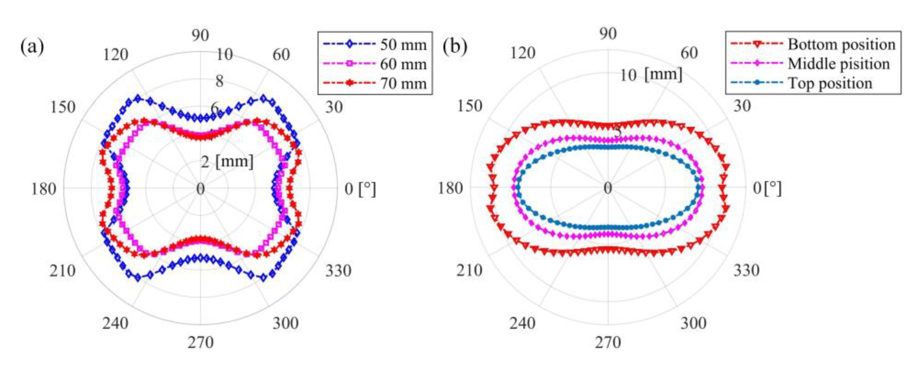
• Step 1: Determine typical combinations of tool information by an orthogonal experiment design method. First, the tool clamping length l_c, feeding direction angle θ, and spatial position coordinates s_x, s_y, and s_z are taken as the factors, and eight levels of each factor are determined within its variation interval and listed in

  Table 2. Specific values for the corresponding levels of each tool parameter.

  Level	lc/mm	θ/°	sx/mm	sy/mm	sz/mm
  1	50	0	70	50	15
  2	56	25	140	100	50
  3	62	50	210	150	100
  4	68	75	280	200	150
  5	74	100	350	250	200
  6	80	125	420	300	250
  7	86	150	490	350	300
  8	90	175	540	385	335

  . Then, an orthogonal table shown in

  Table 3. The orthogonal table of the tool parameters.

  No.	lc	θ	sx	sy	sz	No.	lc	θ	sx	sy	sz	No.	lc	θ	sx	sy	sz
  1	2	1	4	5	6	23	1	3	3	3	3	45	7	2	7	4	6
  2	7	4	5	2	8	24	3	6	4	1	3	46	2	5	8	1	2
  3	4	5	2	6	7	25	4	4	7	3	2	47	5	1	2	8	4
  4	7	3	6	1	7	26	5	2	1	7	3	48	6	1	3	4	7
  5	4	2	5	1	4	27	5	3	4	6	2	49	4	8	3	7	6
  6	8	3	7	5	4	28	3	7	1	4	2	50	8	6	2	4	5
  7	1	2	2	2	2	29	8	2	6	8	1	51	5	4	3	5	1
  8	5	6	5	3	7	30	8	5	1	3	6	52	6	4	2	1	6
  9	2	8	5	4	3	31	6	6	8	7	4	53	8	7	3	1	8
  10	6	8	6	5	2	32	3	2	8	5	7	54	2	6	7	2	1
  11	1	1	1	1	1	33	8	8	4	2	7	55	2	2	3	6	5
  12	4	7	4	8	5	34	3	8	2	3	1	56	3	3	5	8	6
  13	6	3	1	2	5	35	7	7	2	5	3	57	1	8	8	8	8
  14	2	3	2	7	8	36	2	7	6	3	4	58	6	5	7	8	3
  15	7	6	3	8	2	37	8	4	8	6	3	59	5	5	6	4	8
  16	2	4	1	8	7	38	6	7	5	6	1	60	5	8	7	1	5
  17	4	6	1	5	8	39	8	1	5	7	2	61	1	5	5	5	5
  18	7	5	4	7	1	40	7	8	1	6	4	62	3	1	7	6	8
  19	5	7	8	2	6	41	6	2	4	3	8	63	4	3	8	4	1
  20	4	1	6	2	3	42	1	6	6	6	6	64	7	1	8	3	5
  21	1	4	4	4	4	43	1	7	7	7	7
  22	3	5	3	2	4	44	3	4	6	7	5

  is used to determine 64 typical combinations of l_c, θ, s_x, s_y, and s_z. On this basis, the impact testing has been performed at the tool point using the testing instruments in Figure 3a to obtain the corresponding FRFs under each specific combination of l_c, θ, s_x, s_y, and s_z. The tool point FRFs for three different tool clamping lengths are described in Figure 3b, where the dominant mode trends to shit from the higher order to the lower one as the l_c increase. This phenomenon may account for the tool point FRF being dominated by the tool mode when l_c has a smaller value. On the contrary, the tool point FRF is dominated by the spindle mode when l_c has a bigger value.
• Step 2: Determine sample information of the GRNN model. For input machining parameters n, a_e, and f_z, 15 spindle speed values were selected from its interval by an increment of 500 rpm, 8 radial cutting depth values were selected from its interval by an increment of 2 mm, and 10 feed rate per tooth values were selected from its interval By an increment of 0.04 mm/z. Then combining the 64 schemes of l_c, θ, s_x, s_y, and s_z shown in Table 2 and Table 3, 15 × 8 × 10 × 64 = 76,800 combinations of n, a_e, f_z, l_c, θ, s_x, s_y, and s_z were finally determined. At each combination, the computation for obtaining the related a_plim value of a down milling process was developed based on Equations (1)–(6).
• Step 3: Obtain basic structural parameters of a GRNN model. Ninety percent of the 76,800 combinations of n, a_e, f_z, l_c, θ, s_x, s_y, s_z, and a_plim were randomly selected as the training samples, and 10 percent were taken as the testing samples. Then, six values of the smoothing factor σ, including 0.005, 0.01, 0.05, 0.1, 0.5, and 1 were initially determined to perform some trial computations. A computer with 16 G RAM and a 2.6 GHz Intel i7 processor was used to perform the computation in the MATLAB environment, and one complete computation under a specific σ value needed 20.4 s. A smaller RMSE was observed when the smoothing factor σ = 0.05. Thus, σ₀ and Δσ in Equation (10) were determined as 0.05 and 0.0001;
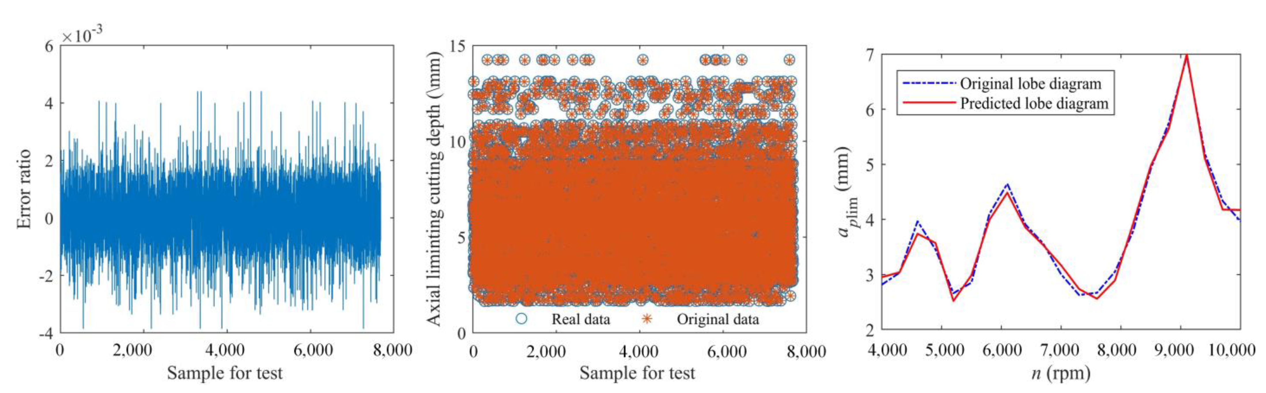
• Step 4: Train and validate the GRNN model for predicting a_plim. Specific values of the 76,800 combinations containing the n, a_e, f_z, l_c, θ, s_x, s_y, and s_z were first normalized. Then, the GRNN model was trained iteratively by modifying σ by an increment of 0.0001. The iteration terminated when the RMSE calculated by Equation (11) was 0.0066, which first met the required 0.01, and the corresponding value of the smoothing factor σ was 0.034. Then, the inputs of the testing samples were used to predict the axial limiting cutting depths by the trained GRNN model. The error percentages between the real and predicted a_plim values are shown in Figure 4, and the maximum error percentage lower than 0.6% verifies the accuracy of the established GRNN model. Furthermore, the original and predicted lobe diagrams are also shown in Figure 4, which are plotted under the given tool information a_e = 12 mm, f_z = 0.08 mm/z, l_c = 60 mm, θ = 30°, s_x = 300 mm, s_y = 200 mm, and s_z = 150 mm. The two lobes have good consistency, which shows that the GRNN model has feasibility in predicting the milling stability.

Figure 4. The error ratios and comparisons between the real and predicted values of a_plim for testing samples, and the comparisons between the original lobe diagram and the one predicted by the established GRNN.

Figure 4. The error ratios and comparisons between the real and predicted values of a_plim for testing samples, and the comparisons between the original lobe diagram and the one predicted by the established GRNN.

With the validated GRNN model, the milling stability for different combinations of machining parameters and tool information can be predicted efficiently. Figure 5a,b describes the limiting axial cutting depth varies with the tool clamping depth and feeding direction angle at different tool spatial positions, respectively. For each figure, an origin-symmetric phenomenon can be observed as the feeding direction angle changes. Furthermore, the a_plim did not decrease monotonously with the decrease in l_c, since the tool point FRFs dominated from the spindle mode to tool mode, and the change in natural frequency caused the shift of the lobe.

4.2. The Optimization of Improving the MRR

The optimization model was established based on the trained GRNN model for predicting the a_plim, and the corresponding coefficients to calculate the power P_c, surface roughness R_a, and tool life T_life are listed in Table 1. The PSO algorithm was used to solve the optimization model under the basic information, including the population size 150, the maximum iteration number was 200, the learning factors c₁ and c₂ were both 1.5, and the initial weights ω_min and ω_max were 0.4 and 0.9, respectively. The position of each particle had nine dimensions representing the variables n, a_p, a_e, f_z, l_c, θ, s_x, s_y, and s_z, and the fitness function was expressed by Equation (12) for computing the optimization objective MRR. Then, the positions and velocities of the particles were randomly initialized and further updated based on Equation (18).

After 79 iterations, the value of MRR trended to a constant 1502.6 mm³/s shown in Figure 6a. The corresponding global optimal particle position and specific information of the constraints are listed in

Table 4. Specific values of the machining parameters and constraints corresponding to the maximum MRR.

n	ap	ae	fz	lc	θ	sx	sy	sz	Pc	Ra	Tlife
r/min	mm	mm	mm/z	mm	degree	mm	mm	mm	Kw	μm	min
4947	7.52	3.55	0.23	74	14	436	325	246	4.67	4.30	75.93

. Analyzing each value of the optimal solution, the maximum MRR was not the product of the maximum values of the n, a_p, a_e and f_z, since it was optimized under the constraints of stability, power, surface roughness, and tool life. A milling test was performed on the vertical machining center with the obtained optimal process parameters to validate the accuracy of the optimization. First, the moving components were driven to move according to the specific optimal values of s_x, s_y, and s_z; then, the tool was inserted into the holder, and the optimal clamping length l_c was kept; finally, the ending milling was performed on the workpiece with the optimal machining parameters n, a_p, a_e, f_z along the optimal feeding direction determined by the value of θ. The force signal of the milling process was measured and transformed into a frequency domain. In Figure 6b, the dominant natural frequencies were the tool passing frequency 331.6 Hz and its harmonics, showing that the milling process was under a stable condition. And the measured surface roughness of the workpiece was 4.36 μm, which is close to the predicted value 4.30 μm and meets the required 6.40 μm of the milling process. Accordingly, the obtained optimal configuration of process parameters can correspond to an efficient and stable milling operation under the requirements of stability, power, surface roughness, and tool life.

5. Conclusions

Stability is the prerequisite of a milling operation, and it is significantly dependent on the tool point dynamics. Since the tool point FRFs are affected by uncertain tool information, including the tool clamping length, feeding direction, and spatial position, this paper proposed a method to predict the tool information dependent-milling stability and obtain optimal process parameters for an efficient milling operation based on the milling stability theory, GRNN model and PSO algorithm. A case study was developed on a real vertical machining center to validate the feasibility of the proposed method.

• The tool clamping length l_c, feeding direction angle θ, and spatial position coordinates s_x, s_y, and s_z were taken as variables to design an orthogonal table with 64 schemes. Then the impact testing was performed at the tool point of each scheme to obtain the tool point FRFs, which showed obvious differences among the dominant natural frequencies and related amplitudes. In addition, the tool point FRFs for different clamping lengths showed that the dominant modes shifted from the tool mode to spindle mode as the tool clamping length increased. Furthermore, typical values of each machining parameter, such as the spindle speed n, radial cutting width a_e, and feed rate per tooth f_z were determined to form different combinations of machining parameters. Then, the tool point FRFs and machining parameters were combined to form different process parameters for computing the corresponding limiting axial cutting depths.
• These different combinations of process parameters and their related values of a_plim were taken as the sample information, 90% of which were determined as the training samples, and 10% were determined as the testing samples. Then, the basic topological structure parameters of the GRNN model were defined, and some values of the smoothing factors were determined to perform some trial computations to find an initial optimal σ. On this basis, the best σ 0.034 was searched through continuous iterations since it first made the RMSE of the training samples below 0.01. The testing samples were used to predict the limiting axial cutting depths with the trained GRNN model, and the maximum error percentage below 0.6% verified the accuracy of the GRNN model. Moreover, the effects of the l_c, θ, s_x, s_y, and s_z on milling stability were analyzed based on the trained GRNN model. The a_plim may increase under some spindle speeds as the l_c decreases and show an origin-symmetric phenomenon when the feeding direction angle θ varies from 0° to 360°.
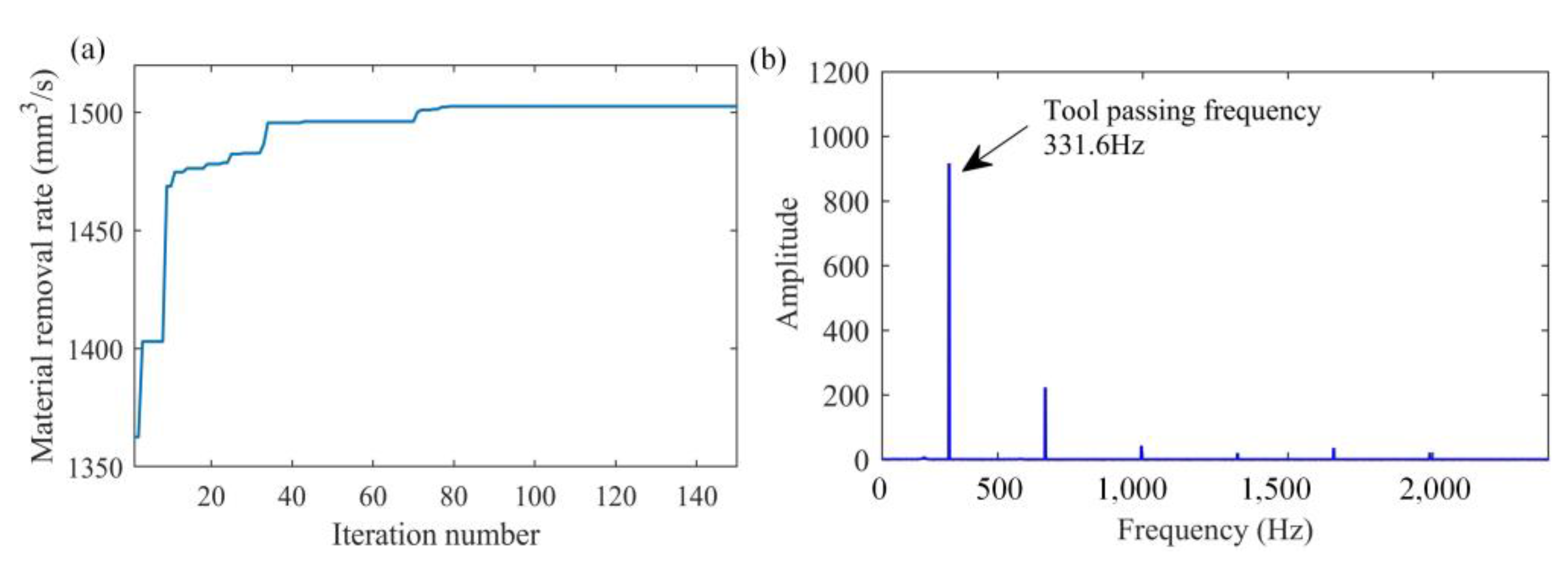
• The process parameters n, a_p, a_e, f_z, l_c, θ, s_x, s_y, and s_z were taken as the variables, and the MRR was taken as the objective to establish an optimization model to obtain an efficient milling operation. The constraints of the optimization model contained the stability, power, surface roughness, and tool life, and the stability constraint was represented by the limiting axial cutting depth predicted using the GRNN model. The PSO algorithm was introduced to solve the established optimization model through continuous iterations, and the obtained optimal combination of process parameters was utilized to perform a milling test. The spectrum analysis of the measured force signal showed that the dominant frequencies were the tool passing frequency and its harmonics and validated the stability of the milling operation. In addition, the measured surface roughness of the workpiece met the requirement of the milling process.

Therefore, the proposed method can be used to predict the tool information dependent-milling stability and further perform a parameters optimization of the milling operation to benefit the process planning. In our further research, the proposed method can be extended to take more objectives and constraints into consideration, making the optimization more adaptive to the real milling process and meet different requirements of customers.

References

1. Li, M.; Zhao, W.; Li, L.; He, N.; Jamil, M. Study the effect of anti-vibration edge length on process stability of milling thin-walled Ti-6Al-4V alloy. Int. J. Adv. Manuf. Technol. 2021, 113, 2563–2574. [Google Scholar] [CrossRef]
2. Niu, J.; Jia, J.; Wang, R.; Xu, J.; Sun, Y.; Guo, D. State dependent regenerative stability and surface location error in peripheral milling of thin-walled parts. Int. J. Mech. Sci. 2021, 196, 106294. [Google Scholar] [CrossRef]
3. Munoa, J.; Beudaert, X.; Dombovari, Z.; Altintas, Y.; Budak, E.; Brecher, C.; Stepan, G. Chatter suppression techniques in metal cutting. CIRP Ann. 2016, 65, 785–808. [Google Scholar] [CrossRef]
4. Dun, Y.; Zhus, L.; Yan, B.; Wang, S. A chatter detection method in milling of thin-walled TC4 alloy workpiece based on auto-encoding and hybrid clustering. Mech. Syst. Signal Process. 2021, 158, 107755. [Google Scholar] [CrossRef]
5. Liu, K.; Zhang, Y.; Gao, X.; Yang, W.; Sun, W.; Dai, F. Improved semi-discretization method based on predictor-corrector scheme for milling stability analysis. Int. J. Adv. Manuf. Technol. 2021, 114, 3377–3389. [Google Scholar] [CrossRef]
6. Hajdu, D.; Insperger, T.; Bachrathy, D.; Stepan, G. Prediction of robust stability boundaries for milling operations with extended multi-frequency solution and structured singular values. J. Manuf. Process. 2017, 30, 281–289. [Google Scholar] [CrossRef] [Green Version]
7. Yamato, S.; Nakanishi, K.; Suzuki, N.; Kakinuma, Y. Development of Automatic Chatter Suppression System in Parallel Milling by Real-Time Spindle Speed Control with Observer-Based Chatter Monitoring. Int. J. Precis. Eng. Manuf. 2021, 22, 227–240. [Google Scholar] [CrossRef]
8. Quintana, G.; Ciurana, J. Chatter in machining processes: A review. Int. J. Mach. Tools Manuf. 2011, 51, 363–376. [Google Scholar] [CrossRef]
9. Grossi, N.; Sallese, L.; Scippa, A.; Campatelli, G. Improved experimental-analytical approach to compute speed-varying tool-tip FRF. Precis. Eng. 2017, 48, 114–122. [Google Scholar] [CrossRef]
10. Zhu, L.; Liu, C. Recent progress of chatter prediction, detection and suppression in milling. Mech. Syst. Signal Process. 2020, 143, 106840. [Google Scholar] [CrossRef]
11. Altintaş, Y.; Budak, E. Analytical Prediction of Stability Lobes in Milling. CIRP Ann. 1995, 44, 357–362. [Google Scholar] [CrossRef]
12. Insperger, T.; Stépán, G.; Hartung, F.; Turi, J. State Dependent Regenerative Delay in Milling Processes. In Proceedings of the ASME 2005 International Design Engineering Technical Conferences and Computers and Information in Engineering Conference (IDETC/CIE), Long Beach, CA, USA, 24–28 September 2005; pp. 1–10. [Google Scholar]
13. Ding, Y.; Zhu, L.; Zhang, X.; Ding, H. A full-discretization method for prediction of milling stability. Int. J. Mach. Tools Manuf. 2010, 50, 502–509. [Google Scholar] [CrossRef]
14. Schmitz, T.L.; Davies, M.A.; Kennedy, M.D. Tool Point Frequency Response Prediction for High-Speed Machining by RCSA. J. Manuf. Sci. Eng. 2001, 123, 700–707. [Google Scholar] [CrossRef]
15. Law, M.; Altintas, Y.; Phani, A.S. Rapid evaluation and optimization of machine tools with position-dependent stability. Int. J. Mach. Tools Manuf. 2013, 68, 81–90. [Google Scholar] [CrossRef]
16. Deng, C.; Feng, Y.; Shu, J.; Huang, Z.; Tang, Q. Prediction of Tool Point Frequency Response Functions Within Machine Tool Work Volume Considering the Position and Feed Direction Dependence. Symmetry 2020, 12, 1073. [Google Scholar] [CrossRef]
17. Smith, S.; Winfough, W.; Halley, J. The Effect of Tool Length on Stable Metal Removal Rate in High Speed Milling. CIRP Ann. 1998, 47, 307–310. [Google Scholar] [CrossRef]
18. Duncan, G.; Tummond, M.; Schmitz, T. An investigation of the dynamic absorber effect in high-speed machining. Int. J. Mach. Tools Manuf. 2005, 45, 497–507. [Google Scholar] [CrossRef] [Green Version]
19. Yan, R.; Cai, F.; Peng, Y.; Wang, Y. Predicting frequency response function for tool point of milling cutters using receptance coupling. J. Huazhong Univ. Sci. Technol. 2013, 41, 1–5. [Google Scholar]
20. Xie, J.; Zhao, P.; Hu, P.; Yin, Y.; Zhou, H.; Chen, J.; Yang, J. Multi-objective feed rate optimization of three-axis rough milling based on artificial neural network. Int. J. Adv. Manuf. Technol. 2021, 114, 1323–1339. [Google Scholar] [CrossRef]
21. Mokhtari, A.; Jalili, M.M.; Mazidi, A. Optimization of different parameters related to milling tools to maximize the allowable cutting depth for chatter-free machining. Proc. Inst. Mech. Eng. Part B J. Eng. Manuf. 2021, 235, 230–241. [Google Scholar] [CrossRef]
22. Yuan, R.; Li, H.; Wang, Q. An enhanced genetic algorithm–based multi-objective design optimization strategy. Adv. Mech. Eng. 2018, 10, 1–6. [Google Scholar] [CrossRef] [Green Version]
23. Budak, E.; Altintas, Y. Analytical prediction of chatter stability in milling—Part I: General formulation; Part II: Application to common milling systems. J. Dyn. Syst. Meas. Control. 1998, 120, 31–36. [Google Scholar] [CrossRef]
24. Liao, X.; Chen, K.; Lu, J. Research on Real-time Control of Machining Surface Quality Stability Based on Wear Monitoring. J. Mech. Eng. 2020, 56, 240–248. [Google Scholar]
25. Khan, A.; Maity, K. A Comprehensive GRNN Model for the Prediction of Cutting Force, Surface Roughness and Tool Wear During Turning of CP-Ti Grade 2. Silicon 2018, 10, 2181–2191. [Google Scholar] [CrossRef]
26. Konakoglu, B. Prediction of geodetic point velocity using MLPNN, GRNN, and RBFNN models: A comparative study. Acta Geod. Geophys. 2021, 56, 271–291. [Google Scholar] [CrossRef]
27. Ceryan, N. Prediction of Young’s modulus of weathered igneous rocks using GRNN, RVM, and MPMR models with a new index. J. Mt. Sci. 2021, 18, 233–251. [Google Scholar] [CrossRef]
28. Sahu, N.K.; Andhare, A.B. Modelling and multiobjective optimization for productivity improvement in high speed milling of Ti–6Al–4V using RSM and GA. J. Braz. Soc. Mech. Sci. Eng. 2017, 39, 5069–5085. [Google Scholar] [CrossRef]
29. Qu, S.; Zhang, M. Optimization for cutting force and material removal rate in milling thin-walled parts. In Proceedings of the 2016 4th International Conference on Advanced Materials and Information Technology Processing (AMITP), Guilin, China, 24–25 September 2016; pp. 461–465. [Google Scholar]
30. Li, C.; Li, L.; Tang, Y.; Zhu, Y.; Li, L. A comprehensive approach to parameters optimization of energy-aware CNC milling. J. Intell. Manuf. 2019, 30, 123–138. [Google Scholar] [CrossRef]
31. Yan, W.; Zhang, H.; Jiang, Z.; Ma, F. Multi-objective optimization model faced to demands of energy saving and high efficiency for CNC machining systems. China Mech. Eng. 2018, 29, 2571–2580. [Google Scholar]
32. Yang, W.-A.; Guo, Y.; Liao, W. Multi-objective optimization of multi-pass face milling using particle swarm intelligence. Int. J. Adv. Manuf. Technol. 2011, 56, 429–443. [Google Scholar] [CrossRef]
33. Nefedov, N.; Osipov, K. Typical Examples and Problems in Metal Cutting and Tool Design; Mir Publishers: Moscow, Russia, 1987. [Google Scholar]
34. Kahouli, O.; Alsaif, H.; Bouteraa, Y.; Ben Ali, N.; Chaabene, M. Power System Reconfiguration in Distribution Network for Improving Reliability Using Genetic Algorithm and Particle Swarm Optimization. Appl. Sci. 2021, 11, 3092. [Google Scholar] [CrossRef]
35. Manh, D.; Quang, P. Safety-enhanced UAV path planning with spherical vector-based particle swarm optimization. Appl. Soft Comput. 2021, 107, 107376. [Google Scholar]
Figure 1. (a) The 2-DOF dynamic model of milling system; (b) the SLD for the milling system with different tool champing lengths.
Symmetry 13 01071 g001
Figure 2. The topologic structure of a GRNN model.
Symmetry 13 01071 g002
Figure 3. (a) The studied vertical machining center and the testing instrument; (b) the Y-directional tool point FRFs with different tool clamping lengths.
Symmetry 13 01071 g003
Figure 5. (a) The values of aplim vary with the tool clamping length lc and feeding direction angle θ; (b) the values of aplim vary with the feeding direction angle θ and tool position sx, sy, and sz.
Symmetry 13 01071 g005
Figure 6. (a) The iteration curve of the PSO algorithm; (b) the frequency spectrum of the cutting force.
Symmetry 13 01071 g006