Article

Abundant Traveling Wave and Numerical Solutions of Weakly Dispersive Long Waves Model

1
Department of Mathematical and Physics, Nanjing Institute of Technology, Nanjing 211167, China
2
Department of Mathematics, Prairie View A & M University, Prairie View, TX 77446, USA
3
Department of Mathematics, Faculty of Science, Jiangsu University, Zhenjiang 212013, China
4
Department of Mathematics, Obour High Institute for Engineering and Technology, Cairo 11828, Egypt
*
Author to whom correspondence should be addressed.
These authors did all this work equally.
Symmetry 2021, 13(6), 1085; https://doi.org/10.3390/sym13061085
Submission received: 28 April 2021 / Revised: 26 May 2021 / Accepted: 1 June 2021 / Published: 17 June 2021

Abstract

:
In this article, plenty of wave solutions of the (2 + 1)-dimensional Kadomtsev–Petviashvili–Benjamin–Bona–Mahony ((2 + 1)-D KP-BBM) model are constructed by employing two recent analytical schemes (a modified direct algebraic (MDA) method and modified Kudryashov (MK) method). From the point of view of group theory, the proposed analytical methods in our article are based on symmetry, and effectively solve those problems which actually possess explicit or implicit symmetry. This model is a vital model in shallow water phenomena where it demonstrates the wave surface propagating in both directions. The obtained analytical solutions are explained by plotting them through 3D, 2D, and contour sketches. These solutions’ accuracy is also tested by calculating the absolute error between them and evaluated numerical results by the Adomian decomposition (AD) method and variational iteration (VI) method. The considered numerical schemes were applied based on constructed initial and boundary conditions through the obtained analytical solutions via the MDA, and MK methods which show the synchronization between computational and numerical obtained solutions. This coincidence between the obtained solutions is explained through two-dimensional and distribution plots. The applied methods’ symmetry is shown through comparing their obtained results and showing the matching between both obtained solutions (analytical and numerical).

1. Introduction

Recently, the phenomenon of shallow water waves has attracted the attention of many researchers in different fields. The flow below the medium pressure surface of the fluid is one of their primary major interests [1,2]. A set of hyperbolic nonlinear evolution equations are the keyword driving this phenomenon [3]. Following Saint-Venard Adéma Jean-Claude Bar de Venat, the shallow water wave equation is named the Saint-Venat equation in bidirectional form [4]. Additionally, the well-known Navier–Stokes equation explains that the conservation of mass means that the vertical velocity scale of the fluid is smaller than the horizontal velocity scale when the horizontal length scale is much larger than the vertical length scale [5,6,7]. Many nonlinear evolution equations have been formulated to demonstrate the waves’ dynamic behavior through shallow water waves. This phenomenon has many applications in engineering and science, such as plasma physics, cosmology, fluid dynamics, electromagnetic theory, acoustics, electrochemistry astrophysics, and so on [8,9,10,11,12,13]. These models have forced many mathematicians and physicists to find suitable tools for finding computational, semi-analytical, and numerical solutions. Distinct schemes have been derived such as the well-known Ψ Ψ -expansion methods, the auxiliary equation method, exponential expansion method, Kudryashov method, sech-tanh expansion method, direct algebraic equation method, Adomian decomposition method, iteration method, Khater methods, B-spline schemes and so on [14,15,16,17,18,19,20]. These techniques have been applied to several nonlinear evolution equations to construct the solutions. Still, there is no unified method that can be used for all models until now. In this scientific race to derive the most general computational technique that can apply to all nonlinear evolution equations, no one has stopped for a single second and asked about the accuracy of all models of the already derived computational schemes.
Sophus Lie has put forth several essential concepts and developed basic tools to study DEs’ group properties. In applied mathematics, he achieved several tangible findings of enormous value. In particular, he established the maximum group of point (local) transformations accepted by the one-dimensional heat equation, discovering the Galilei group’s projective representation. Only lately have these findings been uncovered. Lie’s Theory of continuous groups is based on the well-known Noether theorem on conserved law. Nowadays, several discoveries from Lie are recognized and rediscovered in connection with the present evolution of mathematical and theoretical physics, and we can see the victory of the Lie Theory in all mathematical disciplines.
The fact that Poincare originally founded the Lorentz transformations in 1905, which always leaves Maxwell’s equations, is a key point for identifying Lie Theory because they form a Lie group. In 1909, Bateman and Cunningham found that Maxwell’s equations had been invariant concerning the conformal group, including Lorentz’s subgroup. To build its answers, Bateman used the symmetry of the linear wave equation. These answers were then considered functionally invariant (V.1. Smirnov and S.L. Sobolev, 1932). H. Birkhoff presented several essential concepts for finding accurate PDE solutions. In works by Forsyth and Ames, there are several precise alternatives of two-dimensional nonlinear PDEs. V.P. Ermakov (1890–1900), G.V. Pfeifer (1920–1935), and M.K. Kurensky created the techniques of Lie in Kiev (1930).
In this context, this paper studies the analytical and numerical solutions of the (2 + 1)-D KP-BBM equation. This model is given by [21,22,23]
B x t + B x x + r 1 B 2 x x + r 2 B x x x t + r 3 B y y = 0 ,
where r i , i = 0 , 1 , 2 , 3 are undetermined positive constants while B = B ( ζ , t ) is a space–time function. This function explains the bidirectional propagating water wave surface. Handling Equation (1) through the next transformation B ( ζ , t ) = Y ( ) , = ζ 1 + c t , where c is the wave velocity which converts the PDE into ODE. Integrating the result ODE twice with respect to , and with zero constants of the integration, obtains the next ODE
( c + r 2 + 1 ) Y + r 1 Y 2 + r 2 c Y = 0 .
Using the homogeneous balance principles and the following auxiliary equations for MDA and MK methods [24,25,26,27] for Equation (2), respectively, F ( ) = J 1 + J 2 F ( ) + J 3 F ( ) 2 & Q ( ) = ln ( a ) Q ( ) 2 Q ( ) where J 1 , J 2 , J 3 , a are arbitrary constants to be constructed later; give n = 2 . Thus, the general solutions of Equation (2) are formulated in the following forms
Y = i = n n a i F ( ) i = a 2 F ( ) 2 + a 1 F ( ) + a 2 F ( ) 2 + a 1 F ( ) + a 0 , i = 0 n a i Q ( ) i = a 2 Q ( ) 2 + a 1 Q ( ) + a 0 ,
where a 2 , , a 2 are positive constants.
The paper’s remaining sections are given in the following order; Section 2 constructs novel and accurate solutions of the considered model through the suggested above-mentioned schemes. Section 3 explains the paper’s novelty and contributions. Finally, Section 4 gives the conclusion of the whole paper.

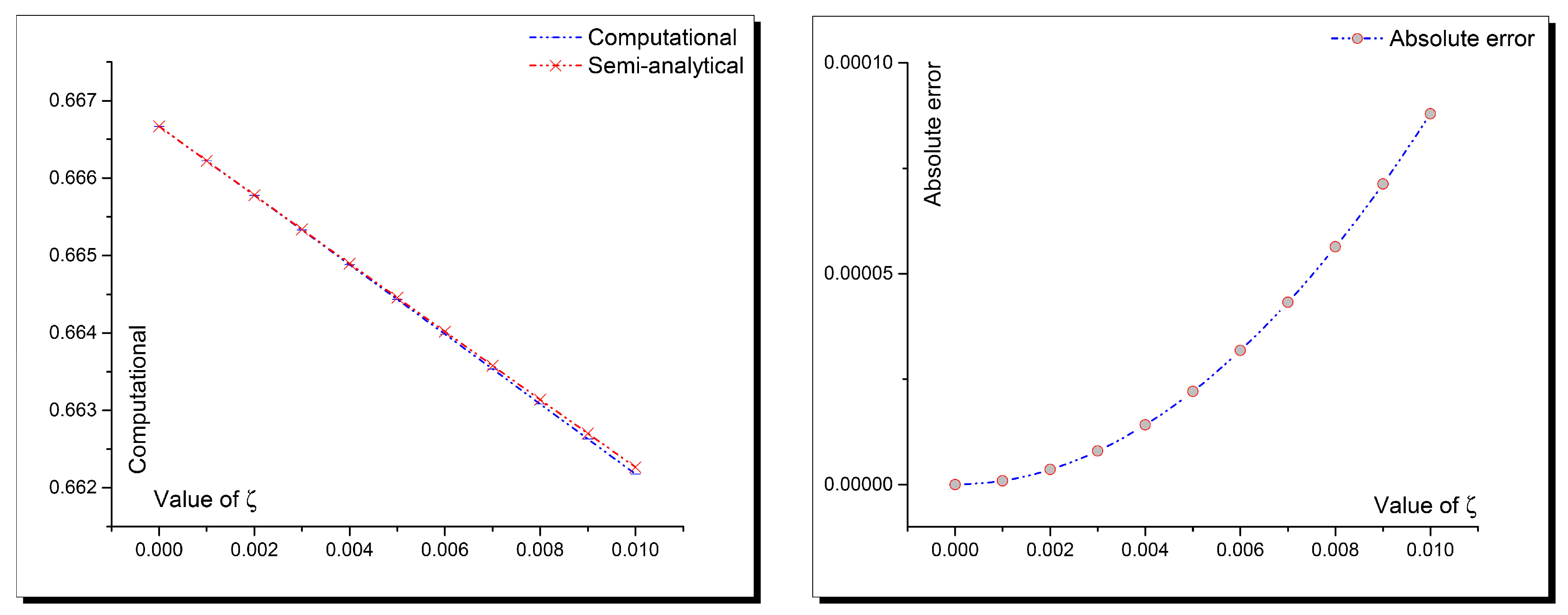
2. Accuracy of Computational Solutions

Applying the MDA and MK methods to Equation (2) to construct traveling wave solutions of the (2 + 1)-D KP-BBM equation is conducted. Additionally, estimate the requested conditions for investigating the numerical solutions of considered model by applying the AD and VI methods as follows:

2.1. MDA Method’s Solutions

Handling Equation (3), through the suggested analytical scheme’ framework, calculates the parameters shown above in the following forms:
Family I
a 0 = J 1 a 1 J 2 , a 2 = a 1 J 3 J 2 , a 1 = 0 , a 2 = 0 , r 1 = 6 c J 2 J 3 r 2 a 1 , r 3 = 4 J 1 c J 3 r 2 c J 2 2 r 2 c 1 .
Family II
a 0 = a 1 J 3 J 2 , a 1 = 0 , a 2 = 0 , a 2 = J 1 a 1 J 2 , r 1 = 6 J 1 c J 2 r 2 a 1 , r 3 = 4 J 1 c J 3 r 2 c J 2 2 r 2 c 1 .
Family III
a 0 = a 1 2 J 1 J 3 + J 2 2 6 J 2 J 3 , a 2 = a 1 J 3 J 2 , a 1 = 0 , a 2 = 0 , r 1 = 6 c J 2 J 3 r 2 a 1 , r 3 = 4 J 1 c J 3 r 2 + c J 2 2 r 2 c 1 .
Family IV
a 0 = a 1 2 J 1 J 3 + J 2 2 6 J 1 J 2 , a 1 = 0 , a 2 = 0 , a 2 = J 1 a 1 J 2 , r 1 = 6 J 1 c J 2 r 2 a 1 , r 3 = 4 J 1 c J 3 r 2 + c J 2 2 r 2 c 1 .
Consequently, the considered model’s traveling solutions are evaluated in the following forms:
For J 1 = 0 , J 2 > 0 , we obtain
B I , 1 ( ζ , t ) = a 1 J 2 e J 2 ( c t + ζ 1 + ϑ ) J 3 e J 2 ( c t + ζ 1 + ϑ ) 1 2 ,
B II , 1 ( ζ , t ) = a 1 e J 2 ( ( c t + ζ 1 + ϑ ) ) J 2 ,
B III , 1 ( ζ , t ) = 2 a 1 J 2 e J 2 ( c t + ζ 1 + ϑ ) 3 J 3 e J 2 ( c t + ζ 1 + ϑ ) 1 2 + a 1 J 2 J 3 e 2 J 2 ( c t + ζ 1 + ϑ ) 6 J 3 e J 2 ( c t + ζ 1 + ϑ ) 1 2 + a 1 J 2 6 J 3 J 3 e J 2 ( c t + ζ 1 + ϑ ) 1 2 .
For J 1 = 0 , J 2 < 0 , we obtain
B I , 2 ( ζ , t ) = a 1 J 3 3 e 2 J 2 ( c t + ζ 1 + ϑ ) J 2 J 3 e J 2 ( c t + ζ 1 + ϑ ) + 1 2 a 1 J 3 2 e 2 J 2 ( c t + ζ 1 + ϑ ) J 3 e J 2 ( c t + ζ 1 + ϑ ) + 1 2 a 1 J 3 e J 2 ( c t + ζ 1 + ϑ ) J 3 e J 2 ( c t + ζ 1 + ϑ ) + 1 2 ,
B II , 2 ( ζ , t ) = a 1 e J 2 ( ( c t + ζ 1 + ϑ ) ) J 3 + a 1 J 3 J 2 a 1 ,
B III , 2 ( ζ , t ) = a 1 J 3 3 e 2 J 2 ( c t + ζ 1 + ϑ ) J 2 J 3 e J 2 ( c t + ζ 1 + ϑ ) + 1 2 + a 1 J 3 e J 2 ( c t + ζ 1 + ϑ ) + 1 + a 1 J 2 6 J 3 a 1 .
For 4 J 1 J 3 > J 2 2 , we obtain
B I , 3 ( ζ , t ) = J 1 a 1 sec 2 1 2 4 J 1 J 3 J 2 2 ( c t + ζ 1 + ϑ ) J 2 a 1 J 2 sec 2 1 2 4 J 1 J 3 J 2 2 ( c t + ζ 1 + ϑ ) 4 J 3 ,
B I , 4 ( ζ , t ) = J 1 a 1 csc 2 1 2 4 J 1 J 3 J 2 2 ( c t + ζ 1 + ϑ ) J 2 a 1 J 2 csc 2 1 2 4 J 1 J 3 J 2 2 ( c t + ζ 1 + ϑ ) 4 J 3 ,
B II , 3 ( ζ , t ) = 4 J 1 a 1 J 3 2 J 2 J 2 cos 1 2 4 J 1 J 3 J 2 2 ( c t + ζ 1 + ϑ ) 4 J 1 J 3 J 2 2 sin 1 2 4 J 1 J 3 J 2 2 ( c t + ζ 1 + ϑ ) 2 a 1 J 2 J 3 J 2 cos 1 2 4 J 1 J 3 J 2 2 ( c t + ζ 1 + ϑ ) 4 J 1 J 3 J 2 2 sin 1 2 4 J 1 J 3 J 2 2 ( c t + ζ 1 + ϑ ) 2 ,
B II , 4 ( ζ , t ) = 4 J 1 a 1 J 3 2 J 2 4 J 1 J 3 J 2 2 cos 1 2 4 J 1 J 3 J 2 2 ( c t + ζ 1 + ϑ ) J 2 sin 1 2 4 J 1 J 3 J 2 2 ( c t + ζ 1 + ϑ ) 2 a 1 J 2 J 3 4 J 1 J 3 J 2 2 cos 1 2 4 J 1 J 3 J 2 2 ( c t + ζ 1 + ϑ ) J 2 sin 1 2 4 J 1 J 3 J 2 2 ( c t + ζ 1 + ϑ ) 2 ,
B III , 3 ( ζ , t ) = 2 J 1 a 1 3 J 2 + J 1 a 1 sec 2 1 2 4 J 1 J 3 J 2 2 ( c t + ζ 1 + ϑ ) J 2 a 1 J 2 sec 2 1 2 4 J 1 J 3 J 2 2 ( c t + ζ 1 + ϑ ) 4 J 3 + a 1 J 2 6 J 3 ,
B III , 4 ( ζ , t ) = 2 J 1 a 1 3 J 2 + J 1 a 1 csc 2 1 2 4 J 1 J 3 J 2 2 ( c t + ζ 1 + ϑ ) J 2 a 1 J 2 csc 2 1 2 4 J 1 J 3 J 2 2 ( c t + ζ 1 + ϑ ) 4 J 3 + a 1 J 2 6 J 3 ,
B IV , 1 ( ζ , t ) = a 1 J 2 6 J 1 + 4 J 1 a 1 J 3 2 J 2 J 2 4 J 1 J 3 J 2 2 tan 1 2 4 J 1 J 3 J 2 2 ( c t + ζ 1 + ϑ ) 2 2 a 1 J 3 J 2 4 J 1 J 3 J 2 2 tan 1 2 4 J 1 J 3 J 2 2 ( c t + ζ 1 + ϑ ) + a 1 J 3 3 J 2 ,
B IV , 2 ( ζ , t ) = a 1 J 2 6 J 1 + 4 J 1 a 1 J 3 2 J 2 J 2 4 J 1 J 3 J 2 2 cot 1 2 4 J 1 J 3 J 2 2 ( c t + ζ 1 + ϑ ) 2 2 a 1 J 3 J 2 4 J 1 J 3 J 2 2 cot 1 2 4 J 1 J 3 J 2 2 ( c t + ζ 1 + ϑ ) + a 1 J 3 3 J 2 .
where ζ = x , y , ζ 1 = x + y .

Semi-Analytical Solutions

  • Applying AD method [28,29] for Equation (2) with the following initial and boundary conditions Y ( 0 ) = 6 e 2 x 2 e 2 x 1 2 , Y ( 0 ) = 4 9 gives the following solutions
    Y 0 = 2 3 4 9 ,
    Y 1 = 32 4 243 40 3 81 + 4 2 9 ,
    Y 2 = 1024 7 45927 + 320 6 2187 392 5 1215 + 20 4 81 ,
    Y 3 = 4096 10 2657205 16384 9 1240029 + 1888 8 45927 17264 7 229635 + 2008 6 10935 512 5 1215 + 32 4 81 .
    Thus, the semi-analytical solutions of the (2 + 1)-D KP-BBM equation is given by
    Y A p p r o x . = 4096 10 2657205 16384 9 1240029 + 1888 8 45927 22384 7 229635 + 3608 6 10935 904 5 1215 + 188 4 243 40 3 81 + 4 2 9 4 9 + 2 3 + .
  • Applying the variational iteration method [30] for Equation (1) with the following initial condition B ( ζ , 0 ) = 6 e 2 ( ζ 1 ) 2 e 2 ( ζ 1 ) 1 2 gives the following solutions:
    B 1 ( ζ , t ) = 6 ( sinh ( ζ 1 ) + 3 cosh ( ζ 1 ) ) 4 288 t ( 3 sinh ( 2 ( ζ 1 ) ) + 5 cosh ( 2 ( ζ 1 ) ) 6 ) ( sinh ( ζ 1 ) + 3 cosh ( ζ 1 ) ) 6 ,
    B 2 ( ζ , t ) = 1 ( sinh ( ζ 1 ) + 3 cosh ( ζ 1 ) ) 14 ( 3456 t ( 215654400 t 2 ( sinh ( ζ 1 ) + 3 × cosh ( ζ 1 ) ) 2 ( 3 ( 4608 t ( 7 2904 t ) + 88552 sinh ( 2 ( ζ 1 ) ) + 32680 × sinh ( 4 ( ζ 1 ) ) 50826 sinh ( 6 ( ζ 1 ) ) + 5055 sinh ( 8 ( ζ 1 ) ) + 160 ) + 40 ( 36 t ( 12384 t + 7 ) + 3997 ) cosh ( 2 ( ζ 1 ) ) 8 ( 1224 t ( 192 t + 17 ) 10817 ) × cosh ( 4 ( ζ 1 ) ) + 6 ( 36 t ( 4 ( 12384 t + 7 ) sinh ( 2 ( ζ 1 ) ) 40 ( 192 t + 17 ) sinh ( 4 ( ζ 1 ) ) + 189 sinh ( 6 ( ζ 1 ) ) ) + 65 ( 108 t 379 ) cosh ( 6 ( ζ 1 ) ) ) + 15043 cosh ( 8 ( ζ 1 ) ) ) ) ) .

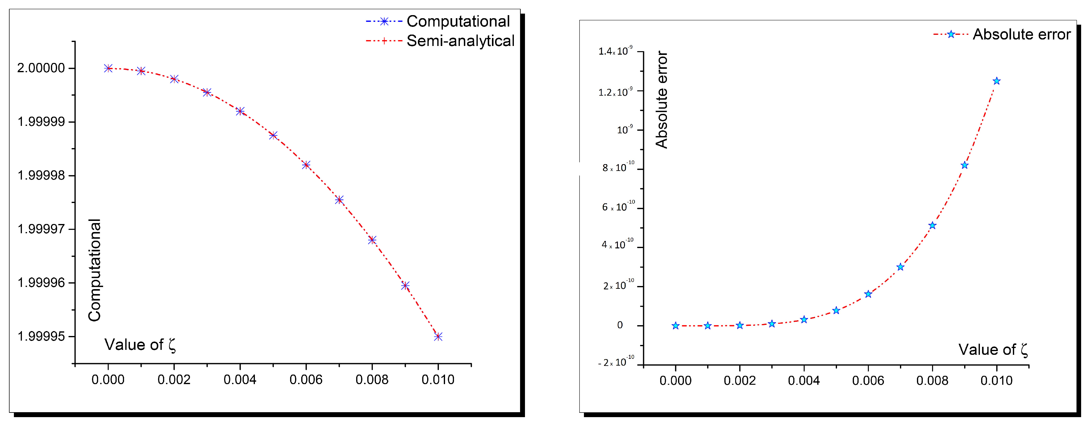
2.2. MK Method’s Solutions

Handling Equation (3) through the suggested analytical scheme’s framework allows calculation of the parameters shown above in the following forms:
Family I
a 0 = 0 , a 1 = 6 c + r 3 + 1 r 1 , a 2 = 6 c + r 3 + 1 r 1 , r 2 = c r 3 1 c ln ( a ) 2 .
Family II
a 0 = c 1 r 1 , a 1 = 6 c + r 3 1 r 1 , a 2 = 6 c + r 3 1 r 1 , r 2 = c r 3 + 1 c ln ( a ) 2 .
Consequently, the considered model’s traveling solutions are evaluated by the following forms:
B I ( ζ , t ) = 6 c + r 3 + 1 1 ± a c t + ζ 1 r 1 1 ± a c t + ζ 1 2 ,
B II ( ζ , t ) = 1 ± a c t + ζ 1 ( c + 1 ) 1 ± a c t + ζ 1 6 + 6 r 3 + 6 c r 3 + 1 r 1 1 ± a c t + ζ 1 2 .

Semi-Analytical Solutions

  • Applying the AD method for Equation (2) with the following initial and boundary conditions Y ( 0 ) = 8 e x e x + 1 2 , Y ( 0 ) = 0 gives the following solutions
    Y 0 = 2 ,
    Y 1 = 2 2 ,
    Y 2 = 4 12 ,
    Y 3 = 4 8 6 288 .
    Thus, the semi-analytical solutions of the (2 + 1)-D KP-BBM equation are given by
    Y A p p r o x . = x 6 288 + 5 x 4 24 x 2 2 + 2 + .
  • Applying the variational iteration method for Equation (1) with the following initial condition B ( ζ , 0 ) = 8 e ζ 1 e ζ 1 + 1 2 gives the following solutions:
    B 1 ( ζ , t ) = 4 cosh 2 ζ 1 2 ( ( 4 96 t ) cosh ( ζ 1 ) + 144 t + cosh ( 2 ( ζ 1 ) ) + 3 ) ( cosh ( ζ 1 ) + 1 ) 4 ,
    B 2 ( ζ , t ) = 4 cosh 2 ζ 1 2 ( ( 4 96 t ) cosh ( ζ 1 ) + 144 t + cosh ( 2 ( ζ 1 ) ) + 3 ) ( cosh ( ζ 1 ) + 1 ) 4 3 32 t × sec h 14 ζ 1 2 ( ( 48 t ( 15232 t 57 ) 70 ) cosh ( ζ 1 ) 4 ( 48 t ( 904 t 15 ) + 5 ) × cosh ( 2 ( ζ 1 ) ) + ( 48 t ( 256 t + 25 ) + 5 ) cosh ( 3 ( ζ 1 ) ) 216 t cosh ( 4 ( ζ 1 ) ) 7 ( 24 t ( 3456 t + 25 ) + 7 ) 1932 sinh ( ζ 1 ) 1128 sinh ( 2 ( ζ 1 ) ) + 78 sinh ( 3 ( ζ 1 ) ) + 132 sinh ( 4 ( ζ 1 ) ) 6 sinh ( 5 ( ζ 1 ) ) + 5 cosh ( 4 ( ζ 1 ) ) + cosh ( 5 ( ζ 1 ) ) ) .

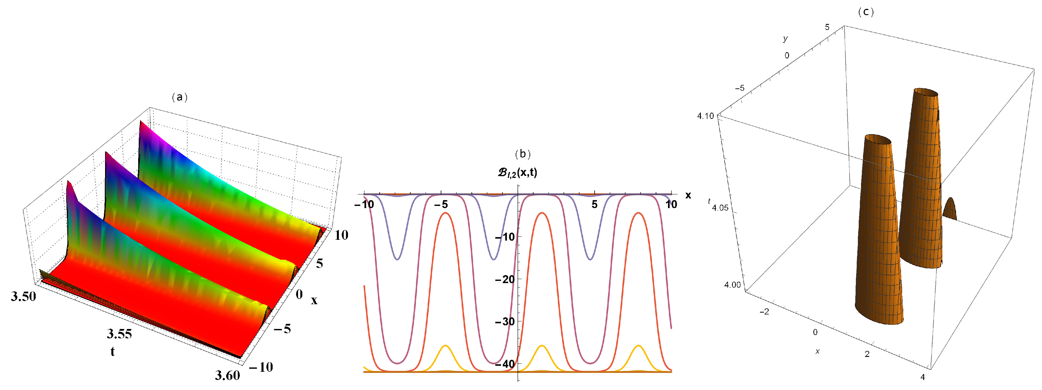
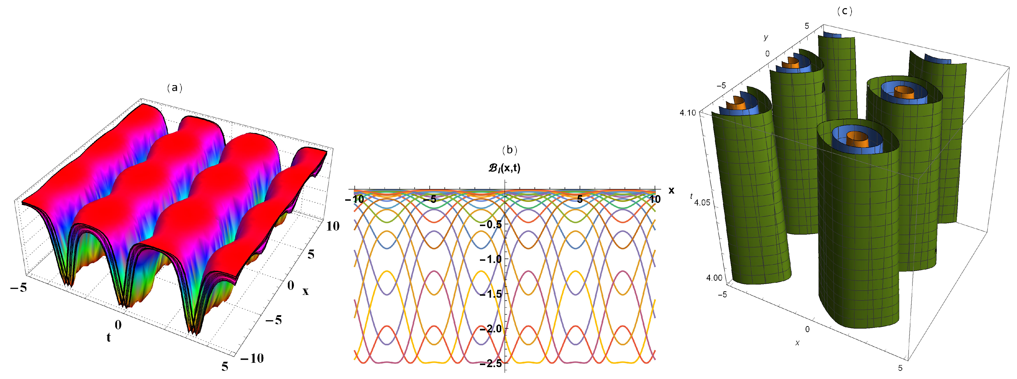
3. Interpretation of Results

In this section the interpretation of the results and the paper’s contribution are shown through comparing the obtained results with those that have been recently published for the considered model. Comparing our analytical solutions with those that have been obtained by [21,22,23] shows the novelty of our result, where all our solutions are completely different from those that have been obtained in those papers. Additionally, we explain the shown figures for more physical explanation of each of them and for demonstration of the flow’s dynamical behavior. Figure 1, Figure 2, Figure 3, Figure 4, Figure 5, Figure 6, Figure 7 and Figure 8 show breather and kink wave in two and three-dimensions and the contour plot of Equations (4), (7), (25) and (26) when [ a 1 = 4 , c = 3 , J 2 = 2 , J 3 = 7 , ϑ = 10 & a 1 = 7 , c = 5 , J 2 = 4 , J 3 = 20 , ϑ = 0 & a = e , c = 5 , r 1 = 3 , r 3 = 1 & a = e , c = 5 , r 1 = 3 , r 3 = 1 ] and the matching between the computational and semi-analytical solutions is illustrated. The paper’s main target is obtaining novel traveling wave solutions of the (2 + 1)-D KP-BBM equation then investigating their accuracy by applying two numerical schemes of the same model that show the range of matching between analytical and numerical solutions. The accuracy of each of the MDA and MK methods is explained through Table 1, Table 2, Table 3 and Table 4. Based on the shown values of computational, semi-analytical and absolute error in Table 1, Table 2, Table 3 and Table 4 the obtained solution via the MK method is more accurate than that obtained by the MDA method that is demonstrated in Figure 9.

4. Conclusions

This manuscript successfully applied four analytical and numerical techniques to the (2 + 1)-D KP-BBM equation used as a shallow water wave model. Many accurate novel traveling wave solutions were obtained. The accuracy and novelty of the obtained solutions were investigated. The traveling obtained solutions were demonstrated by 2D, 3D, and contour 3D plots. The symmetry between analytical and numerical solutions is explained through the given tables and figures.

Author Contributions

M.M.A.K. and L.A. contributed in first draft, software, and methodology, M.M.A.K., D.L. and W.L. contributed in formal analysis and investigation, and writing—review and editing. All authors have read and agreed to the published version of the manuscript.

Funding

This paper has not been funded by any outside entity.

Institutional Review Board Statement

Not applicable.

Informed Consent Statement

Not applicable.

Data Availability Statement

The data that support the findings of this study are available from the corresponding author upon reasonable request.

Acknowledgments

The author is thankful of the journal stuff and reviewer for their support and comments.

Conflicts of Interest

There is no conflict of interest.

References

  1. Gao, X.Y.; Guo, Y.J.; Shan, W.R. Bilinear forms through the binary Bell polynomials, N solitons and Bäcklund transformations of the Boussinesq–Burgers system for the shallow water waves in a lake or near an ocean beach. Commun. Theor. Phys. 2020, 72, 095002. [Google Scholar] [CrossRef]
  2. Liu, J.G.; Feng, Y.Y.; Zhang, H.Y. Exploration of the algebraic traveling wave solutions of a higher order model. Eng. Comput. 2020. [Google Scholar] [CrossRef]
  3. Pandey, A.K. The effects of surface tension on modulational instability in full-dispersion water-wave models. Eur. J. Mech. B/Fluids 2019, 77, 177–182. [Google Scholar] [CrossRef]
  4. Crompton, O.; Sytsma, A.; Thompson, S. Emulation of the Saint Venant equations enables rapid and accurate predictions of infiltration and overland flow velocity on spatially heterogeneous surfaces. Water Resour. Res. 2019, 55, 7108–7129. [Google Scholar] [CrossRef]
  5. Madhusudanan, A.; Illingworth, S.J.; Marusic, I. Coherent large-scale structures from the linearized Navier–Stokes equations. J. Fluid Mech. 2019, 873, 89–109. [Google Scholar] [CrossRef]
  6. Prakash, A.; Prakasha, D.G.; Veeresha, P. A reliable algorithm for time-fractional Navier-Stokes equations via Laplace transform. Nonlinear Eng. 2019, 8, 695–701. [Google Scholar] [CrossRef]
  7. Gazzola, F.; Sperone, G. Steady Navier–Stokes Equations in Planar Domains with Obstacle and Explicit Bounds for Unique Solvability. Arch. Ration. Mech. Anal. 2020, 238, 1283–1347. [Google Scholar] [CrossRef]
  8. Abdel-Aty, A.H.; Khater, M.M.; Baleanu, D.; Abo-Dahab, S.; Bouslimi, J.; Omri, M. Oblique explicit wave solutions of the fractional biological population (BP) and equal width (EW) models. Adv. Differ. Equ. 2020, 2020, 552. [Google Scholar] [CrossRef]
  9. Abdel-Aty, A.H.; Khater, M.M.; Baleanu, D.; Khalil, E.; Bouslimi, J.; Omri, M. Abundant distinct types of solutions for the nervous biological fractional FitzHugh–Nagumo equation via three different sorts of schemes. Adv. Differ. Equ. 2020, 2020, 476. [Google Scholar] [CrossRef]
  10. Khater, M.M.; Baleanu, D. On abundant new solutions of two fractional complex models. Adv. Differ. Equ. 2020, 2020, 268. [Google Scholar] [CrossRef]
  11. Yue, C.; Khater, M.M.; Attia, R.A.; Lu, D. The plethora of explicit solutions of the fractional KS equation through liquid–gas bubbles mix under the thermodynamic conditions via Atangana–Baleanu derivative operator. Adv. Differ. Equ. 2020, 2020, 62. [Google Scholar] [CrossRef] [Green Version]
  12. Alfalqi, S.; Khater, M.; Alzaidi, J.; Lu, D. Dynamical Behaviour of the Light Pulses through the Optical Fiber: Two Nonlinear Atangana Conformable Fractional Evolution Equations. J. Math. 2020, 2020. [Google Scholar] [CrossRef]
  13. Khater, M.; Zheng, Q.; Qin, H.; Attia, R.A. On Highly Dimensional Elastic and Nonelastic Interaction between Internal Waves in Straight and Varying Cross-Section Channels. Math. Probl. Eng. 2020, 2020. [Google Scholar] [CrossRef]
  14. Khater, M.M.; Park, C.; Lu, D. Two effective computational schemes for a prototype of an excitable system. AIP Adv. 2020, 10, 105120. [Google Scholar] [CrossRef]
  15. Abdel-Aty, A.H.; Khater, M.M.; Dutta, H.; Bouslimi, J.; Omri, M. Computational solutions of the HIV-1 infection of CD4+ T-cells fractional mathematical model that causes acquired immunodeficiency syndrome (AIDS) with the effect of antiviral drug therapy. Chaos Solitons Fractals 2020, 139, 110092. [Google Scholar] [CrossRef] [PubMed]
  16. Khater, M.; Chu, Y.M.; Attia, R.A.; Inc, M.; Lu, D. On the Analytical and Numerical Solutions in the Quantum Magnetoplasmas: The Atangana Conformable Derivative (2 + 1)-ZK Equation with Power-Law Nonlinearity. Adv. Math. Phys. 2020, 2020. [Google Scholar] [CrossRef]
  17. Khater, M.M.; Attia, R.A.; Park, C.; Lu, D. On the numerical investigation of the interaction in plasma between (high & low) frequency of (Langmuir & ion-acoustic) waves. Results Phys. 2020, 18, 103317. [Google Scholar]
  18. Nadeem, M.; Li, F.; Ahmad, H. Modified Laplace variational iteration method for solving fourth-order parabolic partial differential equation with variable coefficients. Comput. Math. Appl. 2019, 78, 2052–2062. [Google Scholar] [CrossRef]
  19. Khater, M.M.; Attia, R.A.; Abdel-Aty, A.H.; Alharbi, W.; Lu, D. Abundant analytical and numerical solutions of the fractional microbiological densities model in bacteria cell as a result of diffusion mechanisms. Chaos Solitons Fractals 2020, 136, 109824. [Google Scholar] [CrossRef]
  20. Qin, H.; Khater, M.; Attia, R.A. Inelastic Interaction and Blowup New Solutions of Nonlinear and Dispersive Long Gravity Waves. J. Funct. Spaces 2020, 2020. [Google Scholar] [CrossRef]
  21. Manafian, J.; Murad, M.A.S.; Alizadeh, A.; Jafarmadar, S. M-lump, interaction between lumps and stripe solitons solutions to the (2 + 1)-dimensional KP-BBM equation. Eur. Phys. J. Plus 2020, 135, 167. [Google Scholar] [CrossRef]
  22. Tanwar, D.V.; Wazwaz, A.M. Lie symmetries, optimal system and dynamics of exact solutions of (2 + 1)-dimensional KP-BBM equation. Phys. Scr. 2020, 95, 065220. [Google Scholar] [CrossRef]
  23. Adem, K.R.; Khalique, C.M. Exact solutions and conservation laws of a (2 + 1)-dimensional nonlinear KP-BBM equation. In Abstract and Applied Analysis; Hindawi: London, UK, 2013; Volume 2013. [Google Scholar]
  24. Kudryashov, N.A.; Loguinova, N.B. Extended simplest equation method for nonlinear differential equations. Appl. Math. Comput. 2008, 205, 396–402. [Google Scholar] [CrossRef]
  25. Bilige, S.; Chaolu, T. An extended simplest equation method and its application to several forms of the fifth-order KdV equation. Appl. Math. Comput. 2010, 216, 3146–3153. [Google Scholar] [CrossRef]
  26. Hosseini, K.; Ansari, R. New exact solutions of nonlinear conformable time-fractional Boussinesq equations using the modified Kudryashov method. Waves Random Complex Media 2017, 27, 628–636. [Google Scholar] [CrossRef]
  27. Kumar, D.; Seadawy, A.R.; Joardar, A.K. Modified Kudryashov method via new exact solutions for some conformable fractional differential equations arising in mathematical biology. Chin. J. Phys. 2018, 56, 75–85. [Google Scholar] [CrossRef]
  28. Baleanu, D.; Aydogn, S.M.; Mohammadi, H.; Rezapour, S. On modelling of epidemic childhood diseases with the Caputo-Fabrizio derivative by using the Laplace Adomian decomposition method. Alex. Eng. J. 2020, 59, 3029–3039. [Google Scholar] [CrossRef]
  29. Turkyilmazoglu, M. Accelerating the convergence of Adomian decomposition method (ADM). J. Comput. Sci. 2019, 31, 54–59. [Google Scholar] [CrossRef]
  30. Anjum, N.; He, J.H. Laplace transform: Making the variational iteration method easier. Appl. Math. Lett. 2019, 92, 134–138. [Google Scholar] [CrossRef]
Figure 1. Three-dimensional (a), two-dimensional (b) and contour 3D (c) representation of Equation (4).
Symmetry 13 01085 g001
Figure 2. Three-dimensional (a), two-dimensional (b) and contour 3D (c) representation of Equation (7).
Symmetry 13 01085 g002
Figure 3. Two-dimensional plots for analytical and semi-analytical solutions (a) and calculated absolute error between both solutions (b) that were constructed by the MDA and AD methods.
Symmetry 13 01085 g003
Figure 4. Two-dimensional plot for analytical and semi-analytical solutions (a) and two-dimensional distribution plot of the calculated absolute error between both solutions (b) that were constructed by the MDA and VI methods.
Symmetry 13 01085 g004
Figure 5. Three-dimensional (a), two-dimensional (b) and contour 3D (c) representation of Equation (25).
Symmetry 13 01085 g005
Figure 6. Three-dimensional (a), two-dimensional (b) and contour 3D (c) representation of Equation (26).
Symmetry 13 01085 g006
Figure 7. Two-dimensional plots for analytical and semi-analytical solutions (a) and calculated absolute error between both solutions (b) that were constructed by the MK and AD methods.
Symmetry 13 01085 g007
Figure 8. Two-dimensional plot for analytical and semi-analytical solutions (a) and two-dimensional distribution plot of the calculated absolute error between both solutions (b) that were constructed by the MK and VI methods.
Symmetry 13 01085 g008
Figure 9. Two-dimensional plots for the calculated absolute error through the MK & AD methods and MDA & AD methods (a), and the MK & VI methods and MDA & VI methods (b) based on the shown values in Table 1, Table 2, Table 3 and Table 4.
Symmetry 13 01085 g009
Table 1. Computational, semi-analytical, and absolute error of the (2 + 1)-D KP-BBM equation along the MDA method.
Value of ComputationalSemi-AnalyticalAbsolute Error
00.6666666670.6666666670
0.0010.6662217780.6662226668.87902 × 10 7
0.0020.6657760040.6657795523.54766 × 10 6
0.0030.6653293470.665337327.97339 × 10 6
0.0040.6648818090.6648959691.41592 × 10 5
0.0050.6644333950.6644554942.20992 × 10 5
0.0060.6639841070.6640158943.17875 × 10 5
0.0070.6635339470.6635771664.32184 × 10 5
0.0080.663082920.6631393065.63859 × 10 5
0.0090.6626310270.6627023127.12843 × 10 5
0.010.6621782730.6622661818.79078 × 10 5
Table 2. Absolute error between computational and the obtained semi-analytical through the VIM of the (2 + 1)-D KP-BBM equation with different values of t and x when y = 5 .
Value of x t = 1 t = 2 t = 3 t = 4 t = 5 t = 6 t = 7 t = 8 t = 9 t = 10
09.435 × 10 5 0.00012060.00014690.00017310.00019940.00022570.0002520.00027830.000304590.0003309
19.697 × 10 6 1.018 × 10 5 1.066 × 10 5 1.114 × 10 5 1.162 × 10 5 1.21 × 10 5 1.258 × 10 5 1.307 × 10 5 1.3546 × 10 5 1.4028 × 10 5
21.256 × 10 6 1.265 × 10 6 1.274 × 10 6 1.283 × 10 6 1.291 × 10 6 1.3 × 10 6 1.309 × 10 6 1.318 × 10 6 1.3266 × 10 6 1.3354 × 10 6
31.69 × 10 7 1.691 × 10 7 1.693 × 10 7 1.694 × 10 7 1.696 × 10 7 1.698 × 10 7 1.699 × 10 7 1.701 × 10 7 1.7026 × 10 7 1.7042 × 10 7
42.285 × 10 8 2.285 × 10 8 2.285 × 10 8 2.286 × 10 8 2.286 × 10 8 2.286 × 10 8 2.287 × 10 8 2.287 × 10 8 2.2872 × 10 8 2.2875 × 10 8
53.092 × 10 9 3.092 × 10 9 3.092 × 10 9 3.092 × 10 9 3.092 × 10 9 3.092 × 10 9 3.092 × 10 9 3.092 × 10 9 3.0922 × 10 9 3.0923 × 10 9
64.184 × 10 10 4.184 × 10 10 4.184 × 10 10 4.184 × 10 10 4.184 × 10 10 4.184 × 10 10 4.184 × 10 10 4.184 × 10 10 4.1843 × 10 10 4.1843 × 10 10
75.663 × 10 11 5.663 × 10 11 5.663 × 10 11 5.663 × 10 11 5.663 × 10 11 5.663 × 10 11 5.663 × 10 11 5.663 × 10 11 5.6627 × 10 11 5.6627 × 10 11
87.664 × 10 12 7.664 × 10 12 7.664 × 10 12 7.664 × 10 12 7.664 × 10 12 7.664 × 10 12 7.664 × 10 12 7.664 × 10 12 7.6636 × 10 12 7.6636 × 10 12
91.037 × 10 12 1.037 × 10 12 1.037 × 10 12 1.037 × 10 12 1.037 × 10 12 1.037 × 10 12 1.037 × 10 12 1.037 × 10 12 1.0372 × 10 12 1.0372 × 10 12
101.404 × 10 13 1.404 × 10 13 1.404 × 10 13 1.404 × 10 13 1.404 × 10 13 1.404 × 10 13 1.404 × 10 13 1.404 × 10 13 1.4036 × 10 13 1.4036 × 10 13
111.9 × 10 14 1.9 × 10 14 1.9 × 10 14 1.9 × 10 14 1.9 × 10 14 1.9 × 10 14 1.9 × 10 14 1.9 × 10 14 1.8996 × 10 14 1.8996 × 10 14
122.571 × 10 15 2.571 × 10 15 2.571 × 10 15 2.571 × 10 15 2.571 × 10 15 2.571 × 10 15 2.571 × 10 15 2.571 × 10 15 2.5709 × 10 15 2.5709 × 10 15
133.479 × 10 16 3.479 × 10 16 3.479 × 10 16 3.479 × 10 16 3.479 × 10 16 3.479 × 10 16 3.479 × 10 16 3.479 × 10 16 3.4793 × 10 16 3.4793 × 10 16
144.709 × 10 17 4.709 × 10 17 4.709 × 10 17 4.709 × 10 17 4.709 × 10 17 4.709 × 10 17 4.709 × 10 17 4.709 × 10 17 4.7087 × 10 17 4.7087 × 10 17
156.373 × 10 18 6.373 × 10 18 6.373 × 10 18 6.373 × 10 18 6.373 × 10 18 6.373 × 10 18 6.373 × 10 18 6.373 × 10 18 6.3725 × 10 18 6.3725 × 10 18
168.624 × 10 19 8.624 × 10 19 8.624 × 10 19 8.624 × 10 19 8.624 × 10 19 8.624 × 10 19 8.624 × 10 19 8.624 × 10 19 8.6243 × 10 19 8.6243 × 10 19
171.167 × 10 19 1.167 × 10 19 1.167 × 10 19 1.167 × 10 19 1.167 × 10 19 1.167 × 10 19 1.167 × 10 19 1.167 × 10 19 1.1672 × 10 19 1.1672 × 10 19
181.58 × 10 20 1.58 × 10 20 1.58 × 10 20 1.58 × 10 20 1.58 × 10 20 1.58 × 10 20 1.58 × 10 20 1.58 × 10 20 1.5796 × 10 20 1.5796 × 10 20
192.138 × 10 21 2.138 × 10 21 2.138 × 10 21 2.138 × 10 21 2.138 × 10 21 2.138 × 10 21 2.138 × 10 21 2.138 × 10 21 2.1377 × 10 21 2.1377 × 10 21
202.893 × 10 22 2.893 × 10 22 2.893 × 10 22 2.893 × 10 22 2.893 × 10 22 2.893 × 10 22 2.893 × 10 22 2.893 × 10 22 2.8931 × 10 22 2.8931 × 10 22
213.915 × 10 23 3.915 × 10 23 3.915 × 10 23 3.915 × 10 23 3.915 × 10 23 3.915 × 10 23 3.915 × 10 23 3.915 × 10 23 3.9154 × 10 23 3.9154 × 10 23
225.299 × 10 24 5.299 × 10 24 5.299 × 10 24 5.299 × 10 24 5.299 × 10 24 5.299 × 10 24 5.299 × 10 24 5.299 × 10 24 5.2989 × 10 24 5.2989 × 10 24
237.171 × 10 25 7.171 × 10 25 7.171 × 10 25 7.171 × 10 25 7.171 × 10 25 7.171 × 10 25 7.171 × 10 25 7.171 × 10 25 7.1713 × 10 25 7.1713 × 10 25
249.705 × 10 26 9.705 × 10 26 9.705 × 10 26 9.705 × 10 26 9.705 × 10 26 9.705 × 10 26 9.705 × 10 26 9.705 × 10 26 9.7054 × 10 26 9.7054 × 10 26
251.313 × 10 26 1.313 × 10 26 1.313 × 10 26 1.313 × 10 26 1.313 × 10 26 1.313 × 10 26 1.313 × 10 26 1.313 × 10 26 1.3135 × 10 26 1.3135 × 10 26
261.778 × 10 27 1.778 × 10 27 1.778 × 10 27 1.778 × 10 27 1.778 × 10 27 1.778 × 10 27 1.778 × 10 27 1.778 × 10 27 1.7776 × 10 27 1.7776 × 10 27
272.406 × 10 28 2.406 × 10 28 2.406 × 10 28 2.406 × 10 28 2.406 × 10 28 2.406 × 10 28 2.406 × 10 28 2.406 × 10 28 2.4057 × 10 28 2.4057 × 10 28
283.256 × 10 29 3.256 × 10 29 3.256 × 10 29 3.256 × 10 29 3.256 × 10 29 3.256 × 10 29 3.256 × 10 29 3.256 × 10 29 3.2558 × 10 29 3.2558 × 10 29
294.406 × 10 30 4.406 × 10 30 4.406 × 10 30 4.406 × 10 30 4.406 × 10 30 4.406 × 10 30 4.406 × 10 30 4.406 × 10 30 4.4062 × 10 30 4.4062 × 10 30
305.963 × 10 31 5.963 × 10 31 5.963 × 10 31 5.963 × 10 31 5.963 × 10 31 5.963 × 10 31 5.963 × 10 31 5.963 × 10 31 5.9632 × 10 31 5.9632 × 10 31
Table 3. Computational, semi-analytical, and absolute error of the (2 + 1)-D KP-BBM equation along the MK method.
Value of ComputationalSemi-AnalyticalAbsolute Error
0220
0.0011.99999951.99999951.25011 × 10 13
0.0021.9999981.9999982.0004 × 10 12
0.0031.99999551.99999551.01248 × 10 11
0.0041.9999921.9999923.20004 × 10 11
0.0051.99998751.99998757.81248 × 10 11
0.0061.9999821.9999821.62 × 10 10
0.0071.99997551.9999755013.00126 × 10 10
0.0081.9999681.9999680015.12002 × 10 10
0.0091.9999595011.9999595018.20129 × 10 10
0.011.9999500011.9999500021.25001 × 10 9
Table 4. Absolute error between computational and the obtained semi-analytical through the VIM of the (2 + 1)-D KP-BBM equation with different values of t and x when y = 5 .
Value of x t = 1 t = 2 t = 3 t = 4 t = 5 t = 6 t = 7 t = 8 t = 9 t = 10
00.12483860.2421380.25548870.06848110.41529421.29224692.65878654.61132257.2462645410.6600221
10.01869970.04021940.06256570.08374560.10176570.11463280.12035370.11693510.102383770.07470652
20.00255760.00532410.00826150.01133140.01449590.01771670.02095570.02417460.027335440.03039995
30.00034610.00070390.00107280.00145190.00184070.00223830.00264420.00305750.003477550.00390366
44.681 × 10 5 9.423 × 10 5 0.00014220.00019080.000240.00028970.000340.00039080.000442110.00049393
56.333 × 10 6 1.27 × 10 5 1.909 × 10 5 2.552 × 10 5 3.197 × 10 5 3.846 × 10 5 4.497 × 10 5 5.151 × 10 5 5.8086 × 10 5 6.4687 × 10 5
68.57 × 10 7 1.716 × 10 6 2.576 × 10 6 3.437 × 10 6 4.3 × 10 6 5.165 × 10 6 6.031 × 10 6 6.899 × 10 6 7.768 × 10 6 8.6387 × 10 6
71.16 × 10 7 2.32 × 10 7 3.482 × 10 7 4.644 × 10 7 5.806 × 10 7 6.97 × 10 7 8.134 × 10 7 9.3 × 10 7 1.0465 × 10 6 1.1632 × 10 6
81.57 × 10 8 3.139 × 10 8 4.71 × 10 8 6.28 × 10 8 7.851 × 10 8 9.423 × 10 8 1.099 × 10 7 1.257 × 10 7 1.414 × 10 7 1.5712 × 10 7
92.124 × 10 9 4.248 × 10 9 6.373 × 10 9 8.498 × 10 9 1.062 × 10 8 1.275 × 10 8 1.487 × 10 8 1.7 × 10 8 1.9124 × 10 8 2.125 × 10 8
102.875 × 10 10 5.749 × 10 10 8.624 × 10 10 1.15 × 10 9 1.437 × 10 9 1.725 × 10 9 2.012 × 10 9 2.3 × 10 9 2.5875 × 10 9 2.8751 × 10 9
113.89 × 10 11 7.781 × 10 11 1.167 × 10 10 1.556 × 10 10 1.945 × 10 10 2.334 × 10 10 2.723 × 10 10 3.112 × 10 10 3.5016 × 10 10 3.8906 × 10 10
125.265 × 10 12 1.053 × 10 11 1.58 × 10 11 2.106 × 10 11 2.633 × 10 11 3.159 × 10 11 3.686 × 10 11 4.212 × 10 11 4.7387 × 10 11 5.2652 × 10 11
137.126 × 10 13 1.425 × 10 12 2.138 × 10 12 2.85 × 10 12 3.563 × 10 12 4.275 × 10 12 4.988 × 10 12 5.7 × 10 12 6.4131 × 10 12 7.1256 × 10 12
149.643 × 10 14 1.929 × 10 13 2.893 × 10 13 3.857 × 10 13 4.822 × 10 13 5.786 × 10 13 6.75 × 10 13 7.715 × 10 13 8.6791 × 10 13 9.6434 × 10 13
151.305 × 10 14 2.61 × 10 14 3.915 × 10 14 5.22 × 10 14 6.525 × 10 14 7.831 × 10 14 9.136 × 10 14 1.044 × 10 13 1.1746 × 10 13 1.3051 × 10 13
161.766 × 10 15 3.533 × 10 15 5.299 × 10 15 7.065 × 10 15 8.831 × 10 15 1.06 × 10 14 1.236 × 10 14 1.413 × 10 14 1.5896 × 10 14 1.7663 × 10 14
172.39 × 10 16 4.781 × 10 16 7.171 × 10 16 9.561 × 10 16 1.195 × 10 15 1.434 × 10 15 1.673 × 10 15 1.912 × 10 15 2.1513 × 10 15 2.3904 × 10 15
183.235 × 10 17 6.47 × 10 17 9.705 × 10 17 1.294 × 10 16 1.618 × 10 16 1.941 × 10 16 2.265 × 10 16 2.588 × 10 16 2.9115 × 10 16 3.235 × 10 16
194.378 × 10 18 8.756 × 10 18 1.313 × 10 17 1.751 × 10 17 2.189 × 10 17 2.627 × 10 17 3.065 × 10 17 3.502 × 10 17 3.9403 × 10 17 4.3781 × 10 17
205.925 × 10 19 1.185 × 10 18 1.778 × 10 18 2.37 × 10 18 2.963 × 10 18 3.555 × 10 18 4.148 × 10 18 4.74 × 10 18 5.3326 × 10 18 5.9251 × 10 18
218.019 × 10 20 1.604 × 10 19 2.406 × 10 19 3.208 × 10 19 4.009 × 10 19 4.811 × 10 19 5.613 × 10 19 6.415 × 10 19 7.2169 × 10 19 8.0188 × 10 19
221.085 × 10 20 2.17 × 10 20 3.256 × 10 20 4.341 × 10 20 5.426 × 10 20 6.511 × 10 20 7.597 × 10 20 8.682 × 10 20 9.767 × 10 20 1.0852 × 10 19
231.469 × 10 21 2.937 × 10 21 4.406 × 10 21 5.875 × 10 21 7.343 × 10 21 8.812 × 10 21 1.028 × 10 20 1.175 × 10 20 1.3218 × 10 20 1.4687 × 10 20
241.988 × 10 22 3.975 × 10 22 5.963 × 10 22 7.951 × 10 22 9.938 × 10 22 1.193 × 10 21 1.391 × 10 21 1.59 × 10 21 1.7889 × 10 21 1.9877 × 10 21
252.69 × 10 23 5.38 × 10 23 8.07 × 10 23 1.076 × 10 22 1.345 × 10 22 1.614 × 10 22 1.883 × 10 22 2.152 × 10 22 2.421 × 10 22 2.69 × 10 22
263.64 × 10 24 7.281 × 10 24 1.092 × 10 23 1.456 × 10 23 1.82 × 10 23 2.184 × 10 23 2.548 × 10 23 2.912 × 10 23 3.2765 × 10 23 3.6405 × 10 23
274.928 × 10 25 9.855 × 10 25 1.478 × 10 24 1.971 × 10 24 2.464 × 10 24 2.956 × 10 24 3.449 × 10 24 3.942 × 10 24 4.4343 × 10 24 4.927 × 10 24
286.667 × 10 26 1.333 × 10 25 2 × 10 25 2.667 × 10 25 3.334 × 10 25 4.001 × 10 25 4.667 × 10 25 5.334 × 10 25 6.001 × 10 25 6.6678 × 10 25
299.024 × 10 27 1.805 × 10 26 2.707 × 10 26 3.61 × 10 26 4.512 × 10 26 5.414 × 10 26 6.317 × 10 26 7.219 × 10 26 8.1216 × 10 26 9.0238 × 10 26
301.221 × 10 27 2.443 × 10 27 3.664 × 10 27 4.886 × 10 27 6.106 × 10 27 7.328 × 10 27 8.549 × 10 27 9.769 × 10 27 1.0992 × 10 26 1.2213 × 10 26
Publisher’s Note: MDPI stays neutral with regard to jurisdictional claims in published maps and institutional affiliations.

