An Alternative One-Parameter Distribution for Bounded Data Modeling Generated from the Lambert Transformation

Abstract

The beta and Kumaraswamy distributions are two of the most widely used distributions for modeling bounded data. When the histogram of a certain dataset exhibits increasing or decreasing behavior, one-parameter distributions such as the power, Marshall–Olkin extended uniform and skew-uniform distributions become viable alternatives. In this article, we propose a new one-parameter distribution for modeling bounded data, the Lambert-uniform distribution. The proposal can be considered as a natural alternative to well known one-parameter distributions in the statistical literature and, in certain scenarios, a viable alternative even for the two-parameter beta and Kumaraswamy distributions. We show that the density function of the proposal tends to positive finite values at the ends of the support, a behavior that favors good performance in certain scenarios. The raw moments are derived from the moment-generating function and used to describe the skewness and kurtosis behavior. The quantile function is expressed in closed form in terms of the Lambert W function, which allows reparameterizing the distribution such that the involved parameter represents the qth quantile. Thus, for the analysis of a bounded range variable, for which a set of covariates is available, we propose a regression model that relates the qth quantile of the response to a linear predictor through a link function. The parameter estimation is carried out using the maximum likelihood method and the behavior of the estimators is evaluated through simulation experiments. Finally, three application examples are considered in order to illustrate the usefulness of the proposal.

1. Introduction

It is common to deal with data expressed as a proportion, percentage, rate or fraction in the continuous range $(0,1)$ when analyzing certain random phenomena, for example, when observing the annual replacement rate related to blue collar workers [1], the proportion of codling moth eggs that die from fumigation with methyl bromide [2] and the percentage difference in nicotine levels in users of first and new generation e-cigarette devices [3].

Two widely used probability distributions in data modeling such as those described above are the two-parameter beta (B) [4] and Kumaraswamy (K) [5] distributions. These distributions have a very flexible probability density function (pdf), presenting monotonic, unimodal and U shapes. Although these distributions are usually the first alternatives considered for modeling bounded data, it is possible to find in the statistical literature one-parameter distributions that can appropriately model datasets whose histograms show increasing or decreasing behavior. In this scenario, the power (P) distribution, which can be derived as a special case of the B and K distributions, and the Marshall–Olkin extended uniform (MOEU) [6] and skew-uniform (SU) [7] distributions, which are the result of the popular approach of adding a parameter to a baseline distribution in search of a more flexible distribution, can be considered viable alternatives.

A notable characteristic shared by these latter distributions is that the pdfs tend monotonically to finite values (functions of the parameters) at the extremes of the support, which in certain scenarios allows the extreme sample quantiles to be much more adequately modeled. However, on occasions, due to the curvature characteristics of the pdfs, the modeling of the most central quantiles may not be good, which in turn affects the quality of the fit of the extreme quantiles. Consequently, the performance of the P, MOEU and SU distributions is not good. In such a case, the B and K distributions, having two shape parameters, can properly model the most central quantiles due to the great flexibility exhibited by the pdfs in terms of curvature.

Motivated by the above, we formulate the following question as a starting point in this work: Based on the approach of adding parameters to a baseline distribution, is it possible to generate a parsimonious distribution that can perform better than the P, MOEU, SU, B and K distributions when modeling data whose histogram exhibits increasing or decreasing behavior?

To answer such question, we consider the Lambert-F distribution generator [8] defined by the cumulative distribution function (cdf) given by $G(x;\alpha )=1-[1-F\left(x\right)]{\alpha }^{F\left(x\right)}$, where $\alpha \in (0,e)$ is a shape parameter, $e\approx 2.718$ is the Euler’s number and $F\left(x\right)$ is an arbitrary baseline cdf. This generator has the particularity that the inverse function, that is, the quantile function, can be expressed in closed form in terms of the Lambert W function defined in Appendix A. If the baseline distribution $F\left(x\right)$ is symmetric, it can be verified that $\alpha$ performs as a skewness parameter, allowing asymmetric shapes for the resulting pdf (for more details, see Iriarte et al. [9]).

In this article, we introduce a new one-parameter distribution that is especially useful for modeling bounded data from a population whose pdf has a monotonic (increasing or decreasing) behavior. The proposal arises directly from the Lambert-F generator when considering a uniform (U) baseline distribution. We observe that the pdf of the proposed distribution, called the Lambert-uniform (LU) distribution, tends to finite values at the ends of the support, which in certain scenarios favors the good performance of the distribution. Consequently, the LU distribution may perform better in data modeling than the P, MOEU, SU, B and K distributions. We show that the LU distribution can be reparameterized in terms of its qth quantile. Thus, based on this result, we propose a regression model that relates the qth quantile of the response to a linear predictor through a link function. The proposed model can be considered as an alternative to quantile regression models available in the literature, such as the K quantile regression model, and performs adequately in scenarios where the histogram of the observed values of the response variable exhibits an increasing or decreasing behavior.

The article is organized as follows. In Section 2, we propose the LU distribution, derive its main structural properties, describe the skewness and kurtosis characteristics and discuss the parameter estimation under the maximum likelihood (ML) method. In Section 3, we propose the quantile regression model based on the LU distribution and discuss the estimation of the regression coefficients via the ML method. In Section 4, the behavior of the estimators is evaluated in scenarios with and without covariates. Section 5 presents three application examples illustrating the usefulness of the propose. Finally, the main conclusions are reported in Section 6.

2. Lambert-Uniform Distribution

In this section, we define the Lambert-uniform random variable and derive the density, distribution and quantile functions.

2.1. LU Random Variable

Definition 1.

A random variable X follows a Lambert-uniform distribution, with shape parameters $\alpha \in (0,e)$, denoted as $X\sim \mathrm{LU}\left(\alpha \right)$, if it can be represented as

$$\begin{array}{c}\hfill X=\left\{\begin{array}{c}{\displaystyle \frac{1}{log\left(\alpha \right)}{W}_0\left(\frac{log\left(\alpha \right)(U-1)}{\alpha }\right)+1,\mathrm{if}\alpha \in (0,1)\cup (1,e),}\hfill \\ {\displaystyle U,\mathrm{if}\alpha =1,}\hfill \end{array}\right.\end{array}$$

(1)

where $W_0(·)$ is the principal branch of the Lambert W function and U is a uniform $(0,1)$ random variable.

In Definition 1, taking into account that $W_0(·)$ is a monotonic function, it is observed that X corresponds to a one-to-one transformation of the uniform random variable. Furthermore, it is observed that the analytic expression $W_0[log\left(\alpha \right)(U-1)/\alpha ]/log\left(\alpha \right)+1$ assumes values in the interval $(0,1)$ for all $U\in (0,1)$ and $\alpha \in (0,e)$, which means that X assumes values in this same interval.

Proposition 1.

Let $X\sim \mathrm{LU}\left(\alpha \right)$. Then, the cdf of X is given by $F_X(x;\alpha )=1-\left(1-x\right){\alpha }^x$, where $x\in (0,1)$ and $\alpha \in (0,e)$.

Proof. 

From Equation (1), for $\alpha \ne 1$, we have that

$$\begin{array}{c}\hfill F_X(x;\alpha )=P(X\le x)=P\left(W_0\left[\frac{log\left(\alpha \right)(U-1)}{\alpha }\right]\le log\left(\alpha \right)\left(x-1\right)\right).\end{array}$$

Then, by definition of the Lambert W function, it follows that

$$\begin{array}{c}\hfill P(X\le x)=P\left(\frac{log\left(\alpha \right)(U-1)}{\alpha }\le log\left(\alpha \right)\left(x-1\right){\alpha }^{x-1}\right)=P\left(U\le 1-\left(1-x\right){\alpha }^x\right),\end{array}$$

and the result is obtained taking into account that $P(U\le u)=u$, since $U\sim \mathrm{uniform}(0,1)$. Finally, note that the expression obtained is also valid for $\alpha =1$, once $F_X(x;1)=x$. □

The pdf of X can be obtained in a straightforward way from Proposition 1.

Corollary 1.

Let $X\sim \mathrm{LU}\left(\alpha \right)$. Then, the pdf of X is given by $f_X(x;\alpha )={\alpha }^x\left[1-log\left(\alpha \right)\left(1-x\right)\right]$.

Consistent with Definition 1, it is observed that the cdf and the pdf of the LU distribution reduce to the cdf and the pdf of the U distribution when $\alpha =1$. Therefore, the LU distribution can be understood as an extension with one extra parameter of the U distribution.

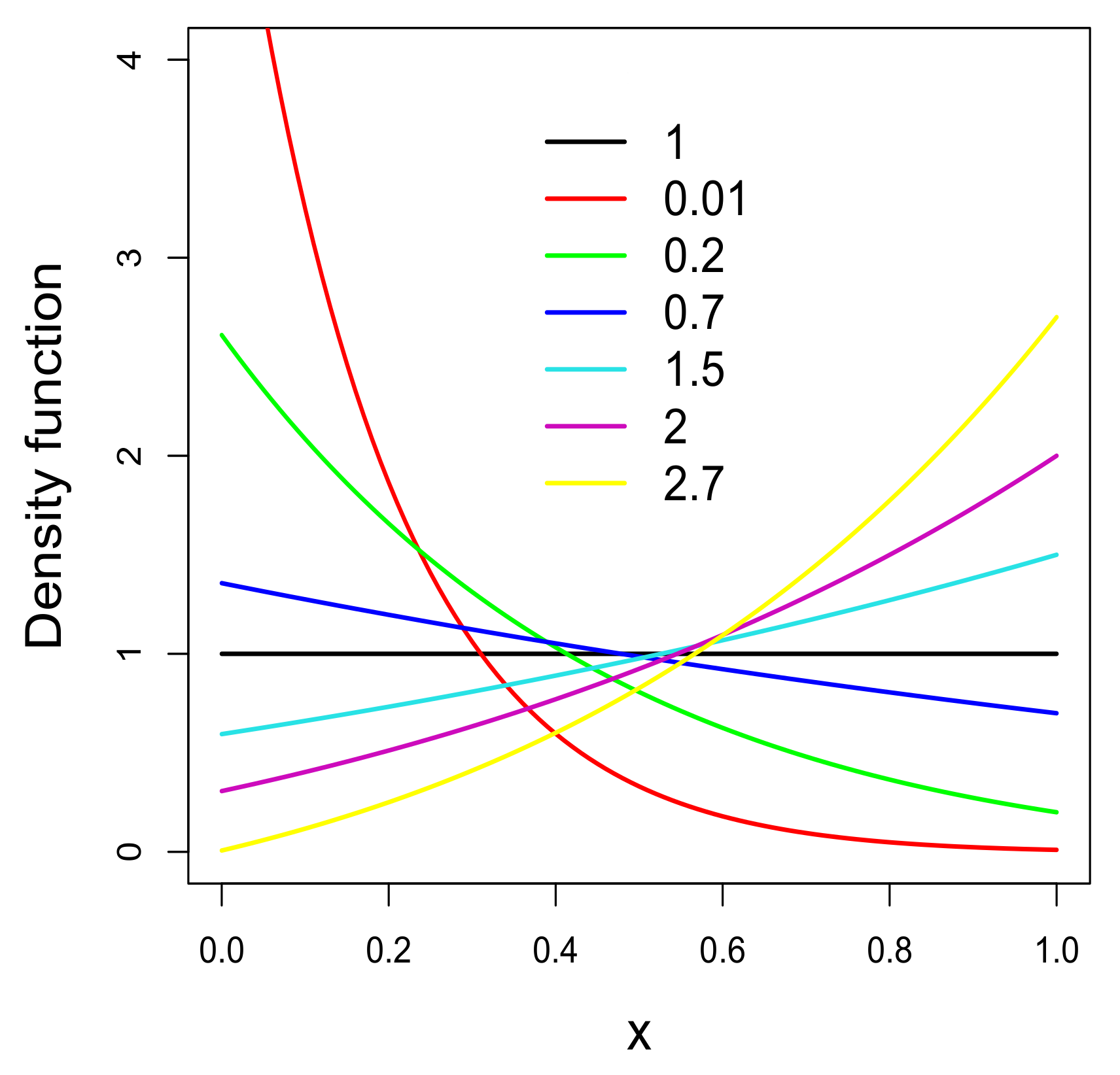
The analytical description of the shapes for the LU pdf is simple and leads to establish that: (i) ${lim}_{x\to 0^{+}}{f}_X(x;\alpha )=1-log\left(\alpha \right)$ and ${lim}_{x\to 1^{-}}{f}_X(x;\alpha )=\alpha$. (ii) $f_X(x;\alpha )$ is a constant function when $\alpha =1$, a decreasing monotonic function when $\alpha \in (0,1)$ and an increasing monotonic function when $\alpha \in (1,e)$. Property (i) shows that the pdf of the LU distribution converges to finite values (greater than 0) as x tends to the extreme values, 0 and 1, of the support. From Property (ii), it follows that the LU distribution is appropriate to fit bounded data whose relative frequency shows increasing or decreasing behavior. Figure 1 shows some pdf curves of the LU distribution for different values of the parameter $\alpha$. Note that the behavior of the pdf curves is consistent with what is established above. In addition, note that the curvature of the pdf varies depending on its behavior at the ends of the support. Thus, the behavior of the LU pdf is similar to that of the P, MOEU and SU pdfs.

Note that, due to the behavior of the pdf at the ends of the support, the LU distribution may more adequately fit the extreme sample quantiles than a distribution whose pdf tends to ∞ and 0 at the ends of the support. In Section 5, we see that the LU distribution may perform better in fitting data than the P, MOEU and SU distributions, even better than the two-parameter B and K distributions whose pdfs (in the monotonic case) tend to ∞ and 0 at the ends of the support.

Considering steps very similar to those of the proof of Proposition 1, the quantile function (qf) of the LU distribution can be easily derived by inverting the cdf given in Proposition 1. The resulting analytical expression for this function, for $u\in (0,1)$, is given by

$$\begin{array}{c}\hfill Q_X(u;\alpha )=\left\{\begin{array}{c}{\displaystyle \frac{1}{log\left(\alpha \right)}{W}_0\left(\frac{log\left(\alpha \right)(u-1)}{\alpha }\right)+1,\mathrm{if}\alpha \in (0,1)\cup (1,e),}\hfill \\ {\displaystyle u,\mathrm{if}\alpha =1.}\hfill \end{array}\right.\end{array}$$

(2)

Since the Lambert W function is implemented in different statistical software, Equation (2) can be easily computed.

As a final consideration of this section, we highlight that the linear transformation $a+bX$, where $X\sim \mathrm{LU}\left(\alpha \right)$, $a\in \mathbb{R}$ and $b>0$, follows a LU distribution on the continuous range $(a,a+b)$. Therefore, the LU distribution can be easily used to fit bounded data to any real range.

2.2. Related Distributions

It is well known that some distributions such as the exponential, Rayleigh and power, among others, can be derived as a transformation of a uniform random variable. Considering these transformations on a LU random variable, we derive the following distributions: (1) Let $Y=-\lambda log(1-X)$, where $X\sim \mathrm{LU}\left(\alpha \right)$ and $\lambda >0$. Then, Y follows the Lambert-exponential distribution, see Iriarte et al. [8]. (2) Let $Y=\sigma \sqrt{-log(1-X)}$, where $X\sim \mathrm{LU}\left(\alpha \right)$ and $\sigma >0$. Then, Y follows the Lambert–Rayleigh distribution (see Iriarte et al. [8]). (3) Let $Y=X^{1/\delta }$, where $X\sim \mathrm{LU}\left(\alpha \right)$ and $\delta >0$. Then, the distribution of Y is a two-parameter distribution that reduces to the P distribution when $\alpha =1$. In this case, the pdf of Y is given by $f_Y(y;\delta ,\alpha )=\delta y^{\delta -1}{\alpha }^{y^{\delta }}\left[1-log\left(\alpha \right)(1-y^{\delta })\right]$, where $y\in (0,1)$. Thus, we refer to this distribution as the Lambert-power distribution.

Other distributions of the literature can be derived under consideration of appropriate transformations of LU random variables. Illustratively, we consider in this section only the three transformations described above.

2.3. Skewness and Kurtosis

In the following, a description of the skewness and kurtosis characteristics of the LU distribution is made by analyzing Fisher’s asymmetry and kurtosis coefficients. For this, the moment generating function is first calculated.

Proposition 2.

Let $X\sim \mathrm{LU}\left(\alpha \right)$. Then, in the case $\alpha =1$, the moment generating function of X is given by $M_X\left(t\right)=(e^t-1)/t$. In the case $\alpha \in (0,1)\cup (1,e)$, the moment generating function is given by $M_X\left(t\right)=\{{log}^2\left(\alpha \right)-[1-log\left(\alpha \right)]t+\alpha t{e}^t\}{[t+log\left(\alpha \right)]}^{-2}$.

Proof. 

In the case $\alpha =1$, the distribution LU reduces to standard U distribution, thus $M_x\left(t\right)=\mathbb{E}\left(e^{tX}\right)=(e^t-1)/t$. In the case $\alpha \in (0,1)\cup (1,e)$, we observe that

$$\begin{array}{c}\hfill \mathbb{E}\left(e^{tX}\right)=\frac{[1-log(\alpha \left)\right][\alpha exp(t)-1]}{t+log\left(\alpha \right)}+log\left(\alpha \right){\int }_0^{1}xexp\left\{x[t+log\left(\alpha \right)]\right\}dx,\end{array}$$

and the result is obtained considering the usual method of integration by parts and an appropriate algebra. □

Corollary 2.

Let $X\sim \mathrm{LU}\left(\alpha \right)$. Then, in the case $\alpha =1$, the first four raw moments of X are $\mathbb{E}\left(X\right)=1/2$, $\mathbb{E}\left(X^2\right)=1/3$, $\mathbb{E}\left(X^3\right)=1/4$ and $\mathbb{E}\left(X^4\right)=1/5$. In the case $\alpha \in (0,1)\cup (1,e)$, for $\delta =log\left(\alpha \right)$, the first four raw moments are given by

$$\begin{array}{c}\hfill \mathbb{E}\left(X\right)=\frac{\alpha -1-\delta }{{\delta }^2},\mathbb{E}\left(X^3\right)=\frac{3[\alpha {\delta }^2-2\delta (2\alpha +1)-6(1-\alpha )]}{{\delta }^4},\\ \hfill \mathbb{E}\left(X^2\right)=\frac{2\left[\right(\alpha +1)\delta +2(1-\alpha \left)\right]}{{\delta }^3},\mathbb{E}\left(X^4\right)=\frac{4[\alpha {\delta }^2(\delta -6)+6\delta (3\alpha +1)+24(1-\alpha )]}{{\delta }^5}.\end{array}$$

Corollary 3.

Let $X\sim \mathrm{LU}\left(\alpha \right)$. Then, in the case $\alpha =1$, the skewness (${\gamma }_1\left(\alpha \right)$) and kurtosis (${\gamma }_2\left(\alpha \right)$) coefficients assume the values 0 and 9/5, respectively. In the case $\alpha \in (0,1)\cup (1,e)$, the coefficients are given by

$$\begin{array}{c}\hfill {\gamma }_1\left(\alpha \right)=\frac{{\mu }_3-3{\mu }_1{\mu }_2+2{\mu }_1^3}{{({\mu }_2-{\mu }_1)}^{3/2}}\mathrm{and}{\gamma }_2\left(\alpha \right)=\frac{{\mu }_4-4{\mu }_1{\mu }_3+6{\mu }_1^2{\mu }_2-3{\mu }_1^4}{{({\mu }_2-{\mu }_1)}^2}.\end{array}$$

where ${\mu }_r=\mathbb{E}\left(X^r\right)$, with $r=1,2,3,4$, are as in Corollary 2.

The skewness and kurtosis ranges for the LU distribution are $(3e-6e^2+2e^3-4)\left[{(2+2e-e^2)}^{-3/2}\right]<{\gamma }_1\left(\alpha \right)<2$ and $9/5<{\gamma }_2\left(\alpha \right)<9$.

Figure 2 presents plots of the coefficients given in Corollary 3. The figure shows that the LU distribution is symmetric only in the case $\alpha =1$, has positive skewness when $\alpha \in (0,1)$ and has negative skewness when $\alpha \in (1,e)$. Furthermore, it is observed that the LU distribution can model kurtosis levels higher than the kurtosis level of the U distribution.

2.4. ML Estimation

For a random sample $X_1,\dots ,X_n$, such that $X_i\sim \mathrm{LU}\left(\alpha \right)$, with $i=1,\dots ,n$, the log-likelihood function is given by

$$\begin{array}{c}\hfill \ell \left(\alpha \right)=log\prod _{i=1}^n{f}_X(x_i;\alpha )=log\left(\alpha \right)\sum _{i=1}^n{x}_i+\sum _{i=1}^{n}log[1-log\left(\alpha \right)(1-x_i)],\end{array}$$

(3)

where $\overline{x}$ is the mean of the observed sample. Thus, the score function is given by

$$\begin{array}{c}\hfill \mathcal{U}\left(\alpha \right)=\frac{\partial \ell \left(\alpha \right)}{\partial \alpha }=\frac{1}{\alpha }\sum _{i=1}^n{x}_i-\frac{1}{\alpha }\sum _{i=1}^n\frac{1-x_i}{1-log\left(\alpha \right)(1-x_i)}.\end{array}$$

(4)

From Equation (4), it is observed that the ML estimator for $\alpha$ cannot be explicitly expressed. Therefore, the ML estimate of $\alpha$ must be obtained by solving the equation $\mathcal{U}\left(\alpha \right)=0$ by numerical procedures. The uniroot.all function available in the rootSolve package of the R programming language [10] is a good option to tackle this task.

Since the ML estimator of $\alpha$ does not have a closed form, a good alternative to obtain the ML estimate is to solve the optimization problem ${max}_{\alpha }\ell \left(\alpha \right)$, subject to $\alpha \in (0,e)$. To solve this problem, we use the optim function in the R programming language under the L-BFGS-B algorithm. This algorithm requires the specification of a value in the range of $\alpha$ to initialize the iterative process. Through simulation experiments, we observe that the initial value ${\alpha }_0=1$ is a good initial value.

The second partial derivative of the $\ell \left(\alpha \right)$ function, with respect to $\alpha$, is given by

$$\begin{array}{c}\hfill \frac{{\partial }^2\ell \left(\alpha \right)}{\partial {\alpha }^2}=-\frac{1}{{\alpha }^2}\sum _{i=1}^n{x}_i+\frac{1}{{\alpha }^2}\sum _{i=1}^n\frac{1-x_i}{1-log\left(\alpha \right)(1-x_i)}-\frac{1}{{\alpha }^2}\sum _{i=1}^n{\left(\frac{1-x_i}{1-log\left(\alpha \right)(1-x_i)}\right)}^2.\end{array}$$

Thus, under regularity conditions, we observe that the Fisher information is given by

$$\begin{array}{c}\hfill \mathcal{I}\left(\alpha \right)=-\mathbb{E}\left(\frac{{\partial }^2\ell \left(\alpha \right)}{\partial {\alpha }^2}\right)=\frac{n}{\alpha }{\int }_0^1\frac{u^2}{{\alpha }^u[1-log\left(\alpha \right)u]}du.\end{array}$$

(5)

The integral in Equation (5) can be calculated by numerical integration, for example, the integrate function of the R programming language can be used. Then, under regularity conditions, the asymptotic distribution of $(\widehat{\alpha }-\alpha )$ is $N(0,{\mathcal{I}}^{-1}\left(\alpha \right))$. Thus, the asymptotic standard error of $\widehat{\alpha }$ is given by $1/\sqrt{\mathcal{I}\left(\widehat{\alpha }\right)}$ and the asymptotic $100(1-\gamma )\%$ confidence interval for $\widehat{\alpha }$ is given by $\widehat{\alpha }\pm z_{\gamma /2}/\sqrt{\mathcal{I}\left(\widehat{\alpha }\right)}$, where $\gamma /2$ is the $\gamma /2$ upper quantile of the standard normal distribution.

3. Quantile Regression Model

In statistical modeling, the regression technique is used to quantify the relationship between the dependent variable (response) and one or more independent variables (covariates). In the case in which the interest lies in quantifying the effect on the conditional mean response, given the covariates, the classical least squares regression model and the generalized linear models are especially valued. These models have been shown to be very useful when analyzing data in various areas of knowledge. However, there are scenarios where it is equally or even more important to quantify the effect on some other measure such as the conditional median or some extreme conditional quantile of the response (see, e.g., [11,12]). In this scenario, a quantile regression model is appropriate because it allows quantifying the effect of the covariates on any conditional quantile of the response.

In the case of a continuous bounded range response, for example bounded to the range $(0,1)$, it is possible to use the well-known beta regression model (among others) to quantify the effect of the covariates on the mean response (see [13]). Attractive alternatives to the beta regression model can be found in the literature (see, e.g., [14]). On the other hand, from a quick review of the literature, we found the K [15] and arc-secant-hyperbolic-normal (ASHN) [16] regression models among the proposals for modeling the conditional quantiles of the response. In these last two models, we emphasize that the regression depends on a shape parameter that provides great flexibility and that must be estimated together with the regression coefficients.

A very good description of regression models for bounded response variables can be found in the work of Bayes et al. [17], who proposed a mixed quantile regression model for bounded response variables.

In what follows, we propose a quantile regression model formulated from a reparameterized version of the LU distribution proposed in Section 2.1. In this model, unlike the K and ASHN models, only the regression coefficients must be estimated. This is because it is formulated from a distribution with a single shape parameter that is linked to the linear predictor through an appropriate link function. We highlight that the performance of the proposed model is appropriate in scenarios where the histogram of the observed values of the response variable exhibits a decreasing or increasing behavior.

3.1. The LU Model

In Corollary 2, it can be seen that the mean of the LU distribution has a closed form. However, despite this, we observe that the shape parameter $\alpha$ cannot be expressed explicitly as a function of the mean, which is a major drawback to formulate a regression model to quantify the effect of the covariates on the mean response. On the other hand, we observe that $\alpha$ can be explicitly expressed as a function of the qth quantile, which allows reparameterizing the LU distribution in terms of its qth quantile and, consequently, formulate a quantile regression model in a simple way.

Denoting by $\eta$ the qth quantile of the LU distribution, from Equation (2), we obtain that $\alpha ={[(1-q)/(1-\eta )]}^{1/\eta }$. Thus, the LU distribution can be easily reparameterized in terms of the qth quantile, obtaining (for $q\in (0,1)$ is known) the pdf given by

$$f_X(x;\eta )={\left(\frac{1-q}{1-\eta }\right)}^{\frac{x}{\eta }}\left[1-\frac{1}{\eta }log\left(\frac{1-q}{1-\eta }\right)(1-x)\right],x,\eta \in (0,1).$$

(6)

Let $X_1,\dots ,X_n$ be n random variables and denote by $x_1,\dots ,x_n$ the observed values. Assume that each $X_i$ has pdf $f_{X_i}(x;{\eta }_i)$ given in Equation (6). The LU quantile regression model is defined by establishing that the qth quantile ${\eta }_i$ of $X_i$ satisfies the functional relationship $g\left({\eta }_i\right)=w_i^t\beta$, $i=1,\dots ,n$, where $w_i={(1,w_{i1},\dots ,w_{i(k-1)})}^t$ is the vector of covariates associated to the response $x_i$, $\beta ={({\beta }_0,{\beta }_1,\dots ,{\beta }_{(k-1)})}^t$ is a k-dimensional vector of unknown regression coefficients and $g(·)$ is a strictly increasing and twice differentiable function that maps $(0,1)$ into $\mathbb{R}$ (link function). For instance, the most useful well-known link functions are the logit, log-log and probit functions.

3.2. ML Estimation

From Equation (6), the log-likelihood function is given by

$$\begin{array}{c}\hfill \ell \left(\beta \right)=log(1-q)\sum _{i=1}^n\frac{x_i}{{\eta }_i}-\sum _{i=1}^n\frac{(1-{\eta }_i)x_i}{{\eta }_i}+\sum _{i=1}^{n}log\left[1-\frac{1}{{\eta }_i}log\left(\frac{1-q}{1-{\eta }_i}\right)(1-x_i)\right],\end{array}$$

(7)

and the score functions are given by

$$\begin{array}{ccc}\hfill \frac{\partial \ell \left(\beta \right)}{\partial {\beta }_r}& =& -log(1-q)\sum _{i=1}^n\frac{x_i{\eta }_{i,r}}{{\eta }_i^2}+\sum _{i=1}^n\frac{x_{i}log(1-{\eta }_i){\eta }_{i,r}}{{\eta }_i^2}+\sum _{i=1}^n\frac{x_i{\eta }_{i,r}}{{\eta }_i(1-{\eta }_i)}\hfill \\ \hfill & & +\sum _{i=1}^n\frac{log\left(\frac{1-q}{1-{\eta }_i}\right)(1-x_i){\eta }_{i,r}}{{\eta }_i^2\left[1-\frac{1}{{\eta }_i}log\left(\frac{1-q}{1-{\eta }_i}\right)(1-x_i)\right]}-\sum _{i=1}^n\frac{(1-x_i){\eta }_{i,r}}{(1-{\eta }_i)\left[1-\frac{1}{{\eta }_i}log\left(\frac{1-q}{1-{\eta }_i}\right)(1-x_i)\right]},\hfill \end{array}$$

(8)

where ${\eta }_{i,r}=\partial {\eta }_i/\partial {\beta }_r$, ${\eta }_i=g^{-1}\left(w_i^t\beta \right)$, with $r=0,1,\dots ,k-1$. Note that ${\eta }_{i,r}$ depends on the link function. For example, if the logit link is considered, that is, $g\left(u\right)=log(u/(1-u\left)\right)$, for $u\in (0,1)$, then ${\eta }_{ir}={\eta }_i(1-{\eta }_i)w_{ir}$, where ${\eta }_i=exp\left(w_i^t\beta \right)/[1+exp\left(w_i^t\beta \right)]$, $w_{i0}=1$, with $i=1,2,\dots ,n$, $r=0,1,\dots ,k-1$.

We observe from Equation (7) that the ML estimators for the coefficients $\beta$s cannot be expressed in closed form. Thus, the ML estimates must be obtained by solving the system of score equations using numerical procedures. In the R programming language, the multirrot function of the rootSolve package is a good alternative to solve this system of equations.

In this case, since the ML estimators do not have a closed form, a good alternative to obtain ML estimates is to solve the following optimization problem ${max}_{\beta }\ell \left(\beta \right)$, $\mathrm{subject}\mathrm{to}{\beta }_r\in \mathbb{R}$, $r=0,1,\dots ,k-1$, where $\ell \left(\beta \right)$ is given in Equation (7). We solved this problem using the function optim of the R programming language and, specifically, the BFGS algorithm was applied.

Under regularity conditions, the asymptotic distribution of $({\widehat{\beta }}_{\mathrm{ML}}-\beta )$ is $N_k(0,K{\left(\beta \right)}^{-1})$, where $K\left(\beta \right)$ is the expected information matrix. Since the function $\ell \left(\beta \right)$ is not simple, it is not easy to obtain the analytical expression of this matrix. However, we obtain an approximation from the observed information matrix, whose elements are computed as minus the second partial derivatives of the log-likelihood function with respect to all the parameters (evaluated at the ML estimates). Thus, the observed information matrix is given by

$$\begin{array}{c}\hfill \begin{array}{cc}\hfill I\left(\beta \right)=& \left(\begin{array}{cccc}{\epsilon }_{{\beta }_0{\beta }_0}& {\epsilon }_{{\beta }_0{\beta }_1}& \dots & {\epsilon }_{{\beta }_0{\beta }_{k-1}}\\ {\epsilon }_{{\beta }_0{\beta }_1}& {\epsilon }_{{\beta }_1{\beta }_1}& \dots & {\epsilon }_{{\beta }_1{\beta }_{k-1}}\\ ⋮& ⋮& \ddots & ⋮\\ {\epsilon }_{{\beta }_0{\beta }_{k-1}}& {\epsilon }_{{\beta }_1{\beta }_{k-1}}& \dots & {\epsilon }_{{\beta }_{k-1}{\beta }_{k-1}}\end{array}\right),\hfill \\ \hfill {\epsilon }_{{\beta }_r{\beta }_p}=& -\frac{{\partial }^2\ell \left(\beta \right)}{\partial {\beta }_r{\beta }_p}{|}_{\beta ={\widehat{\beta }}_{\mathrm{ML}}},r,p=0,1\dots ,k-1,\hfill \end{array}\end{array}$$

where the second derivatives are presented in Appendix C.

4. Simulation Studies

In this section, we initially carry out a simulation study to evaluate the behavior of the ML estimators of the shape parameter of the LU distribution. Subsequently, we carried out a second simulation study to evaluate the behavior of the ML estimators for the coefficients of the LU quantile regression model.

4.1. First Simulation Study

In this study, 1000 random samples from the LU distribution were simulated considering the sample sizes $n=10,20,\dots ,1000$, respectively, in the scenarios $\alpha =0.5$ and $\alpha =1.5$. The samples were generated using the qf given in Equation (2). The LambertW package [18] available in the R programming language was used to compute the principal branch of the Lambert W function. The estimates were obtained by maximizing the log-likelihood function under the considerations of Section 2.4.

Figure 3 shows the average estimate (AE), the empirical standard deviation (SD) and the roots of the mean squared error (RMSE) for each of the 1000 estimates obtained for each scenario and sample size considered. In addition, the average of asymptotic standard errors (SE) and the coverage probability (CP) of the 95% asymptotic confidence intervals are also reported. In the figures, it is observed that the AEs tend to be close to the true values of $\alpha$ as the sample size increases. The SDs, RMSEs and SEs are close and decrease to zero as the sample size increases, as expected in standard asymptotic theory. It is also observed that the CPs converge to the nominal values as the sample size increases.

Note that the decreasing patterns observed in the left panels of the figure suggest an overestimation of $\alpha$ when the sample size is small. As complementary information, the AEs obtained in sample sizes less than 100 can be consulted in Appendix B.

4.2. Second Simulation Study

In this study, we simulated 1000 random samples (considering the sample sizes $n=10,20,\dots ,$ 1000, respectively) from the reparameterized LU distribution, given in Equation (6), where the shape parameter is linked via the logit function with three covariates. The samples were generated as follows:

• Definition of covariates: Generate $w_1={(w_{11},\dots ,w_{1n})}^t$, $w_2={(w_{21},\dots ,w_{2n})}^t$ and $w_3={(w_{31},\dots ,w_{3n})}^t$, where $(w_{1j},w_{2j})$ follows a bivariate normal distribution with parameters ${\mu }_1={\mu }_2=0$, ${\sigma }_1={\sigma }_2=1$ and $\rho =0.7$, with $j=1,\dots ,n$ and $w_3$ is a binary variable with probability of success depending on the variable $w_1$ through the logistic function, that is, $w_{3j}\sim \mathrm{Bernoulli}\left(p_j\right)$, where $p_j=1/[1+exp(-w_{1j})]$ $j=1,\dots ,n$.
• Definition of scenarios: We considered two scenarios, A and B, where in both we picked ${\beta }_0=-2$, ${\beta }_1=0.1$, ${\beta }_2=0.5$ and ${\beta }_3=-2.5$. Regarding the choices for q, we chose the values 0.25 for Scenario A and 0.75 for Scenario B.
• Simulate the response variable: Generate ${(u_1,\dots ,u_n)}^t$, $u_j\sim \mathrm{uniform}(0,1)$, $j=1,\dots ,n$, and calculate

  $$\begin{array}{c}\hfill x_j=\frac{{\eta }_j}{log\left(\frac{1-q}{1-{\eta }_j}\right)}{W}_0\left[log\left(\frac{1-q}{1-{\eta }_j}\right)\frac{u_j-1}{{\eta }_j}{\left(\frac{1-{\eta }_j}{1-q}\right)}^{1/{\eta }_j}\right]+1,j=1,\dots ,n,\end{array}$$

  where ${\eta }_j=exp\left(w^t\beta \right)/[1+exp\left(w^t\beta \right)]$, such that $w^t\beta ={\beta }_0+{\beta }_1{w}_{1j}+{\beta }_2{w}_{2j}+{\beta }_3{w}_{3j}$, with $j=1,\dots ,n$.

In both scenarios, under the different sample sizes, it is possible to verify that the histogram of the simulated values has a decreasing behavior.

For each simulated sample, we calculated the ML estimates for the coefficients $\beta$s under the considerations of Section 3.2. Figure 4 and Figure 5 show the AEs, SDs, SEs and RMSEs for the estimates obtained in each scenario and sample size considered. In Figure 6, the CPs of the 95% asymptotic confidence intervals are reported. Similar to the results obtained in the first simulation study, in the figures, it is observed that the AEs tend to be close to the true values of the coefficients $\beta$s as the sample size increases. The SDs, RMSEs and SEs are close and decrease to zero as the sample size increases, as expected in standard asymptotic theory. It is observed that the CPs converge to the nominal values as the sample size increases.

Note that the increasing and decreasing patterns exhibited in the top panels of Figure 4 and Figure 5 suggest an underestimation and overestimation, respectively, of the individual effect of the covariates on the 0.25th and 0.75th quantiles of the response when the sample size is small. Complementarily, the AEs of the $\beta$s obtained in sample sizes smaller than 100 can be consulted in Appendix B.

When comparing the upper right panels of the figures, a different behavior pattern is observed for the AEs of ${\beta }_3$. Therefore, the effect of the covariate $w_3$ on the 0.25th quantile of the response can be underestimated when the sample size is small, while the effect on the 0.75th quantile can be overestimated.

5. Data Analysis

In this section, three application examples are presented in order to illustrate the usefulness of the LU distribution and the LU quantile regression model. In the first, we compare the performance of the LU, P, MOEU, SU, B and P distributions in the fitting of 1000 samples generated from an LU population. Here, we highlight the virtues of the LU distribution over the aforementioned distributions, leaving open the existence of a possible real-world setting where the distributions show such performance. In the second example, we compare the performance of the LU, P, MOEU, SU, B and P distributions in fitting a real dataset. In the third example, based on a real data frame, and in order to quantify the effect of the covariates on the 0.25th, 0.5th and 0.75th quantiles of the response, we compare the performance of the LU quantile regression model with the performance of other models such as ASHN [16] and K [15] quantile regression models. In all three models, the logit function is considered to relate the qth quantile of the response to the linear predictor. The pdfs of the ASHN and K distributions are given, respectively, by

$$\begin{array}{c}\hfill f(x;\alpha ,\eta )=\frac{2\alpha {\mathsf{\Phi }}^{-1}\left(q_{\alpha }\right)}{A\left(\eta \right)x\sqrt{1-x^2}}\varphi \left(\frac{{\mathsf{\Phi }}^{-1}\left(q_{\alpha }\right)A\left(x\right)}{A\left(\eta \right)}\right){\left[2-2\mathsf{\Phi }\left(\frac{{\mathsf{\Phi }}^{-1}\left(q_{\alpha }\right)A\left(x\right)}{A\left(\eta \right)}\right)\right]}^{\alpha -1},\end{array}$$

where $x\in (0,1)$, $q_{\alpha }=1-\left(q^{1/\alpha }\right)/2$, $A\left(z\right)=log[(1+\sqrt{1-z^2})/z]$ is the hyperbolic arcsecant function, $\alpha >0$ is a shape parameter, $\eta \in (0,1)$ is a quantile parameter and $q\in (0,1)$ is known, and

$$\begin{array}{c}\hfill f(x;\beta ,\eta )=\frac{\beta log(1-q)}{log(1-{\eta }^{\beta })}{x}^{\beta -1}{(1-x^{\beta })}^{log(1-q)/log(1-{\eta }^{\beta })-1},x\in (0,1),\end{array}$$

where $\beta >0$ is a shape parameter, $\eta \in (0,1)$ is a quantile parameter and $q\in (0,1)$ is known.

The regression framework for bounded responses based on the K and ASHN distributions is very similar to the regression framework based on the LU distribution presented in Section 3.1. However, the main difference with LU regression is that it depends on a shape parameter that gives great flexibility to the modeling.

In all three examples, the parameters are estimated by maximizing the corresponding likelihood functions with the optim function in the R programming language. We compared the performance of the models by contrasting the maximum value of the log-likelihood function (ℓ) and contrasting the values associated with the Akaike Information Criterion (AIC) [19] and the Bayesian Information Criterion (BIC) [20]. In general, the best model can be chosen as the one that shows the highest ℓ value and the lowest AIC, CAIC and BIC values. In addition, we consider the usual Anderson–Darling (AD) and Cramer–von Mises (CvM) goodness-of-fit tests to assess the quality of the fits in the first and second examples. In the third example, we use these tests to assess the overall quality of fit of the regression models, by testing the hypothesis that the randomize residuals [21] follow the standard normal distribution. These residuals follow a standard normal distribution when the overall quality of fit is appropriate. We use the ad.test and cvm.test functions available in the goftest [22] package in the R programming language to calculate the statistics and p-values of these tests.

5.1. Data from an LU Population

In this example, we generate 1000 random sample of size 300 from an LU population with parameter $\alpha =0.01$. The chosen value for $\alpha$ is associated with a decreasing pdf that converges to the values 5.605 and 0.01 at the ends of the support.

Based on the AD and CvM goodness of fit tests, considering a significance level of 5%, we calculate the proportion of samples where the LU, P, MOEU, SU, B and K distributions fit the data appropriately. We call this the non-rejection rate. Additionally, we calculate the proportion of samples where each distribution presents the lowest AIC and BIC values, that is, the proportion of samples where each distribution exhibits the best performance. We call this the hit rate.

Table 1. Non-rejection and hit rates for the LU, K, MOEU, SU, B and K distributions obtained from the 1000 samples generated.

	Non-Rejection Rate		Hit Rate
Distribution	AD	CvM	AIC	BIC
LU	0.997	0.999	0.865	0.969
P	0.000	0.000	0.000	0.000
MOEU	0.117	0.418	0.002	0.002
SU	0.000	0.000	0.000	0.000
B	0.982	0.986	0.041	0.020
K	0.993	0.995	0.092	0.009

reports the values associated with the non-rejection and hit rates for the LU, P, MOEU, SU, B and K distributions fitted to the 1000 samples. In the table, we observe that the two-parameter B and K distributions are capable of appropriately fitting a large proportion of samples. However, the LU distribution better fit most of the samples generated.

Calculating ${lim}_{x\to 0^{+}}{f}_X\left(x\right)$ for each fitted distribution in a single generated sample, we observe the limit value 5.611 for the LU distribution, 7.618 for the MOEU distribution, 2.000 for the SU distribution and ∞ for the B, K and P distributions. Now, calculating ${lim}_{x\to 1^{-}}{f}_X\left(x\right)$, we observe the limit values 0.009 for the LU distribution, 0.131 for the MOEU distribution, 0.438 for the P distribution and 0 for the SU, B and K distributions. In Figure 7, the histogram for this sample fitted with the LU, P, MOEU, SU, B and K distributions is presented. Here, it can be seen that the curvature characteristics of the LU, B and K pdfs are similar, exhibiting a similar performance in the fit of the most central sample quantiles. However, the LU pdf more appropriately fits the more extreme quantiles by tending to the values 5.611 and 0.009 at the ends of the support. The ML estimates, the AIC and BIC values and the p-values of the AD and CvM tests for each distribution fitted to this sample can be consulted in Appendix E.

The analysis considered in this section suggests the possible existence of a real world scenario in which such performances are displayed.

5.2. Peak Horizontal Acceleration Data

We consider a dataset consisting of 182 observations on the peak horizontal acceleration (g) in earthquakes recorded by observation stations in California, USA. These data were originally analyzed by Joyner and Boore [23] and can be found with the name attenu in the dataset package of the R programming language. Some descriptive statistics are the following: minimum, 0.003; maximum, 0.810; skewness, 1.641; and kurtosis, 6.071. The histogram of this dataset, presented in Appendix D, shows a decreasing behavior. Thus, we hope that the LU distribution can properly fit the peak horizontal acceleration data.

Table 2. The parameter estimates (with standard errors in parentheses), the ℓ, AIC, CAIC and BIC values and the p-values of the AD and CvM goodness-of-fit tests for the SU, P, MOEU, B, K and LU distributions fitted to the peak horizontal acceleration data.

Parameter	LU	K	B	MOEU	P	SU
$\alpha$	0.005	0.890	0.877	0.112	0.412	1.000
	(0.002)	(0.062)	(0.080)	(0.013)	(0.030)	(0.170)
$\beta$	-	4.423	4.699	-	-	-
		(0.571)	(0.533)
ℓ	158.5	157.0	156.6	149.3	98.1	91.7
AIC	−315.1	−310.1	−309.3	−296.7	−194.3	−181.5
BIC	−311.9	−303.7	−302.9	−293.5	−191.1	−178.2
AD	0.978	0.882	0.486	0.069	<0.001	<0.001
CvM	0.965	0.884	0.576	0.140	<0.001	<0.001

reports the ML estimates, the ℓ, AIC and BIC values and the p-values of the AD and CvM goodness of fit tests for each distribution fitted to the peak horizontal acceleration data. In this table, based on p-values, considering a significance level of 5%, we observe that the SU and P distributions are not appropriate to fit the peak horizontal acceleration data. Note that the MOEU, SU, P and LU distributions are uni-parametric, however the performance shown by the LU distribution is clearly better. We also observe in Table 2 that the LU distribution is the one with the lowest AIC and BIC values and the one with the highest ℓ value, evidencing that this distribution must be selected over the others for the fit of the peak horizontal acceleration data.

Figure 8 presents the qqplots for the fitted distributions. This figure shows that the LU distribution fits the peak horizontal acceleration data appropriately.

Calculating ${lim}_{x\to 0^{+}}{f}_X\left(x\right)$ for each fitted distribution, we observe the limit value 6.298 for the LU distribution, 8.923 for the MOEU distribution, 2.000 for the SU distribution and ∞ for the B, K and P distributions. Now, calculating ${lim}_{x\to 1^{-}}{f}_X\left(x\right)$, we observe the limit values 0.005 for the LU distribution, 0.112 for the MOEU distribution, 0.412 for the P distribution and 0 for the SU, B and K distributions. This illustrates that the performances exhibited by the LU, P, MOEU, SU, B and K distributions over this dataset are very similar to the performances exhibited in the previous section based on simulated data.

5.3. Risk Managements Practice Data

In this example, we consider the data frame presented by Schmit and Roth [24] consisting of observations of seven variables (73 observations for each variable) consulted by means of a questionnaire sent to 374 risk managers of large US-based organizations. The variables consulted are described below: FI represents the measure of the firm’s risk management cost effectiveness, defined as total property and casualty premiums and uninsured losses as a percentage of total assets; AS represents the per occurrence retention amount as a percentage of total assets; CA indicates that the firm owns a captive insurance company; SI represents the logarithm of total assets; IN represents a measure of the firm’s industry risk; CE represents a measure of the importance of the local managers in choosing the amount of risk to be retained; and SO represents a measure of the degree of importance in using analytical tools.

Gómez-Déniz et al. [25] considered a Log-Lindley regression model to quantify the effect of the variables AS, CA, SI, IN, CE and SO on the mean of the variable FI. In our case, we consider the LU quantile regression model to quantify the effect of such covariates on the 0.25th, 0.5th and 0.75th quantiles of the variable FI, providing a very informative scenario (which complements the one proposed by Gómez-Déniz et al. [25]) to explain the behavior of the FI response in terms of the covariates already described. We observe that the histogram of the variable FI, presented in Appendix D, shows a decreasing behavior. Thus, we hope that the LU model can appropriately quantify the effect of the covariates on the 0.25th, 0.5th and 0.75th quantiles of the response variable.

As already mentioned, we compare the results with those obtained with the K and ASHN quantile regression models. The regression structure assumed for ${\eta }_i$ is given by $\mathrm{logit}\left({\eta }_i\right)={\beta }_1\left(q\right)+{\beta }_2\left(q\right){\mathrm{AS}}_i+{\beta }_3\left(q\right){\mathrm{CA}}_i+{\beta }_4\left(q\right){\mathrm{SI}}_i+{\beta }_5\left(q\right){\mathrm{IN}}_i+{\beta }_6\left(q\right){\mathrm{CE}}_i+{\beta }_7\left(q\right){\mathrm{SO}}_i$, $i=1,\dots ,73,$ where ${\eta }_i$ denotes the qth quantile of the LU, K and ASHN distributions.

Table 3. The ℓ, AIC, CAIC and BIC values for the ASHN, K and LU quantile regression models fitted to the risk managements practice data and the p-values of the AD and CvM tests for the randomize residuals.

			Criterion		p-Value for the
q	Model	ℓ	AIC	BIC	AD Test	CvM Test
0.25	ASHN	80.3	−144.7	−126.4	<0.001	<0.001
	K	97.9	−179.8	−161.5	0.166	0.198
	LU	107.8	−201.6	−185.6	0.134	0.231
0.5	ASHN	80.1	−144.2	−125.9	<0.001	<0.001
	K	98.8	−181.6	−163.3	0.150	0.169
	LU	108.1	−202.2	−186.2	0.154	0.252
0.75	ASHN	81.8	−147.7	−129.4	<0.001	<0.001
	K	99.9	−183.9	−165.6	0.151	0.147
	LU	108.6	−203.2	−187.2	0.158	0.230

reports the ℓ, AIC and BIC values for the ASHN, K and LU models fitted to the risk managements practice data. The p-values of the AD and CvM tests of the hypothesis that the randomize residuals follow a standard normal distribution are also reported in Table 3. In this table, we see that the ℓ, AIC and BIC values change as the value of q changes. This shows that the rate of change in the conditional quantile of the response FI, expressed by the regression coefficients, depends on the value of q. On the other hand, based on the p-values and considering a significance level of 5%, we observe that the assumption of normality of the randomize residuals of the LU and K models is not rejected. Thus, under this significance level, the global fit of these models is appropriate. Furthermore, we observe that the LU model is the one with the highest ℓ value and the one with the lowest AIC and BIC values, suggesting that this model should be selected to quantify the effect of the covariates on the 0.25th, 0.5th and 0.75th quantiles of the response. As already pointed out in Section 3, keeping in mind that, in the K and ASHN models a shape parameter must be estimated together with the regression coefficients, with one fewer parameter to estimate, the LU quantile regression model performs more appropriately than these models.

Table 4. Coefficient estimates for the LU quantile regression model fitted to the risk managements practice data and significance tests of individual regression coefficients.

q	Parameter	Estimate	SE	z	p-Value
0.25	Intercept	1.619	1.543	1.049	0.293
	AS	−0.022	0.017	−1.311	0.189
	CA	0.318	0.314	1.013	0.310
	SI	−0.774	0.164	−4.717	<0.001
	IN	3.494	0.888	3.932	<0.001
	CE	−0.044	0.112	−0.399	0.689
	SO	−0.009	0.028	−0.322	0.747
0.50	Intercept	2.730	1.601	1.705	0.088
	AS	−0.022	0.018	−1.263	0.206
	CA	0.311	0.322	0.965	0.334
	SI	−0.802	0.167	−4.788	<0.001
	IN	3.644	0.842	4.323	<0.001
	CE	−0.044	0.115	−0.388	0.697
	SO	−0.009	0.029	−0.333	0.738
0.75	Intercept	3.850	1.715	2.245	0.024
	AS	−0.023	0.019	−1.173	0.240
	CA	0.293	0.340	0.863	0.387
	SI	−0.855	0.175	−4.869	<0.001
	IN	3.946	0.826	4.777	<0.001
	CE	−0.045	0.122	−0.374	0.707
	SO	−0.010	0.031	−0.347	0.728

reports the estimates for the coefficients of the LU models fitted to the risk managements practice data. In addition, the z statistics and the p-values of the significance tests of the individual regression coefficients are reported. Here, we observe that the covariates SI and IN (the logarithm of total assets and the measure of the firm’s industry risk) are statistically significant at usual nominal levels. Additionally, it is important to point out that there is a negative relationship between the 0.25th, 0.5th and 0.75th quantiles of the response (the firm’s risk management cost effectiveness) and the covariate SI, while there is a positive relationship between the 0.25th, 0.5th and 0.75th quantiles of the response and the covariate IN. On the other hand, the covariates AS, CA, CE and SO are not significant. Figure 9 shows the estimates of the coefficients with the 95% confidence intervals of the LU regression model assuming different values for q. Here, we observe that the estimates of the coefficients of the covariates SI and IN decrease and increase, respectively, distancing themselves more and more from the value 0 as q increases. This illustrates a greater effect of these covariates on the high quantiles of the firm’s risk management cost effectiveness.

6. Final Comments

In this article, we propose a new one-parameter distribution for the modeling of bounded data whose histograms show increasing or decreasing behavior. The new distribution, called the Lambert-uniform distribution (LU), arises from the Lambert-F generator considering a U baseline distribution. An important aspect to highlight about the LU distribution is that its pdf tends to finite values at the ends of the support, which allows the extreme sample quantiles to be adequately modeled.

We derive the main structural properties of the LU distribution, including the moment-generating function that is used to describe the skewness and kurtosis characteristics. The quantile function of the LU distribution can be expressed in terms of the Lambert W function, which allows reparameterizing the pdf in terms of its qth quantile, resulting in a pdf with a simple, easy to compute analytical structure. Thus, we propose the LU quantile regression model that relates the qth quantile of the response to a linear predictor through a link function. The parameter estimation for the cases with and without covariates is performed with the maximum likelihood method. The estimators of the parameters do not have a closed form, so the use of some computational routine is required to obtain the estimates. We use the optim function in the R programming language to obtain the estimates. We evaluate the behavior of the estimators through two simulation studies, concluding that the maximum likelihood method provides acceptable estimates. Finally, we present three application examples in order to illustrate the usefulness of the proposal. In the first and second examples, considering datasets whose histograms show decreasing behavior, we illustrate that the LU distribution may present a better fit than the P, MOEU, SU, B and K distributions. Thus, in scenarios where the data exhibit such behavior, the LU distribution can be considered a viable alternative to commonly used distributions. In the third example, based on a real data frame, we illustrate that a quantile regression model formulated from the LU distribution performs well when modeling the 0.25th, 0.5th and 0.75th quantiles of the response (given a set of covariates), being a viable alternative to the other models such as the ASHN and K quantile regression models.