Stability Analysis of a Mathematical Model of Hepatitis B Virus with Unbounded Memory Control on the Immune System in the Neighborhood of the Equilibrium Free Point

Abstract

In the current paper, I research the influence of IL-2 therapy and I introduce the regulation by distributed feedback control with unbounded memory. The results of the stability analysis are presented. The proposed methodology in the article uses the properties of Cauchy matrix $C(t,s)$, especially symmetry property, in order to study the behavior (stability) of the corresponding system of integro-differential equations.

1. Introduction

Chronic hepatitis B (HBV) occurs in more that 240 millions individuals worldwide [1], causing approximately 350,000 deaths per year [2]. HBV has become one of the major problems faced by the human population and, thus, is a significant reflection of overall human health, primarily due to the increased risk of cirrhosis and carcinoma statuses [3]. With HBV being a member of the Herpesviridae class, a primary feature is DNA integration into the DNA of the host cell. The chronic HBV decease increases the hepatocellular carcinoma decease in at least on $50\%$ of cases [4], and it has a high mortality. Using the vaccines developed leads to a reduction in the number of such cases, but antibody protection decreases with time. Currently used therapeutic methods for chronic HBV are the interferons strategy and the nucleos(t)ide analogous strategy [5]. Interferons ($\alpha$, $\beta$, and $\gamma$) are produces from cytokines in the human immune system as a response to infection. They have strong confirmed antiviral reactions, and injections based on inteferons (alfa-2a and alfa-2b) can be used for an HBV cure. Five analogues based on inteferons have been approved by the USA: lamivudine, adefovir, entecavir, tenofovir disoproxil, and tenofovir alafenamide [1]. Their primary usage is in stopping viral replication. However, in practice, the described methods rarely lead to all of the desired goals. Another possible remedial strategy is based on the usage of interleukin-2 (IL-2) in a combination (NCT02360592 and NCT00451984). The evaluation of combined methods shows great potential for reducing the viral replication rate. The combined method with IL-2 therapy was based on the proposed mathematical model described by the system of integro-differential equations. This approach was proven to be efficient in [6,7,8,9,10,11,12,13]. Previous models predicted the success rate of an antiviral cure but without any relation to the immune respond impact [14,15,16]. As a result, the predictions are not robust and non-realistic due to impact factors such as the lifespan of HBV-infected cells and immune responce strength being ignored [17]. Instead of previous models, in the currently proposed model, I relate the two different treatment strategies described above as well as immune system response, and the distributed feedback control function was added in order to obtain better optimization using the added IL-2 treatment.

2. Description of the Model

In [18], a global analysis of hepatitis C was presented. The model was based on the following nonlinear differential system:

$$\left\{\begin{array}{c}{X}^{\prime }=r-dX-\beta VX\hfill \\ Y^{\prime }=\beta VX-aY-pYZ\hfill \\ V^{\prime }=kY-uV-qVW\hfill \\ W^{\prime }=-hW+gVW\hfill \\ Z^{\prime }=cYZ-bZ\hfill \end{array}\right..$$

(1)

This model presents five equations with five variables that describe the status of the virus–host system on each time. These variables are uninfected cells, infected cells, free virus numbers, antibody response, and CTL response denoted, respectively, by X (cells/mL), Y (cells/mL), V (IU/mL), W (IU/mL), and Z (cells/mL).

I estimate the efficiency of therapy based on two methods: interferon and nucleoside. These are, respectively, denoted by $\eta$ and $\epsilon$, and their values are between 0 and 1. Due to their influence on the therapy, they directly affect the growth or the decay of the infected cells. Consider that I obtain the following:

$$\left\{\begin{array}{c}{X}^{\prime }=r-dX-(1-\eta )\beta VX\hfill \\ Y^{\prime }=(1-\eta )\beta VX-aY-pYZ\hfill \\ V^{\prime }=(1-\epsilon )kY-uV-qVW\hfill \end{array}\right..$$

(2)

The mathematical models based on systems of differential equations have an important role in the study of viral infections and appropriate cure processes as well as the prediction of patient condition after drug dose treatment and immune system response. In [19], I researched the influence of IL-2 therapy and introduced the distributed control function U(t) in the form $U\left(t\right)={\int }_0^t{e}^{-\alpha (t-s)}Z\left(s\right)ds.$, and the result of exponential stability with this sort of regulation has been obtained in this article. The modified model of HBV is as follows [19]:

$$\left\{\begin{array}{c}{X}^{\prime }=r-dX-(1-\eta )\beta VX\hfill \\ Y^{\prime }=(1-\eta )\beta VX-aY-pYZ\hfill \\ V^{\prime }=(1-\epsilon )kY-uV-qVW\hfill \\ W^{\prime }=-hW+gVW\hfill \\ Z^{\prime }=cYZ-bZ+DU\hfill \end{array}\right..$$

(3)

where

$$U\left(t\right)={\int }_0^t{e}^{-\alpha (t-s)}Z\left(s\right)ds.$$

(4)

In the current paper, I study the regulation with delay in the upper and lower bounds of this integral.

3. Relation between the Convergence Rate of System (1) and (3)

Using the reduction method, I change the integro-differential system (3) to an ordinary differential system:

$$\left\{\begin{array}{c}{X}^{\prime }=r-dX-(1-\eta )\beta VX\hfill \\ Y^{\prime }=(1-\eta )\beta VX-aY-pYZ\hfill \\ V^{\prime }=(1-\epsilon )kY-uV-qVW\hfill \\ W^{\prime }=-hW+gVW\hfill \\ Z^{\prime }=cYZ-bZ+DU\hfill \\ U^{\prime }=Z-\alpha U\hfill \end{array}\right..$$

(5)

Linearizing systems (1) and (5) in the neighborhood of the equilibrium free point

$$P=\{X,Y,V,W,Z,U\}=\left(\frac{r}{d},0,0,0,0,0\right),$$

(6)

I obtain the linear systems

$$\left\{\begin{array}{c}{x}_1^{\prime }=r-d{x}_1-\frac{\beta r}{d}{x}_3\hfill \\ x_2^{\prime }=-a{x}_2+\frac{\beta r}{d}{x}_3\hfill \\ x_3^{\prime }=k{x}_2-u{x}_3\hfill \\ x_4^{\prime }=-h{x}_4\hfill \\ x_5^{\prime }=-b{x}_5\hfill \end{array}\right.,$$

(7)

$$\left\{\begin{array}{c}{x}_1^{\prime }=r-d{x}_1-\frac{(1-\eta )\beta r}{d}{x}_3\hfill \\ x_2^{\prime }=-a{x}_2+\frac{(1-\eta )\beta r}{d}{x}_3\hfill \\ x_3^{\prime }=(1-\epsilon )k{x}_2-u{x}_3\hfill \\ x_4^{\prime }=-h{x}_4\hfill \\ x_5^{\prime }=D{x}_6-b{x}_5\hfill \\ x_6^{\prime }=x_5-\alpha x_6\hfill \end{array}\right.$$

(8)

where

$$x_1=X-\frac{r}{d},x_2=Y,x_3=V,x_4=W,x_5=Z,x_6=U$$

and corresponding homogeneous systems

$$\left\{\begin{array}{c}{x}_1^{\prime }=-d{x}_1-\frac{\beta r}{d}{x}_3\hfill \\ x_2^{\prime }=-a{x}_2+\frac{\beta r}{d}{x}_3\hfill \\ x_3^{\prime }=k{x}_2-u{x}_3\hfill \\ x_4^{\prime }=-h{x}_4\hfill \\ x_5^{\prime }=-b{x}_5\hfill \end{array}\right.,$$

(9)

$$\left\{\begin{array}{c}{x}_1^{\prime }=-d{x}_1-\frac{(1-\eta )\beta r}{d}{x}_3\hfill \\ x_2^{\prime }=-a{x}_2+\frac{(1-\eta )\beta r}{d}{x}_3\hfill \\ x_3^{\prime }=(1-\epsilon )k{x}_2-u{x}_3\hfill \\ x_4^{\prime }=-h{x}_4\hfill \\ x_5^{\prime }=D{x}_6-b{x}_5\hfill \\ x_6^{\prime }=x_5-\alpha x_6\hfill \end{array}\right.$$

(10)

Denote the corresponding matrices of coefficients of system (9) and (10):

$$B=\left(\begin{array}{ccccc}-d& 0& -\frac{\beta r}{d}& 0& 0\\ 0& -a& \frac{\beta r}{d}& 0& 0\\ 0& k& -u& 0& 0\\ 0& 0& 0& -h& 0\\ 0& 0& 0& 0& -b\end{array}\right).$$

(11)

$$A=\left(\begin{array}{cccccc}-d& 0& -\frac{(1-\eta )\beta r}{d}& 0& 0& 0\\ 0& -a& \frac{(1-\eta )\beta r}{d}& 0& 0& 0\\ 0& (1-\epsilon )k& -u& 0& 0& 0\\ 0& 0& 0& -h& 0& 0\\ 0& 0& 0& 0& -b& D\\ 0& 0& 0& 0& 1& -\alpha \end{array}\right).$$

(12)

The characteristic polynomial of system (9) has five roots:

$$\left\{\begin{array}{c}{\lambda }_1=-h\hfill \\ {\lambda }_2=-d\hfill \\ {\lambda }_3=\frac{-d(a+u)+\sqrt{d^2{(a-u)}^2+4k\beta rd}}{2d}\hfill \\ {\lambda }_4=\frac{-d(a+u)-\sqrt{d^2{(a-u)}^2+4k\beta rd}}{2d}\hfill \\ {\lambda }_5=-b\hfill \end{array}\right.$$

(13)

The characteristic polynomial of system (10) has six roots:

$$\left\{\begin{array}{c}{\lambda }_1^{*}=-h\hfill \\ {\lambda }_2^{*}=-d\hfill \\ {\lambda }_3^{*}=\frac{-d(a+u)+\sqrt{d^2{(a-u)}^2+4k\beta rd(\epsilon -1)(\eta -1)}}{2d}\hfill \\ {\lambda }_4^{*}=\frac{-d(a+u)-\sqrt{d^2{(a-u)}^2+4k\beta rd(\epsilon -1)(\eta -1)}}{2d}\hfill \\ {\lambda }_5^{*}=-\left(\frac{\alpha +b}{2}\right)+\frac{\sqrt{{(\alpha -b)}^2+4D}}{2}\hfill \\ {\lambda }_6^{*}=-\left(\frac{\alpha +b}{2}\right)-\frac{\sqrt{{(\alpha -b)}^2+4D}}{2}\hfill \end{array}\right.$$

(14)

Theorem 1.

If all of the coefficients of system (1) are positive, then system (1) is exponentially stable.

Proof. 

It is clear that, in (13), eigenvalues ${\lambda }_1,{\lambda }_2,{\lambda }_4,{\lambda }_5$ are real and negative. Eigenvalue ${\lambda }_3$ is real and negative if $d^2{(a-u)}^2+4k\beta rd<d^2{(a+u)}^2$, i.e., $4k\beta rd<4d^{2}au$. However, the following inequality is always true: $0<\frac{dau}{k\beta r}$. □

Let us denote the following:

$$(\epsilon -1)(\eta -1)<\frac{aud}{\beta kr},$$

(15)

$$D<\alpha b.$$

(16)

Theorem 2.

[19] If all of the coefficients of system (5) are positive, η and ε are parameters defined between 0 to 1, and inequalities (15) and (16) are fulfilled, then system (5) is exponentially stable.

Let us denote the corresponding spectral radius of systems (9) and (10) by

$$\rho =ma{x}_{1\le i\le 5}\left|{\lambda }_i\right|,{\rho }^{*}=ma{x}_{1\le j\le 6}\left|{\lambda }_i^{*}\right|.$$

Theorem 3.

If all of the coefficients of system (5) are positive, η and ε are parameters defined between 0 to 1, and inequalities (15) and (16) are fulfilled, then system (5) is exponentially stable and $\rho \le {\rho }^{*}$.

Proof. 

It is clear from (13) and (14) that ${\lambda }_1={\lambda }_1^{*}=-h<0,{\lambda }_2={\lambda }_2^{*}=-d<0$.

I have to show that $\left|{\lambda }_4^{*}\right|>\left|{\lambda }_4\right|$ because $\left|{\lambda }_4\right|>\left|{\lambda }_3\right|$ and $\left|{\lambda }_4^{*}\right|>\left|{\lambda }_3^{*}\right|$.

$$\frac{d(a+u)+\sqrt{d^2{(a-u)}^2+4k\beta rd(\epsilon -1)(\eta -1)}}{2d}>\frac{d(a+u)+\sqrt{d^2{(a-u)}^2+4k\beta rd}}{2d}.$$

I obtain the following true inequality: $(\epsilon -1)(\eta -1)>0$.

Now I have to show that $\left|{\lambda }_6^{*}\right|>\left|{\lambda }_5\right|$ because $\left|{\lambda }_6^{*}\right|>\left|{\lambda }_5^{*}\right|$.

$$\left(\frac{\alpha +b}{2}\right)+\frac{\sqrt{{(\alpha -b)}^2+4D}}{2}>b.$$

Therefore,

$$\sqrt{{(\alpha -b)}^2+4D}>b-\alpha .$$

If $b-\alpha \le 0$, this inequality is true, and if $b-\alpha >0$, I also obtain a true inequality: $D>0$. □

4. Exponential Stability of System (3) with Unbounded Memory Control Function

Consider system (3), where

$$U\left(t\right)={\int }_{t-\tau \left(t\right)}^t{e}^{-\alpha (t-s)}Z\left(s\right)ds.$$

(17)

Denote

$$\tilde{U}\left(t\right)={\int }_0^t{e}^{-\alpha (t-s)}Z\left(s\right)ds.$$

(18)

Let us write (17) in the following form:

$$\begin{array}{cc}\hfill U\left(t\right)& ={\int }_0^t{e}^{-\alpha (t-s)}Z\left(s\right)ds-e^{-\alpha \tau \left(t\right)}{\int }_0^{t-\tau \left(t\right)}{e}^{-\alpha \left(\right(t-\tau \left(t\right))-s)}Z\left(s\right)ds\hfill \\ & \hfill =\tilde{U}\left(t\right)-e^{-\alpha \tau \left(t\right)}\tilde{U}(t-\tau \left(t\right)).\end{array}$$

(19)

Reducing the integro-differential system (3), where $U\left(t\right)$ is defined by (17) to an ordinary differential system, I obtain the following:

$$\left\{\begin{array}{c}{X}^{\prime }=r-dX-(1-\eta )\beta VX\hfill \\ Y^{\prime }=(1-\eta )\beta VX-aY-pYZ\hfill \\ V^{\prime }=(1-\epsilon )kY-uV-qVW\hfill \\ W^{\prime }=-hW+gVW\hfill \\ Z^{\prime }=cYZ-bZ+D\tilde{U}-D{e}^{-\alpha \tau \left(t\right)}\tilde{U}(t-\tau \left(t\right))\hfill \\ {\tilde{U}}^{\prime }=Z-\alpha \tilde{U}\hfill \end{array}\right..$$

(20)

Linearizing system (20) in the neighborhood of the equilibrium free point (6), I obtain the corresponding homogeneous linear systems:

$$\left\{\begin{array}{c}{x}_1^{\prime }\left(t\right)=r-d{x}_1\left(t\right)-\frac{(1-\eta )\beta r}{d}{x}_3\left(t\right)\hfill \\ x_2^{\prime }\left(t\right)=-a{x}_2\left(t\right)+\frac{(1-\eta )\beta r}{d}{x}_3\left(t\right)\hfill \\ x_3^{\prime }\left(t\right)=(1-\epsilon )k{x}_2\left(t\right)-u{x}_3\left(t\right)\hfill \\ x_4^{\prime }\left(t\right)=-h{x}_4\left(t\right)\hfill \\ x_5^{\prime }\left(t\right)=D{x}_6\left(t\right)-b{x}_5\left(t\right)-D{e}^{-\alpha \tau \left(t\right)}{x}_6(t-\tau \left(t\right))\hfill \\ x_6^{\prime }\left(t\right)=x_5\left(t\right)-\alpha x_6\left(t\right)\hfill \end{array}\right.$$

(21)

where

$$x_1\left(t\right)=X-\frac{r}{d},x_2\left(t\right)=Y,x_3\left(t\right)=V,x_4\left(t\right)=W,x_5\left(t\right)=Z,x_6\left(t\right)=\tilde{U}$$

Let us denote the following:

$$\begin{array}{c}\hfill c_{11}=\frac{d(a+u)}{2d},c_{12}=\frac{\sqrt{4k\beta rd(\epsilon -1)(\eta -1)+d^2{(a-u)}^2}}{2d},c_{13}=\frac{\alpha +b}{2},c_{14}=\frac{\sqrt{{(\alpha -b)}^2+4D}}{2},\hfill \\ \hfill c_{15}=\frac{\beta r(\eta -1)}{d(-c_{11}+c_{12}+d)},c_{16}=\frac{\beta r(\eta -1)}{d(-c_{11}+c_{12}+a)},c_{17}=\frac{\beta r(\eta -1)}{d(-c_{11}-c_{12}+d)},c_{18}=\frac{\beta r(\eta -1)}{d(-c_{11}-c_{12}+a)},\hfill \\ \hfill c_{19}=\frac{D}{-\frac{\alpha }{2}+\frac{b}{2}+c_{14}},c_{21}=\frac{D}{-\frac{\alpha }{2}+\frac{b}{2}-c_{14}},c_{22}=\frac{c_{15}-c_{17}}{c_{16}-c_{18}},c_{23}=\frac{1}{c_{16}-c_{18}},c_{25}=\frac{c_{15}·c_{18}-c_{16}·c_{17}}{c_{16}-c_{18}},\hfill \\ \hfill c_{26}=\frac{c_{18}}{c_{16}-c_{18}},c_{27}=\frac{c_{16}}{c_{16}-c_{18}},c_{28}=\frac{1}{c_{19}-c_{21}},c_{31}=\frac{c_{21}}{c_{19}-c_{21}},c_{32}=\frac{c_{19}}{c_{19}-c_{21}}.\hfill \end{array}$$

(22)

I assume that the denominators are not zero.

The Cauchy matrix of system (10) is the following (see [19]):

$$C_1(t,s)=\left(\begin{array}{c}1\\ 0\\ 0\\ 0\\ 0\\ 0\end{array}\right)e^{-d(t-s)},$$

$$C_2(t,s)=\left(\begin{array}{c}{c}_{22}\\ 0\\ 0\\ 0\\ 0\\ 0\end{array}\right)e^{-d(t-s)}+\left(\begin{array}{c}-c_{15}·c_{23}\\ c_{16}·c_{23}\\ -c_{23}\\ 0\\ 0\\ 0\end{array}\right)e^{(-c_{11}+c_{12})(t-s)}+\left(\begin{array}{c}{c}_{17}·c_{23}\\ -c_{18}·c_{23}\\ c_{23}\\ 0\\ 0\\ 0\end{array}\right)e^{(-c_{11}-c_{12})(t-s)},$$

$$C_3(t,s)=\left(\begin{array}{c}{c}_{25}\\ 0\\ 0\\ 0\\ 0\\ 0\end{array}\right)e^{-d(t-s)}+\left(\begin{array}{c}-c_{15}·c_{26}\\ c_{16}·c_{26}\\ -c_{26}\\ 0\\ 0\\ 0\end{array}\right)e^{(-c_{11}+c_{12})(t-s)}+\left(\begin{array}{c}{c}_{17}·c_{27}\\ -c_{18}·c_{27}\\ c_{27}\\ 0\\ 0\\ 0\end{array}\right)e^{(-c_{11}-c_{12})(t-s)},$$

$$C_4(t,s)=\left(\begin{array}{c}0\\ 0\\ 0\\ 1\\ 0\\ 0\end{array}\right)e^{-h(t-s)},$$

$$C_5(t,s)=\left(\begin{array}{c}0\\ 0\\ 0\\ 0\\ c_{19}·c_{28}\\ c_{28}\end{array}\right)e^{(-c_{13}+c_{14})(t-s)}+\left(\begin{array}{c}0\\ 0\\ 0\\ 0\\ -c_{21}·c_{28}\\ -c_{28}\end{array}\right)e^{(-c_{13}-c_{14})(t-s)},$$

$$C_6(t,s)=\left(\begin{array}{c}0\\ 0\\ 0\\ 0\\ -c_{19}·c_{31}\\ -c_{31}\end{array}\right)e^{(-c_{13}+c_{14})(t-s)}+\left(\begin{array}{c}0\\ 0\\ 0\\ 0\\ c_{21}·c_{32}\\ c_{32}\end{array}\right)e^{(-c_{13}-c_{14})(t-s)}.$$

(23)

Let us denote ${\tau }_{*}=ess{inf}_{t\ge 0}\left|\tau \left(t\right)\right|$ and

$$Q_1=D{e}^{\alpha {\tau }_{*}}\left(\left|\frac{c_{28}}{c_{14}-c_{13}}\right|+\left|\frac{c_{28}}{c_{13}+c_{14}}\right|+\left|\frac{c_{31}}{c_{14}-c_{13}}\right|+\left|\frac{c_{32}}{c_{13}+c_{14}}\right|\right)$$

Theorem 4.

If all of the coefficients of system (5) are positive; η and ε are parameters defined between 0 to 1; $D<\alpha b$; and inequalities (15), (16), and $Q_1<1$ are fulfilled, then system (20) is exponentially stable.

Proof. 

I can write system (10) in the following form:

$$X^{\prime }\left(t\right)=AX\left(t\right),$$

(24)

where

$$X\left(t\right)=col\{x_1\left(t\right),x_2\left(t\right),x_3\left(t\right),x_4\left(t\right),x_5\left(t\right),x_6\left(t\right)\},$$

and A is defined by (12).

It is known that the general solution of the system

$$X^{\prime }\left(t\right)-AX\left(t\right)=K_1\left(t\right)$$

(25)

can be represented in the following form:

$$X\left(t\right)={\int }_0^{t}C(t,\gamma )K_1\left(\gamma \right)d\gamma +C(t,0)X\left(0\right)$$

(26)

where $C(t,s)$ is a Cauchy matrix (23) of system (10). I can rewrite system (21) in the following form:

$$\left\{\begin{array}{c}{x}_1^{\prime }\left(t\right)+d{x}_1\left(t\right)+\frac{(1-\eta )\beta r}{d}{x}_3\left(t\right)=r\hfill \\ x_2^{\prime }\left(t\right)+a{x}_2\left(t\right)-\frac{(1-\eta )\beta r}{d}{x}_3\left(t\right)=0\hfill \\ x_3^{\prime }\left(t\right)-(1-\epsilon )k{x}_2\left(t\right)+u{x}_3\left(t\right)=0\hfill \\ x_4^{\prime }\left(t\right)+h{x}_4\left(t\right)=0\hfill \\ x_5^{\prime }\left(t\right)-D{x}_6\left(t\right)+b{x}_5\left(t\right)=-D{e}^{-\alpha \tau \left(t\right)}{x}_6(t-\tau \left(t\right))\hfill \\ x_6^{\prime }\left(t\right)-x_5\left(t\right)+\alpha x_6\left(t\right)=0\hfill \end{array}\right.$$

(27)

Without loss of generality, I assume that $X\left(0\right)=0$.

Substituting $X\left(t\right)={\int }_0^{t}C(t,\gamma )K_1\left(\gamma \right)d\gamma$ into system (27), I have

$$x_6(t-\tau \left(t\right))=\sum _{i=1}^6{\int }_0^{t-\tau \left(t\right)}{c}_{6i}((t-\tau \left(t\right)),\gamma )k_{1_i}\left(\gamma \right)d\gamma$$

and the following system for $K_1\left(t\right)$:

$$K_1\left(t\right)=\left({\mathsf{\Omega }}_1{K}_1\right)\left(t\right)+F_1\left(t\right),$$

where

$$K_1\left(t\right)=\left(\begin{array}{c}{k}_{1_1}\left(t\right)\\ k_{1_2}\left(t\right)\\ k_{1_3}\left(t\right)\\ k_{1_4}\left(t\right)\\ k_{1_5}\left(t\right)\\ k_{1_6}\left(t\right)\end{array}\right),F_1\left(t\right)=\left(\begin{array}{c}r\\ 0\\ 0\\ 0\\ 0\\ 0\end{array}\right),$$

and the operator ${\mathsf{\Omega }}_1:L_{\infty }⟶L_{\infty }$ is defined by

$$\left({\mathsf{\Omega }}_1{K}_1\right)\left(t\right)=\left(\begin{array}{c}0\\ 0\\ 0\\ 0\\ {\omega }_1{K}_1\left(t\right)\\ 0,\end{array}\right)$$

where

$$\left({\mathsf{\Omega }}_1{K}_1\right)\left(t\right)=-D{e}^{-\alpha \tau \left(t\right)}{\int }_0^{t-\tau \left(t\right)}\left(c_{28}{e}^{(-c_{13}+c_{14})(t-\tau \left(t\right)-\gamma )}-c_{28}{e}^{(-c_{13}-c_{14})(t-\tau \left(t\right)-\gamma )}\right)k_{1_5}\left(\gamma \right)d\gamma$$

$$-D{e}^{-\alpha \tau \left(t\right)}{\int }_0^{t-\tau \left(t\right)}\left(-c_{31}{e}^{(-c_{13}+c_{14})(t-\tau \left(t\right)-\gamma )}+c_{32}{e}^{(-c_{13}-c_{14})(t-\tau \left(t\right)-\gamma )}\right)k_{1_6}\left(\gamma \right)d\gamma ,$$

according to (23). Estimating the norm of the operator ${\mathsf{\Omega }}_1$, I obtain the assertion of this theorem. □

5. Exponential Stability of System (3) with Delay in Upper Limit of Control Function

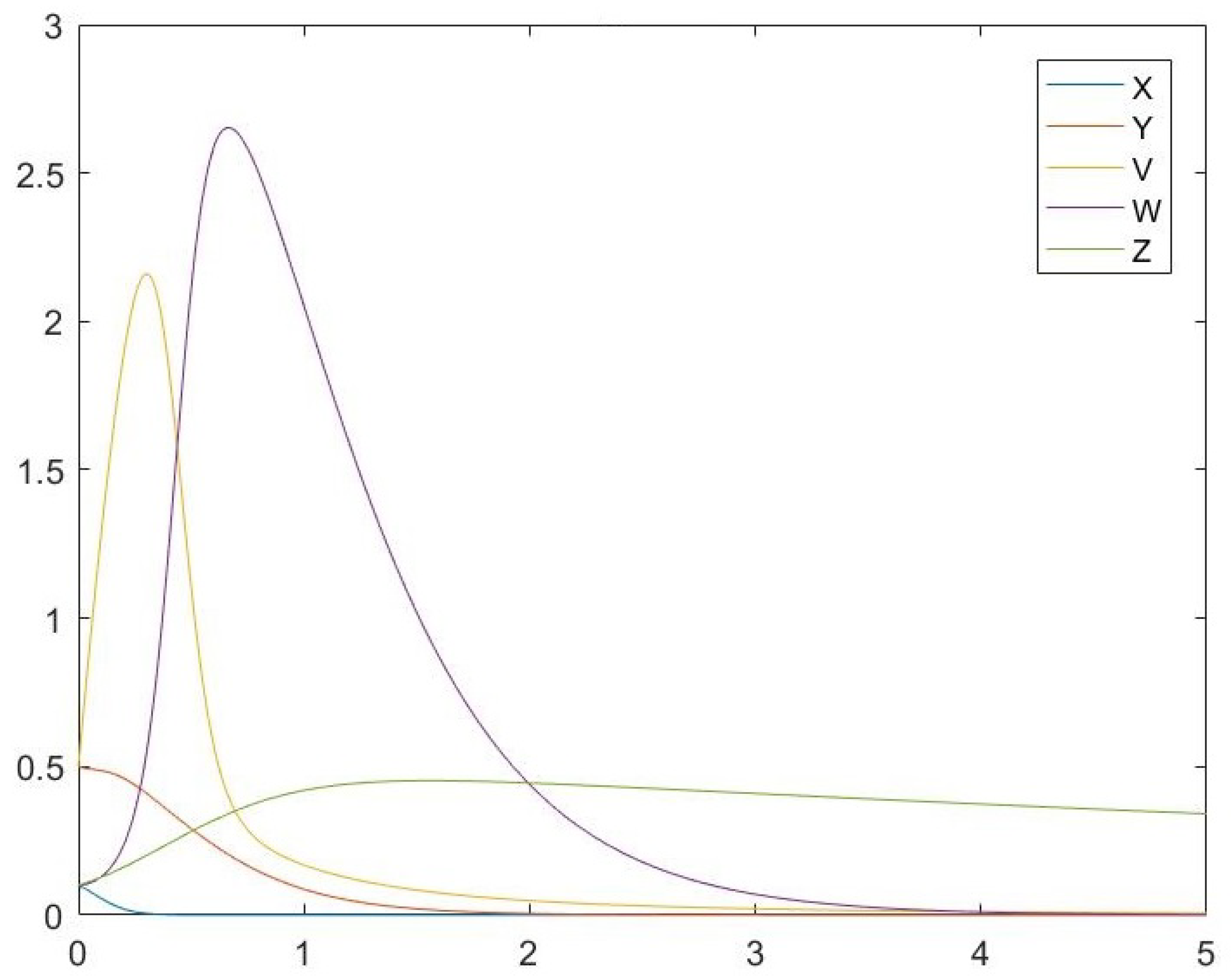
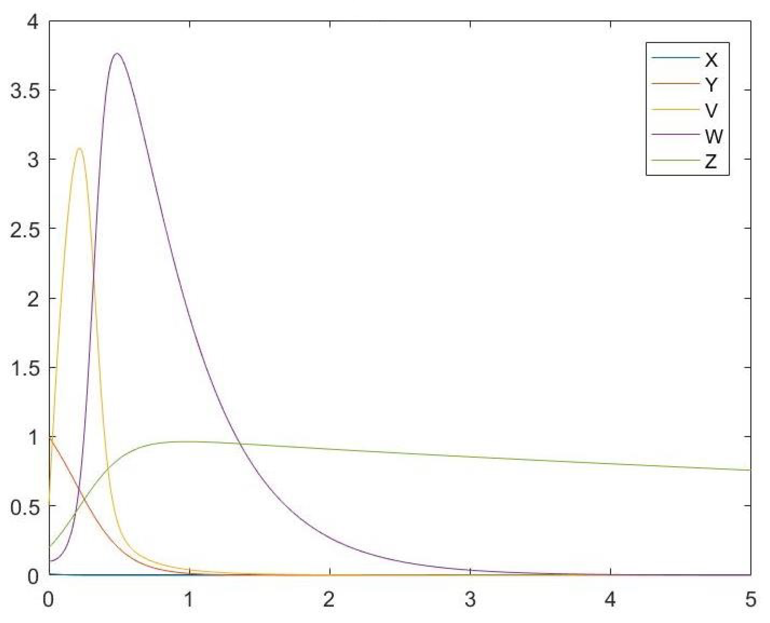
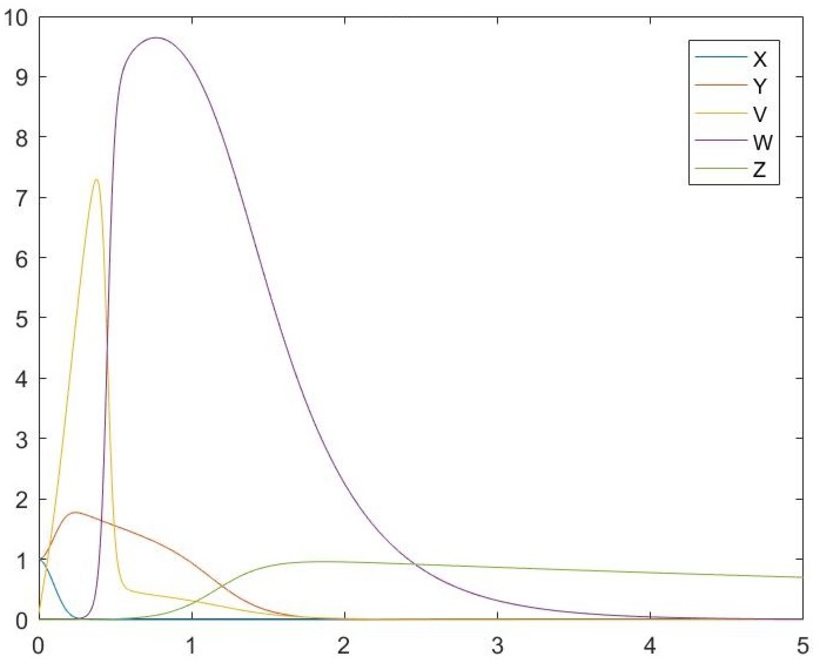
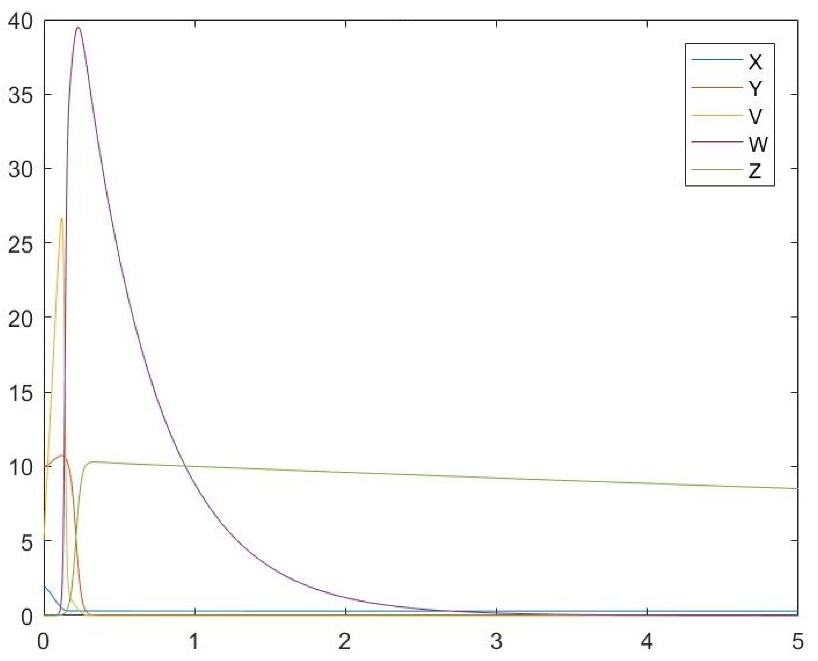
Consider system (3), where

$$U\left(t\right)={\int }_0^{t-\tau \left(t\right)}{e}^{-\alpha (t-s)}Z\left(s\right)ds.$$

(28)

Denote

$$\tilde{U}\left(t\right)={\int }_0^t{e}^{-\alpha (t-s)}Z\left(s\right)ds.$$

(29)

Let us write (28) in the following form:

$$U\left(t\right)=e^{-\alpha \tau \left(t\right)}{\int }_0^{t-\tau \left(t\right)}{e}^{-\alpha \left(\right(t-\tau \left(t\right))-s)}Z\left(s\right)ds=e^{-\alpha \tau \left(t\right)}\tilde{U}(t-\tau \left(t\right)).$$

(30)

Reducing integro-differential system (3), where $U\left(t\right)$ is defined by (28), to an ordinary differential system, I obtain

$$\left\{\begin{array}{c}{X}^{\prime }=r-dX-(1-\eta )\beta VX\hfill \\ Y^{\prime }=(1-\eta )\beta VX-aY-pYZ\hfill \\ V^{\prime }=(1-\epsilon )kY-uV-qVW\hfill \\ W^{\prime }=-hW+gVW\hfill \\ Z^{\prime }=cYZ-bZ+D\tilde{U}+D{e}^{-\alpha \tau \left(t\right)}\tilde{U}(t-\tau \left(t\right))-D\tilde{U}\hfill \\ {\tilde{U}}^{\prime }=Z-\alpha \tilde{U}\hfill \end{array}\right..$$

(31)

Linearizing systems (31) in the neighborhood of the equilibrium free point (6), I obtain the corresponding homogeneous linear systems:

$$\left\{\begin{array}{c}{x}_1^{\prime }\left(t\right)=r-d{x}_1\left(t\right)-\frac{(1-\eta )\beta r}{d}{x}_3\left(t\right)\hfill \\ x_2^{\prime }\left(t\right)=-a{x}_2\left(t\right)+\frac{(1-\eta )\beta r}{d}{x}_3\left(t\right)\hfill \\ x_3^{\prime }\left(t\right)=(1-\epsilon )k{x}_2\left(t\right)-u{x}_3\left(t\right)\hfill \\ x_4^{\prime }\left(t\right)=-h{x}_4\left(t\right)\hfill \\ x_5^{\prime }\left(t\right)=D{x}_6\left(t\right)-b{x}_5\left(t\right)+D{e}^{-\alpha \tau \left(t\right)}{x}_6(t-\tau \left(t\right))-D{x}_6\left(t\right)\hfill \\ x_6^{\prime }\left(t\right)=x_5\left(t\right)-\alpha x_6\left(t\right),\hfill \end{array}\right.$$

(32)

where

$$x_1\left(t\right)=X-\frac{r}{d},x_2\left(t\right)=Y,x_3\left(t\right)=V,x_4\left(t\right)=W,x_5\left(t\right)=Z,x_6\left(t\right)=\tilde{U}$$

Let us denote ${\tau }_{*}=ess{inf}_{t\ge 0}\left|\tau \left(t\right)\right|$ and

$$\left({\mathsf{\Omega }}_2{K}_2\right)\left(t\right)=D{e}^{-\alpha \tau \left(t\right)}{\int }_0^{t-\tau \left(t\right)}\left(c_{28}{e}^{(-c_{13}+c_{14})(t-\tau \left(t\right)-\gamma )}-c_{28}{e}^{(-c_{13}-c_{14})(t-\tau \left(t\right)-\gamma )}\right)k_{2_5}\left(\gamma \right)d\gamma$$

$$D{e}^{-\alpha \tau \left(t\right)}{\int }_0^{t-\tau \left(t\right)}\left(-c_{31}{e}^{(-c_{13}+c_{14})(t-\tau \left(t\right)-\gamma )}+c_{32}{e}^{(-c_{13}-c_{14})(t-\tau \left(t\right)-\gamma )}\right)k_{2_6}\left(\gamma \right)d\gamma$$

$$-D{\int }_0^t\left(c_{28}{e}^{(-c_{13}+c_{14})(t-\gamma )}-c_{28}{e}^{(-c_{13}-c_{14})(t-\gamma )}\right)k_{2_5}\left(\gamma \right)d\gamma$$

$$-D{\int }_0^t\left(-c_{31}{e}^{(-c_{13}+c_{14})(t-\gamma )}+c_{32}{e}^{(-c_{13}-c_{14})(t-\gamma )}\right)k_{2_6}\left(\gamma \right)d\gamma .$$

$$Q_2=D{e}^{\alpha {\tau }_{*}}\left(\left|\frac{c_{28}}{c_{14}-c_{13}}\right|+\left|\frac{c_{28}}{c_{13}+c_{14}}\right|+\left|\frac{c_{31}}{c_{14}-c_{13}}\right|+\left|\frac{c_{32}}{c_{13}+c_{14}}\right|\right)$$

$$+D\left(2\left|c_{28}\right|+\left|c_{31}\right|+\left|c_{32}\right|\right)$$

Theorem 5.

If all of the coefficients of system (5) are positive; η and ε are parameters defined between 0 to 1; and inequalities (15), (16), and $Q_2<1$ are fulfilled, then system (31) is exponentially stable.

Proof. 

I can write system (10) in the following form:

$$X^{\prime }\left(t\right)=AX\left(t\right),$$

(33)

where

$$X\left(t\right)=col\{x_1\left(t\right),x_2\left(t\right),x_3\left(t\right),x_4\left(t\right),x_5\left(t\right),x_6\left(t\right)\},$$

and A defined by (12).

It is known that the general solution of the system

$$X^{\prime }\left(t\right)-AX\left(t\right)=K_2\left(t\right)$$

(34)

can be represented in the following form:

$$X\left(t\right)={\int }_0^{t}C(t,\gamma )K_2\left(\gamma \right)d\gamma +C(t,0)X\left(0\right)$$

(35)

where $C(t,s)$ is a Cauchy matrix (23) of system (10). I can rewrite system (32) in the following form:

$$\left\{\begin{array}{c}{x}_1^{\prime }\left(t\right)+d{x}_1\left(t\right)+\frac{(1-\eta )\beta r}{d}{x}_3\left(t\right)=r\hfill \\ x_2^{\prime }\left(t\right)+a{x}_2\left(t\right)-\frac{(1-\eta )\beta r}{d}{x}_3\left(t\right)=0\hfill \\ x_3^{\prime }\left(t\right)-(1-\epsilon )k{x}_2\left(t\right)+u{x}_3\left(t\right)=0\hfill \\ x_4^{\prime }\left(t\right)+h{x}_4\left(t\right)=0\hfill \\ x_5^{\prime }\left(t\right)-D{x}_6\left(t\right)+b{x}_5\left(t\right)=D{e}^{-\alpha \tau \left(t\right)}{x}_6(t-\tau \left(t\right))-D{x}_6\left(t\right)\hfill \\ x_6^{\prime }\left(t\right)-x_5\left(t\right)+\alpha x_6\left(t\right)=0\hfill \end{array}\right.$$

(36)

Without loss of generality, I assume that $X\left(0\right)=0$.

Substituting $X\left(t\right)={\int }_0^{t}C(t,\gamma )K_2\left(\gamma \right)d\gamma$ into system (36), I have

$$x_6(t-\tau \left(t\right))=\sum _{i=1}^6{\int }_0^{t-\tau \left(t\right)}{c}_{6i}((t-\tau \left(t\right)),\gamma )k_{2_i}\left(\gamma \right)d\gamma$$

and the following system for $K_2\left(t\right)$:

$$K_2\left(t\right)=\left({\mathsf{\Omega }}_2{K}_2\right)\left(t\right)+F_2\left(t\right),$$

where

$$K_2\left(t\right)=\left(\begin{array}{c}{k}_{2_1}\left(t\right)\\ k_{2_2}\left(t\right)\\ k_{2_3}\left(t\right)\\ k_{2_4}\left(t\right)\\ k_{2_5}\left(t\right)\\ k_{2_6}\left(t\right)\end{array}\right),F_2\left(t\right)=\left(\begin{array}{c}r\\ 0\\ 0\\ 0\\ 0\\ 0\end{array}\right),$$

and the operator ${\mathsf{\Omega }}_2:L_{\infty }⟶L_{\infty }$ is defined by

$$\left({\mathsf{\Omega }}_2{K}_2\right)\left(t\right)=\left(\begin{array}{c}0\\ 0\\ 0\\ 0\\ {\omega }_2{K}_2\left(t\right)\\ 0,\end{array}\right)$$

where

$$\left({\mathsf{\Omega }}_2{K}_2\right)\left(t\right)=D{e}^{-\alpha \tau \left(t\right)}{\int }_0^{t-\tau \left(t\right)}\left(c_{28}{e}^{(-c_{13}+c_{14})(t-\tau \left(t\right)-\gamma )}-c_{28}{e}^{(-c_{13}-c_{14})(t-\tau \left(t\right)-\gamma )}\right)k_{2_5}\left(\gamma \right)d\gamma$$

$$D{e}^{-\alpha \tau \left(t\right)}{\int }_0^{t-\tau \left(t\right)}\left(-c_{31}{e}^{(-c_{13}+c_{14})(t-\tau \left(t\right)-\gamma )}+c_{32}{e}^{(-c_{13}-c_{14})(t-\tau \left(t\right)-\gamma )}\right)k_{2_6}\left(\gamma \right)d\gamma$$

$$-D{\int }_0^t\left(c_{28}{e}^{(-c_{13}+c_{14})(t-\gamma )}-c_{28}{e}^{(-c_{13}-c_{14})(t-\gamma )}\right)k_{2_5}\left(\gamma \right)d\gamma$$

$$-D{\int }_0^t\left(-c_{31}{e}^{(-c_{13}+c_{14})(t-\gamma )}+c_{32}{e}^{(-c_{13}-c_{14})(t-\gamma )}\right)k_{2_6}\left(\gamma \right)d\gamma .$$

according to (23). Estimating the norm of the operator ${\mathsf{\Omega }}_2$, I obtain the assertion of this theorem. □

6. Simulations

In order to validate the proposed model (3), I chose a validation set defined by the initial conditions and dose of the drugs.

Set 1: initial conditions $X\left(0\right)=0.5,Y\left(0\right)=0.1,V\left(0\right)=0.1,W\left(0\right)=0.1,Z\left(0\right)=0.1,$ and $U\left(0\right)=0.1$ and dose of the drugs $ϵ=0.5,\eta =0.5,\alpha =2,$ and $D=0.1$.

Set 2: initial conditions $X\left(0\right)=0.1,Y\left(0\right)=0.5,V\left(0\right)=0.5,W\left(0\right)=0.1,Z\left(0\right)=0.1,$ and $U\left(0\right)=0$ and dose of the drugs $ϵ=0.1,\eta =0.1,\alpha =10,$ and $D=0.2$.

Set 3: initial conditions $X\left(0\right)=0.01,Y\left(0\right)=0.9,V\left(0\right)=0.2,W\left(0\right)=0.01,Z\left(0\right)=0.1,$ and $U\left(0\right)=0.2$ and dose of the drugs $ϵ=0.01,\eta =0.02,\alpha =5,$ and $D=0.01$.

Set 4: initial conditions $X\left(0\right)=0.01,Y\left(0\right)=1,V\left(0\right)=0.5,W\left(0\right)=0.1,Z\left(0\right)=0.2,U\left(0\right)=0.5$ and doze of the drugs $ϵ=0.001,\eta =0.1,\alpha =1,D=0.05$.

Set 5: initial conditions $X\left(0\right)=1,Y\left(0\right)=1,V\left(0\right)=0.1,W\left(0\right)=0.001,Z\left(0\right)=0.0002,$ and $U\left(0\right)=0.0001$ and dose of the drugs $ϵ=0.25,\eta =0.1,\alpha =2,$ and $D=0.01$.

Set 6: initial conditions $X\left(0\right)=2,Y\left(0\right)=10,V\left(0\right)=5,W\left(0\right)=0.0001,Z\left(0\right)=0.0001,$ and $U\left(0\right)=0.0001$ and dose of the drugs $ϵ=0.01,\eta =0.9,\alpha =7,$ and $D=0.5$.

Set 7: initial conditions $X\left(0\right)=0.1,Y\left(0\right)=10,V\left(0\right)=5,W\left(0\right)=0.1,Z\left(0\right)=0.01,$ and $U\left(0\right)=1$ and dose of the drugs $ϵ=0.9,\eta =0.1,\alpha =0.1,$ and $D=0.001$.

Set 8: initial conditions $X\left(0\right)=1,Y\left(0\right)=2,V\left(0\right)=0.1,W\left(0\right)=0.1,Z\left(0\right)=0.2,$ and $U\left(0\right)=0.1$ and dose of the drugs $ϵ=0.2,\eta =0.8,\alpha =0.5,$ and $D=0.005$.

Remark 1.

From [20], I used the following values of the parameters in system (1):

$$d=0.00333,g=q=5,b=0.112,\beta =7,h=2,a=0.56,u=0.67,p=c=5.14,$$

$$k=20,r=6.17*{10}^{-4}.$$

The results of the simulations are presented in Figure 1, Figure 2, Figure 3, Figure 4, Figure 5, Figure 6, Figure 7 and Figure 8 accordingly.

7. Conclusions

In this paper, I presented a mathematical model for HBV infection, considering a possible co-treatment with the standard of care and IL-2 and using distributed control with unbounded memory.

In Section 2, I obtained the relation between the convergence rate of system (1) and modified system (3). I obtained a faster stability convergence for system (3) in the stability state; thus, patients can achieve faster improvements in their health conditions.

In Section 3 and Section 4, I obtained the exponential stability of system (3) using the proposed distributed control with unbounded memory. A delay in the upper or lower limits of the integral can show the start and end periods of patient treatment. I showed estimates of this delay such that a patient achieves stabilization in their health condition and improvements.

In Section 5, I presented the simulations, where the chosen parameters of system (3) satisfy the conditions of Theorem 2. The results of the simulations on the validation set show that the chosen treatment stabilizes a patient’s health condition.

References

1. Tang, L.S.Y.; Covert, E.; Wilson, E.; Kottilil, S. Chronic Hepatitis B Infection: A Review. JAMA 2018, 319, 1802–1813. [Google Scholar] [CrossRef] [PubMed]
2. Long, C.; Qi, H.; Huang, S.H. Mathematical modeling of cytotoxic lymphocyte-mediated immune response to hepatitis B virus infection. J. Biomed. Biotechnol. 2008, 2008, 743690. [Google Scholar] [CrossRef] [PubMed] [Green Version]
3. Poh, Z.; Goh, B.B.; Chang, P.E.; Tan, C.K. Rates of cirrhosis and hepatocellular carcinoma in chronic hepatitis B and the role of surveillance: A 10-year follow-up of 673 patients. Eur. J. Gastroenterol. Hepatol. 2015, 27, 638–643. [Google Scholar] [CrossRef] [PubMed] [Green Version]
4. Parkin, D.M. The global health burden of infection-associated cancers in the year 2002. Int. J. Cancer 2006, 118, 3030–3044. [Google Scholar] [CrossRef] [PubMed] [Green Version]
5. European Association for the Study of the Liver. EASL 2017 Clinical Practice Guidelines on the management of hepatitis B virus infection. J. Hepatol. 2017, 67, 370–398. [Google Scholar] [CrossRef] [Green Version]
6. Berezansky, L.; Bunimovich-Mendrazitsky, S.; Schklar, B. Stability and controllability issues in mathematical modeling of the intensive treatment of leukemia. J. Optim. Theory Appl. 2015, 167, 326–341. [Google Scholar] [CrossRef]
7. Berezansky, L.; Bunimovich-Mendrazitsky, S.; Domoshnitsky, A. A mathematical model with time-varying delays in the combined treatment of chronic myeloid leukemia. Adv. Differ. Equ. 2012, 217, 1–13. [Google Scholar] [CrossRef] [Green Version]
8. Bershadsky, M.; Chirkov, M.; Domoshnitsky, A.; Rusakov, S.; Volinsky, I. Distributed Control and the Lyapunov Characteristic Exponents in the Model of Infectious Diseases. Complexity 2019, 2019, 5234854. [Google Scholar] [CrossRef]
9. Bunimovich-Mendrazitsky, S.; Kronik, N.; Vainstein, V. Optimization of interferon-alpha and imatinib combination therapy for chronic myeloid leukemia: A modeling approach. Adv. Theory Simul. 2019, 2, 1800081. [Google Scholar] [CrossRef]
10. Bunimovich-Mendrazitsky, S.; Goltser, Y. Use of quasi-normal form to examine stability of tumor-free equilibrium in a mathematical model of BCG treatment of bladder cancer. Math. Biosci. Eng. 2011, 8, 529–547. [Google Scholar] [CrossRef] [PubMed]
11. Domoshnitsky, A.; Volinsky, I.; Bershadsky, M. Around the Model of Infection Disease: The Cauchy Matrix and Its Properties. Symmetry 2019, 11, 1016. [Google Scholar] [CrossRef] [Green Version]
12. Domoshnitsky, A.; Volinsky, I.; Pinhasov, O. Some developments in the model of testosterone regulation. AIP Conf. Proc. 2019, 2159, 030010. [Google Scholar] [CrossRef]
13. Domoshnitsky, A.; Volinsky, I.; Pinhasov, O.; Bershadsky, M. Questions of Stability of Functional Differential Systems around the Model of Testosterone Regulation. Bound. Value Probl. 2019, 1, 1–13. [Google Scholar] [CrossRef]
14. Colombatto, P.; Civitano, L.; Bizzarri, R.; Oliveri, F.; Choudhury, S.; Gieschke, R.; Bonino, F.; Brunetto, M.R.; Peginterferon Alfa-2a HBeAg-Negative Chronic Hepatitis B Study Group. A multiphase model of the dynamics of HBV infection in HBeAg-negative patients during pegylated interferon-α, lamivudine and combination therapy. Antivir. Ther. 2006, 11, 197–212. [Google Scholar] [PubMed]
15. Nowak, M.A.; Bonhoeffer, S.; Hill, A.M.; Boehme, R.; Thomas, H.C.; McDade, H. Viral dynamics in hepatitis B virus infection. Proc. Natl. Acad. Sci. USA 1996, 93, 4398–4402. [Google Scholar] [CrossRef] [PubMed] [Green Version]
16. Perelson, A.S.; Ribeiro, R.M. Hepatitis B virus kinetics and mathematical modeling. Semin. Liver Dis. 2004, 24, 11–16. [Google Scholar] [CrossRef] [PubMed]
17. Wain-Hobson, S. Virus Dynamics: Mathematical Principles of Immunology and Virology. Nat. Med. 2001, 7, 525–526. [Google Scholar] [CrossRef]
18. Yousdi, N.; Hattaf, K.; Rachik, M. Analysis of a HCV model with CTL and antibody responses. Appl. Math. Sci. 2009, 3, 2835–2845. [Google Scholar]
19. Volinsky, I.; Lombardo, S.D.; Cheredman, P. Stability Analysis and Cauchy Matrix of a Mathematical Model of Hepatitis B Virus with Control on Immune System near Neighborhood of Equilibrium Free Point. Symmetry 2021, 13, 166. [Google Scholar] [CrossRef]
20. Chenar, F.F.; Kyrychko, Y.N.; Blyuss, K.B. Mathematical model of immune response to hepatitis B. J. Theor. Biol. 2018, 447, 98–110. [Google Scholar] [CrossRef] [PubMed] [Green Version]
Figure 1. Set 1.
Symmetry 13 01437 g001
Figure 2. Set 2.
Symmetry 13 01437 g002
Figure 3. Set 3.
Symmetry 13 01437 g003
Figure 4. Set 4.
Symmetry 13 01437 g004
Figure 5. Set 5.
Symmetry 13 01437 g005
Figure 6. Set 6.
Symmetry 13 01437 g006
Figure 7. Set 7.
Symmetry 13 01437 g007
Figure 8. Set 8.
Symmetry 13 01437 g008
Publisher’s Note: MDPI stays neutral with regard to jurisdictional claims in published maps and institutional affiliations.