Article

Lensless Reflection Imaging of Obliquely Illuminated Objects I: Choosing a Domain for Phase Retrieval and Ptychography

by
Igor A. Artyukov
,
Nikolay L. Popov
* and
Alexander V. Vinogradov
P.N. Lebedev Physical Institute, Leninsky Prospekt 53, 119991 Moscow, Russia
*
Author to whom correspondence should be addressed.
Symmetry 2021, 13(8), 1439; https://doi.org/10.3390/sym13081439
Submission received: 16 June 2021 / Revised: 27 July 2021 / Accepted: 29 July 2021 / Published: 5 August 2021

Abstract

:
Ptychography is a lensless imaging technology that is validated from hard X-rays to terahertz spectral range. It is most attractive for extreme ultraviolet (EUV) and X-rays as optical elements are expensive and often not available. Typically, the set up involves coherently illuminated object that directs the scattered radiation normally to detector which is parallel to the object plane. Computer processing of diffraction patterns obtained when scanning the object gives the image, more precisely, the distribution of intensity and phase on its surface. However, this scheme is inefficient for EUV and X-rays due to poor reflectivity and low penetration in all materials. Reflection mode ptychography solves the problem if illumination angles do not exceed the critical angle of object material. Changing the geometry of experiment changes physical and mathematical model of image formation. Including: diffraction integral describing beam propagation from object to detector, inverse problem, optimization of object illumination angle, position and orientation of detector, choosing size and grid of coordinate and frequency computer domains. This paper considers the wavefield scattered to detector by obliquely illuminated object and determines a domain for processing of obtained scans. Solution of inverse problem with phase retrieval and resulting numerical images will be presented in the next paper.

1. Introduction

The retrieval of the field phase on the object under study, is a basis of modern lensless imaging. Ideally, the task is formulated as follows: to restore the phase of the coherent wave field from the measurements of its modulus on two parallel planes determined by the object and the detector. For this purpose, the iterative algorithm is used with calculation of the propagation of coherent radiation from the object plane to the plane of the detector. The result is the distribution of the complex field on both planes. This problem was solved for the first time, in [1] using one of the best computers at that time with ~1 megabyte memory and ~1 megaflop performance, which made it possible to analyze a large number of 32 × 32 images. The development of the ideas of this work led to the emergence of lensless imaging and ptychography as they are currently used in the visible, EUV and X-ray ranges [2,3,4,5,6,7,8,9]. Since 1970s the original algorithm [1] has been improved to be more efficient, following the progress in computer technology. New algorithms were developed to avoid the need for measurement of the intensity distribution on the object plane and to replace it by a priori information. As a result, lensless imaging methods had become applicable in a number of physics research and commercial projects [10,11,12,13]. One of the main advantages of lensless optical systems is the fundamental possibility to get rid of a problem associated with aberrations of imaging optical elements in approaching the diffraction resolution limit in microscopy, atmospheric and astronomical optics (Obviously, in order to fully realize the indicated advantage of lensless systems, it is necessary to go beyond the paraxial methods of modeling the propagation of light beams from an object to a detector).
Over the past 10–15 years, ptychography has become one of the most popular and rapidly developing lensless imaging technologies. Its scheme is shown in Figure 1. In the simplest case, ptychography consists of a registration of a sequence of interference patterns collected upon illuminating the object at partially overlapping positions produced by an object moving across a coherent beam spot, with the radiation source and detector position being fixed. Thus, the image is determined to be a distribution of the complex field amplitude (i.e., modulus and phase) on the surface of an object. It can be obtained as a result of computer processing of a set of the patterns. Using a sequence of overlapping scans instead of a single measured pattern (as in common phase retrieval method) allows one to omit a priori suggestions concerning the object optical properties.
The principles of ptychography and the very term were proposed in the works of Hoppe et al. [14,15]. However, for a long time this approach remained unnoticed due to the lack of an effective algorithm for its implementation. Such algorithm was proposed only in 2004 [16,17]. This algorithm is now known as the Ptychography Iterative Engine (PIE). However, the algorithm has a drawback—it assumes that the illuminating field is known. After 4 years, in 2008, this problem was fixed in another iterative algorithm based on the difference map approach [18,19]. In 2009 an improved algorithm PIE—Extended Ptychography Iterative Engine (ePIE)—was proposed [20].
Today ptychography is a widely used microscopy method that provides a complete (amplitude and phase) description of flat objects. Its field of application extends from terahertz [21] to hard X-rays [9]. Since there are no optical elements used, the spatial resolution is limited only by the wavelength and the detector parameters. These advantages make ptychography an attractive technique and stimulate new applications and, imaging technology (see books [22,23], review [24], and also [25]). Let us now turn to the content of this work.
The basic idea underlying ptychography and other phase reconstruction methods is the unambiguity of solving the inverse diffraction problem for the scalar wave equation; that is, unambiguous reconstruction of the complex field near the object from the known complex field near the detector. In the case of a normal location of the object, when the planes of the object and the detector are parallel and at the same time perpendicular to the beam, unambiguity is usually beyond doubt and corresponding wave field distributions are linked by the Fresnel transformations. However, in the case of an oblique position of the object to the ray (see Figure 1), the task gets more complicated. As shown in [26], the inverse problem in paraxial approximation is reduced to solving the singular integral equation.
The second idea underlying the phase reconstruction methods is the numerical calculation of the complex field near the detector from the known complex field near the object and vice versa. All currently known effective methods of such calculations are based on the fast Fourier transform [27,28,29]. For such calculations, complex fields are specified on finite lattices (digital domains). If one of the two domains is specified on either the object or the detector, then the other domain, obviously, must be dependent on it. Unfortunately, in the literature, these formulas, as well as the principles of domain selection, were not presented for an oblique object.
In the present work, within the framework of the Helmholtz equation, we propose a criterion for the uniqueness of the inverse problem solution. As well we present the formulas for calculating diffraction by a tilted object for the case of large apertures and large distances in high resolution ptychography. These formulas include the calculation of the detector domain from the object domain parameters as a development of the formulas obtained for a vertical object in our previous work [30].

2. Materials and Methods

2.1. Phase and Modulus Retrieval of Normally Located Object

Most of the modern methods of phase retrieval are, a further development of the algorithms created 30–40 years ago (see the literature cited in [20,24] and [31,32,33]). These algorithms are presented in many articles and monographs and continue to be improved. They assume that the registration of the field intensity distribution on the detector explicitly determines the modulus of the Fourier image of the field on the object in a certain range of the spatial frequencies.
The algorithms contain 4 basic operations on the complex object function f : (a) the Fourier transform F , (b) replacing its modulus with the experimentally obtained value A , (c) the inverse Fourier transform F 1 and (d) the P transform of the function f , that is a priori information about the object. The result of these transformations is a new function
f = P [ F 1 [ A F [ f ] | F [ f ] | ] ]
defined in the same domain as f . If f and f coincide with the specified precision, then the goal is achieved. A priori information ( P ) can be the measurement of the field modulus directly behind the object or in any other plane, the shape of the object, that is, equality to zero of the field on the object plane outside a definite area, non-negative values of the field, etc.
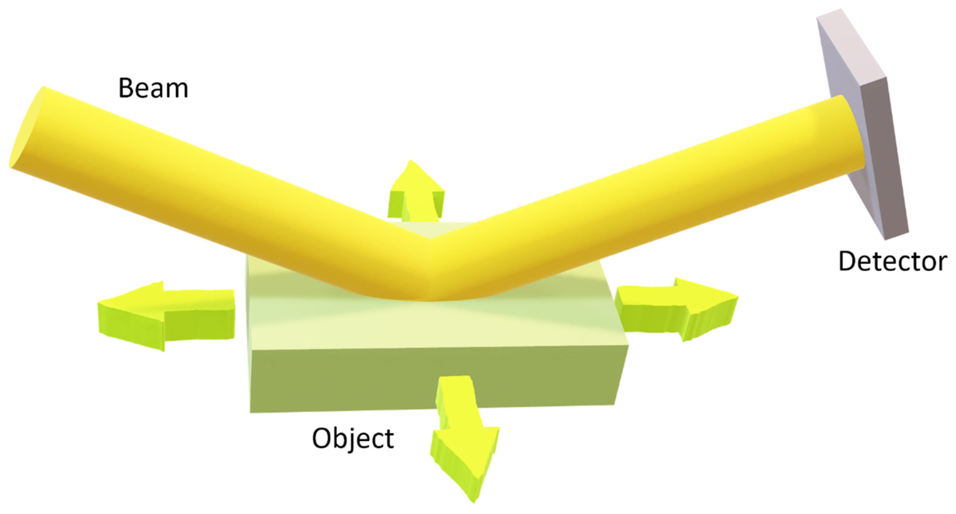
The diagram of a typical diffraction-resolved lensless imaging microscope contains a coherent radiation source illuminating a transparent object located in the S plane (see Figure 2). Unlike conventional microscopes, there are no optical elements between the object and the detector. The laser illuminating the object on the left and the computer processing the data from the detector are not shown in the diagram.
Let us show the role of the Fourier transform using the example of an angular spectrum that describes the propagation of coherent radiation from an object S to a detector S (see Figure 2) and is an exact, and consequently, nonparaxial solution of the wave equation. It defines the wave field in a half-space through spatial harmonics in the object plane:
ψ ( r ) = φ 0 ( p ) d 2 p e x p { i p ρ + i k 2 p 2 z } , r = ( x , y , z ) = ( ρ , z ) ,
where k = 2 π λ is the wave number, φ 0 ( p ) is the Fourier transform of the field distribution ψ ( ρ ,   z = 0 ) in the object plane. Papers [29,34,35,36] are devoted to the analysis of this expression and its connection with other forms of the diffraction integral. Here we will consider only issues related to modeling the propagation of non-paraxial beams in the problems of image phase reconstruction and ptychography.
Assume that the detector recording the intensity is in the far zone of the object, i.e., in the Fourier plane, where:
z a 2 λ ,   ρ = z tan θ a ,
a is the size of the object, and the aperture angle θ a is assumed to be fixed. Considering (2) under condition (3) and using the stationary phase method [37], it is easy to make sure that the field at the detector takes the form:
ψ ( ρ , z ) = 2 π k i z z 2 z 2 + ρ 2 e x p { i k z 2 + ρ 2 } φ 0 ( p = k ρ z 2 + ρ 2 ) .
Expression (4), obtained from the exact solution (2) of the Helmholtz wave equation, shows that in the far zone the spatial distribution of the field ψ ( ρ , z ) is expressed through the Fourier transform φ 0 ( p ) of the field on the object plane ψ ( ρ , 0 ) . Moreover, when the coordinate ρ on the detector changes from 0 to , the corresponding spatial harmonic p changes from 0 to k . In other words, there are no harmonics p > k in the far field. In the general case, this expresses the fact that the limiting spatial resolution in the far zone is determined by the wavelength λ = 2 π k , regardless of the type of optical system.
In practice, in phase retrieval algorithms (see review [31]), to avoid the computational complexity of exact Expression (4), a simpler one is used—the Fresnel integral, which follows from exact Expression (2) at small aperture angles θ a :
ψ ( ρ , z ) = k e i k z 2 π i z ψ ( ρ , 0 ) d 2 ρ e x p { i k ( ρ ρ ) 2 2 z } ,
that in the far field (3) has the form:
ψ ( ρ , z ) = 2 π k i z e x p { i k z ( 1 + ρ 2 2 z 2 ) } φ 0 ( p = k ρ z ) .
Let us compare the obtained expression (6) with the exact value of the field in the far zone (4). Comparison of the arguments of the Fourier transform of the initial distribution φ 0 ( p ) shows that the use of the Fresnel integral in the far zone (6) for calculating the field at the detector is possible only for ρ z , i.e., θ a 45 ° and aperture N A = sin θ a 0.71 . Otherwise, we would be talking about the harmonics of the initial distribution p > k which, according to (4), are not contained in the far zone at all. Adding to this the requirement that the phase factors in (4) and (6) coincide, we obtain the condition for the applicability of the Fresnel integral in the far field (3), (see [38]):
tan θ a 1 ,     a 2 λ z 4 π λ tan 4 θ a
A more detailed theoretical discussion of the issue is available in review [39].
Thus, the angular spectrum approximation (4), as well as the paraxial approximation (6), in the far zone lead to the aforementioned connection between the field intensity distribution at the detector and the Fourier transform module of the field in the object plane. Namely, the intensity on the detector is algebraically expressed through the Fourier transform of the field amplitude on the object.

2.2. Angular Spectrum and Oblique Object

Consider the propagation of reflected directional monochromatic radiation from a tilted opaque object as shown in Figure 3. The surface of the object is located on plane S in the half-plane s > 0 , the detector is on the S plane at z = 0 . The plane S is inclined to the plane x = 0 at an angle of θ , and to the plane of the detector at an angle of π / 2 θ . Without loss of generality, one can suggest 0 < θ < π / 2 . This can be achieved by choosing the appropriate coordinate system. Then, we will assume that the radiation is described by the scalar function ψ ( x , y , z ) , which is a solution of the Helmholtz equation:
2 ψ x 2 + 2 ψ y 2 + 2 ψ z 2 + k 2 ψ = 0 , k = 2 π λ .
We also assume that the radiation propagates in the direction of increasing z from left to right being a superposition
ψ ( x , y , z ) = d p x d p y Ψ ( p x , p y ) ψ p ( x , y , z )
of the plane waves (“angular spectrum method”) with transverse momentum p = ( p x , p y ) T
ψ p ( x , y , z ) = e i p x x + i p y y + i k 2 p x 2 p y 2 z .
One can see that the function Ψ ( p x , p y ) is the Fourier transform of the function ψ ( x , y , 0 ) . The fact that the plane wave (10) propagates in the direction of increasing z is expressed by the plus sign in front of the square root in the exponent. Let us denote unit vectors along the x , y , z , s axes as e x , e y , e z , e s , respectively. Then the 3D wave vector is p = p x e x + p y e y + k 2 p x 2 p y 2 e z . The plane of the object divides the space into a conditionally upper half-space, where x z   tan θ and the lower one, where x < z   tan θ . We denote the quantities referring to the upper half-space by the “ + ” sign at the bottom, and the lower half-space by the “ ” sign at the bottom. Occurrence of the wave ψ p in the positive half-space is formulated as the condition:
R e ( ( p ( p · e s ) e s ( p · e y ) e y ) e z ) 0 ,
where R e is the real part, since p is complex in general case. Considering that e s = cos θ e z + sin θ e x we express (11) through the angles:
R e ( sin θ ( p ˜ x cos θ + 1 p ˜ x 2 p ˜ y 2 sin θ ) ) 0 .
where, for convenience, we introduced the dimensionless parameter p ˜ = p / k = ( p ˜ x , p ˜ y , p ˜ z ) T . Then, the symbol “~” at the top will denote quantities divided by k . We introduce new notation: complex angles ϑ and φ that satisfy the conditions:
sin ϑ = p ˜ x cos θ + 1 p ˜ x 2 p ˜ y 2 sin θ ,
cos φ = p ˜ x sin θ 1 p ˜ x 2 p ˜ y 2 cos θ .
From Equations (13) and (14) we can express p ˜ x through the angles ϑ and φ :
p ˜ x = sin ϑ cos θ + cos φ sin θ ,
Using Equation (13), the condition (12) can be written as:
R e ( sin θ sin ϑ ) 0 .
For | p | k the vector p ˜ is real. Then, the angle ϑ is equal to the angle of inclination p ˜ to the plane of the object, and the angle φ is equal to the angle of inclination p ˜ to the s axis (see Figure 3). For all angles 0 < θ < π / 2 , the condition (16) is equivalent to the condition ϑ     0 , that means a wave, either leaving the object in the upper half-space for ϑ > 0 , or surface wave moving along the object from top to bottom at ϑ = 0 . The angular spectrum ψ can be represented as an integral of plane waves (9) and as a product of the slow and fast parts:
ψ ( x , y , z ) = u ( x , y , z ) e i k z .
In what follows, we will be interested in the evolution of the slow part u ( x , y , z ) more suitable for numerical calculations. The slow part of the plane wave looks like this:
u p ˜ ( x , y , z ) = e i k ( p ˜ x x + p ˜ y y + ( 1 p ˜ x 2 p ˜ y 2 1 ) z ) .
Suppose that the field of the exit wave of the object is known — it is the function u ( s , y ) = u ( x = s sin θ , y , z = s cos θ ) defined on the plane S . To obtain the field on the detector u ( x , y , 0 ) we will find an arbitrary harmonic q ˜ = ( q ˜ s , q ˜ y ) T :
u q ˜ ( s , y ) = e i k ( q ˜ s s + q ˜ y y ) .
Substituting x = s sin θ , z = s cos θ into (18) we get:
u q ˜ ( s , y ) = e i k ( ( p ˜ x sin θ ( 1 p ˜ x 2 p ˜ y 2 1 ) cos θ ) s + p ˜ y y ) .
From Equations (19) and (20) we obtain the equations connecting p ˜ and q ˜ :
q ˜ = ( p ˜ x sin θ ( 1 p ˜ x 2 p ˜ y 2 1 ) cos θ , p ˜ y ) T ,
p ˜ + , = ( ± cos θ 1 ( q ˜ s cos θ ) 2 q ˜ y 2 + sin θ ( q ˜ s cos θ ) , q ˜ y ) T .
Using Equation (14), we rewrite Equations (21) and (22) in the form:
q ˜ = ( cos φ + cos θ , p ˜ y ) T ,
p ˜ + , = ( ± cos θ 1 ( q ˜ s cos θ ) 2 q ˜ y 2 + sin θ cos φ , q ˜ y ) T ,
It follows from Equations (24) and (15) that:
sin ϑ + , = ± 1 ( q ˜ s cos θ ) 2 q ˜ y 2 .
Thus, for each harmonic q ˜ there are two solutions. One of them, according to Equations (25) and (16), corresponds to a plane wave in the upper half-space, where sin ϑ + 0 , and the other to a plane wave in the lower half-space, where sin ϑ 0 . Since we consider the object to be opaque, we can assume that the wave with ϑ + corresponds to the reflected wave, and the wave in the lower half-space with ϑ does not exist. Therefore, choose p ˜ + :
p ˜ = ( cos θ 1 ( q ˜ s cos θ ) 2 q ˜ y 2 + sin θ ( q ˜ s cos θ ) , q ˜ y ) T .
It is easy to see that the imaginary part p ˜ and 1 | p ˜ | 2 is non-negative for all θ [ 0 , π / 2 ] . From Equation (21), I m ( q ˜ s ) = 0 and Equation (26) we obtain:
I m ( 1 | p ˜ | 2 ) = I m ( p ˜ x ) tan θ ,
I m ( p ˜ x ) = { 0 , ( q ˜ s cos θ ) 2 + q ˜ y 2   1 cos θ ( q ˜ s cos θ ) 2 q ˜ y 2 1 , ( q ˜ s cos θ ) 2 + q ˜ y 2 > 1       .
According to Equation (18), it follows that waves with complex p ˜ would decay exponentially with increasing x and z , so that the information about the corresponding frequencies q does not reach the detector. Therefore, an unambiguous reconstruction of the u ( s , y ) field from the u ( x , y , 0 ) field needs I m ( p ˜ ) = 0 :
( q ˜ s cos θ ) 2 + q ˜ y 2   1 .
Let us suppose that δ s and δ y are the size of the smallest detail of the object u ( s , y ) along the directions s and y , correspondingly (see Figure 4). Then the spectrum is restricted by the Nyquist theorem:
π δ s q s π δ s π δ y q y π δ y ,
λ 2 δ s q ˜ s λ 2 δ s λ 2 δ y q ˜ y λ 2 δ y .
Condition (29) is satisfied for all q ˜ from Equation (31) when:
1 ( λ 2 δ y ) 2 + λ 2 δ s cos θ 1 ( λ 2 δ y ) 2 λ 2 δ s .
In what follows, we will assume that the object is non-crystalline, and its surface changes on a scale larger than the wavelength, and λ / δ s < 1 , λ / δ y < 1 . Then, with taking into account θ [ 0 , π / 2 ] the expression (32) takes the form:
cos θ 1 ( λ 2 δ y ) 2 λ 2 δ s ,
This inequality can be rewritten by introducing the dimensionless parameter Φ :
Φ = 1 + λ 2 δ s 1 ( λ 2 δ y ) 2 1 cos θ 1 .
Expanding by small parameters λ / ( 2 δ s ) and λ / ( 2 δ y ) and taking into account only the first terms, we can get:
Φ λ 2 δ s ( 1 cos θ ) .
And, for the angle θ 1 we obtain:
Φ λ cos θ δ s sin 2 θ .
Expression (36), up to a factor of 2, coincides with the definition of the Φ -parameter from [40]. Thus, we can assume that Formula (34) generalizes Formula (36), obtained in [40] using the paraxial approximation λ / δ s 1 , λ / δ y 1 .
Now we can write out the final expression for the field u in the form of angular spectrum:
u ( x , y , z ) = k 2 d q ˜ y d q ˜ s u ( q ˜ s , q ˜ y ) e i k ( p ˜ x x + p ˜ y y + ( 1 | p ˜ | 2 1 ) z ) u ( q ˜ s , q ˜ y ) = 1 ( 2 π ) 2 0 d s d y   u ( s , y ) e i k ( q ˜ s s + q ˜ y y )   ,  
where p ˜ satisfies (26). From Equation (21) it follows that:
d q ˜ = ( ( sin θ + p ˜ x 1 | p ˜ | 2 cos θ ) d p ˜ x , d p ˜ y ) T .
Taking the uniqueness condition (29), we obtain the field at the detector:
u ( x , y , 0 ) = k 2 d p ˜ y d p ˜ x ( sin θ + p ˜ x 1 | p ˜ | 2 cos θ ) u ( q ˜ s , p ˜ y ) e i k ( p ˜ x x + p ˜ y y ) .
The real limits of integration in Equation (39) are limited by the spectrum u ( q ˜ ) according to (31). Equation (39) means that the Fourier transforms of the object u ( q ˜ ) and the detector u ( p ˜ ) are related by:
u ( p ˜ ) = ( sin θ + p ˜ x 1 | p ˜ | 2 cos θ ) u ( q ˜ ) .
Please note that to obtain (40) we did not use the paraxial approximation. Therefore, the result is valid for the cases of long distances and large numerical apertures. Since the dependence q ˜ ( p ˜ ) is nonlinear (see Equation (21)), the computation of u ( x , y , 0 ) from u ( s , y ) involves three "heavy" numerical operations–Fast Fourier Transform, interpolation, and Inverse Fast Fourier Transform.

2.3. Far-Field Solution

For the phase retrieval of the X-ray region of the spectrum, the far diffraction zone is usually used since the necessary condition for oversampling is satisfied in the far zone.
Let us find a solution for the far zone. Since the object is set to be in the region s > 0 , we assume that the edge of the object closest to the detector has a coordinate s 0 > 0 . For convenience, instead of x and y coordinates, we will use the dimensionless parameters α x = x / s 0 and α y = y / s 0 . Since the object begins at s 0 we introduce the Fourier transform of the object u 1 ( q ˜ ) beginning from s 0 . According to (37):
u ( q ˜ ) = ( 1 ( 2 π ) 2 0 d s d y   u ( s 0 + s , y ) e i k ( q ˜ s s + q ˜ y y )   ) e i k q ˜ s s 0 = u 1 ( q ˜ ) e i k q ˜ s s 0 ,
and the field on the detector in terms u 1 ( q ˜ ) according to Equations (37) and (41) is:
u ( x , y , 0 ) = k 2 d q ˜ y d q ˜ s u 1 ( q ˜ ) e i k ( p ˜ x α x + p ˜ y α y q ˜ s ) s 0 .
The derivatives p ˜ x ( q ˜ ) up to the second order can be written as:
p ˜ x q ˜ s = sin θ cos θ ( q ˜ s cos θ ) 1 ( q ˜ s cos θ ) 2 q ˜ y 2 p ˜ x q ˜ y = cos θ   q ˜ y 1 ( q ˜ s cos θ ) 2 q ˜ y 2 ,  
2 p ˜ x 2 q ˜ s = cos θ ( 1 q ˜ y 2 ) ( 1 ( q ˜ s cos θ ) 2 q ˜ y 2 ) 3 2 p ˜ x 2 q ˜ y = cos θ ( 1 ( q ˜ s cos θ ) 2 ) ( 1 ( q ˜ s cos θ ) 2 q ˜ y 2 ) 3 2 p ˜ x q ˜ s q ˜ y = cos θ   ( q ˜ s cos θ )   q ˜ y ( 1 ( q ˜ s cos θ ) 2 q ˜ y 2 ) 3 .
If the inequality (29) is fulfilled, then derivatives (43) and (44) are finite. With using the stationary phase approximation at s 0 with fixed α x and α y we obtain:
q ˜ s ( p ˜ x α x + p ˜ y α y q ˜ s ) = 0 .
From Equations (43) and (45) the stationary point is:
q ˜ s = cos θ + α x sin θ 1 ( α x sin θ ) 2 + α y 2 + cos 2 θ q ˜ y = α y ( α x sin θ ) 2 + α y 2 + cos 2 θ .
Then the second derivatives at the stationary point are:
2 p ˜ x 2 q ˜ s = 1 α x 3   cos 2 θ ( ( α x sin θ ) 2 + cos 2 θ ) ( α x sin θ ) 2 + α y 2 + cos 2 θ 2 p ˜ x 2 q ˜ y = 1 α x 3   cos 2 θ ( α x 2 cos 2 θ + α y 2 ) ( α x sin θ ) 2 + α y 2 + cos 2 θ 2 p ˜ x q ˜ s q ˜ y = 1 α x 3   cos 2 θ ( α x sin θ 1 ) α y ( α x sin θ ) 2 + α y 2 + cos 2 θ .
Using Equations (26) and (46), we can find p ˜ x at the stationary point:
p ˜ x = α x sin θ ( α x sin θ ) 2 + α y 2 + cos 2 θ .
Finally, for the field at the detector in the far zone, we obtain:
u ( x , y , 0 ) = 2 π k i s 0 α x cos θ ( α x sin θ ) 2 + α y 2 + cos 2 θ u 1 ( q ˜ ) e i k s 0 ( ( α x sin θ ) 2 + α y 2 + cos 2 θ cos θ ) .
Defining the beginning of the object on X axis as x 0 = s 0 sin θ and the distance from the object to the detector as d = s 0 cos θ , we can get a familiar formula:
u ( x , y , 0 ) = 2 π k i x cos θ ( x x 0 ) 2 + y 2 + d 2 u 1 ( q ˜ ) e i k ( ( x x 0 ) 2 + y 2 + d 2 d ) ,
where   q ˜ = ( cos θ + x sin θ s 0 ( x x 0 ) 2 + y 2 + d 2 , y ( x x 0 ) 2 + y 2 + d 2 ) T .
It is easy to show that the function q ˜ ( x , y ) is not one-to-one. There are infinitely large values of x and y , for which q ˜ ( x , y ) has the same values. Therefore, for further analysis, it will be more convenient for us to use the aperture coordinates, which we define as follows:
R = ( x x 0 ) 2 + y 2 + d 2 ,
n x = ( x x 0 ) / R ,
n y = y / R .
In aperture coordinates, Equations (50) and (51) take the form:
u ( n x , n y , R ) = 2 π k i R ( n x cos θ + 1 n x 2 n y 2 sin θ ) u 1 ( q ˜ ) e i k R ( 1 1 n x 2 n y 2 ) ,
q ˜ = ( ( 1 1 n x 2 n y 2 ) cos θ + n x sin θ , n y ) T .
In this form, the function q ˜ ( n x , n y ) already one-to-one depends on n x and n y .
The far-field criterion for a tilted object is also of interest, but it is outside the scope of this work. It is obvious that a use of the far-field criterion for a vertical object (3) is sufficient here.

2.4. Frequency and Spatial Domains

In order to apply Equations (39) and (50) in numerical calculations, it is necessary to find out the sizes of the frequency and spatial domains. The size of the frequency domain determines the integration limits in (39), and the size of the spatial domain determines the integration step. The spatial domain of the object is the area of the numerical definition of the function u ( s , y ) . We will treat it as a rectangular and uniform grid in coordinates s , y with intervals (pixels) δ s , δ y and with dimensions L s , L y (see Figure 4). Thus, the object lies in the rectangle [ s 0 , s 0 + L s ] × [ L y / 2 , L y / 2 ] , where s 0 is the coordinate of the object closest to the detector along the S axis. According to Nyquist’s theorem, the frequency domain of the object is also a rectangular and uniform grid with pixels 2 π / L s , 2 π / L y and dimensions [ π / δ s , π / δ s ] × [ π / δ y , π / δ y ] . For dimensionless frequencies q ˜ s and q ˜ y , the frequency domain has pixels λ / L s , λ / L y and dimensions [ λ / ( 2 δ s ) , λ / ( 2 δ s ) ] × [ λ / ( 2 δ y ) , λ / ( 2 δ y ) ] . Similarly, the detector domain will be treated as a rectangular uniform grid with pixels δ x , δ y and dimensions [ x m i n , x m i n + L x ] × [ L y / 2 , L y / 2 ] , where x m i n is the minimum coordinate along the X axis. We also introduce the following notation: x 0 = s 0 sin θ is the projection of s 0 onto the X axis, d = s 0 cos θ is the distance from the object to the detector. Further in Section 2.5, Section 2.6, Section 2.7 and Section 2.8 the parameters of the detector domain δ x , δ y , x m i n , L x and L y are determined according to preset parameters of the object domain δ s , δ y , s 0 , L s and L y .

2.5. Frequency Domain of the Detector

The frequency domain q ˜ is determined by inequalities (31) and, under the assumption of smoothness u ( s , y ) at distances of the order of the wavelength, is a subset of the domain [ 1 , 1 ] × [ 1 , 1 ] . Consider the function p ˜ x ( q ˜ ) from Equation (26). According to (43) the stationary point p ˜ x ( q ˜ ) is reached when q ˜ = [ cos θ + sin θ , 0 ] . It is easy to check that cos θ + sin θ 1 at the considered angles θ [ 0 , π / 2 ] . Therefore, the inner part of the q ˜ domain does not contain the stationary point p ˜ x ( q ˜ ) . In addition, the second derivative 2 p ˜ x is negative definite, since it follows from Equations (44), (25) and (16) that the eigenvalues 2 p ˜ x are negative and equal to cos θ / sin 3 ϑ and cos θ / sin ϑ . Thus, the minimum and maximum values of p ˜ x ( q ˜ ) are on the domain boundary q ˜ . It is also necessary to take into account that the radical part in (26) must be nonnegative. Therefore, there are several cases, depending on the area of intersection of the rectangular region (31) and the circle of unit radius centered at the point ( c o s θ , 0 ) T :
m a x ( | p ˜ x | ) Condition(57)
sin θ ( λ 2 δ s + cos θ ) cos θ 1 ( λ 2 δ s + cos θ ) 2 ( λ 2 δ y ) 2 ( λ 2 δ s + cos θ ) 2 + ( λ 2 δ y ) 2 1 .
sin θ ( λ 2 δ s + cos θ ) ( λ 2 δ s + cos θ ) 2 + ( λ 2 δ y ) 2 > 1 ,
λ 2 δ s + cos θ 1 .
sin θ λ 2 δ s + cos θ > 1 ,
θ > arccos ( 1 + 1 + 8 ( 1 λ 2 δ s ) 4 ) .
cos θ 1 ( λ 2 δ s cos θ ) 2 + sin θ ( λ 2 δ s cos θ ) θ arccos ( 1 + 1 + 8 ( 1 λ 2 δ s ) 4 ) .
Thus, Equation (57) exhausts all possible cases and allows you to analytically find the domain p ˜ x [ m a x ( | p ˜ x | ) , m a x ( | p ˜ x | ) ] . The pixel size δ x can be chosen based on the maximum modulus p ˜ x :
δ x = λ 2 m a x ( | p ˜ x | ) Condition(58)
δ s sin θ ( 1 + 2 δ s λ cos θ ( 1 1 2 cos θ s i n 2 θ   λ 2 δ s ( λ 2 δ s ) 2 ( λ 2 δ y ) 2 ) ) ( λ 2 δ s + cos θ ) 2 + ( λ 2 δ y ) 2 1 .
δ s sin θ ( 1 + 2 δ s λ cos θ ) ( λ 2 δ s + cos θ ) 2 + ( λ 2 δ y ) 2 > 1 ,
λ 2 δ s + cos θ 1 .
λ 2 sin θ λ 2 δ s + cos θ > 1 ,
θ > arccos ( 1 + 1 + 8 ( 1 λ 2 δ s ) 4 ) .
λ 2 ( cos θ 1 ( λ 2 δ s cos θ ) 2 + sin θ ( λ 2 δ s cos θ ) ) θ arccos ( 1 + 1 + 8 ( 1 λ 2 δ s ) 4 ) .
To determine δ y , it is enough to substitute θ = 0 into Equation (58). Considering that it makes no sense to choose λ / ( 2 δ y ) > 1 , since this no longer expands the frequency domain, we get δ y = δ y .

2.6. Spatial Domain of the Detector

According to (39) and (41), the field at the detector may be expressed as:
u ( x , y , 0 ) = k 2 d p ˜ y d p ˜ x ( sin θ + p ˜ x 1 p ˜ x 2 p ˜ y 2 cos θ ) u 1 ( q ˜ s , p ˜ y ) e i k ( p ˜ x x + p ˜ y y q ˜ s s 0 ) .
Since the size of the region on the plane z = 0 is L x × L y , the steps of numerical integration in (59), according to Nyquist’s theorem, are ( 2 π / L x ) / k = λ / L x   ×   ( 2 π / L y ) / k = λ / L y . For numerical integration over p ˜ x to be successful, the phase change in the exponent in (59) should not exceed 2 π at step d p ˜ x = λ / L x :
| k ( d p ˜ x x d q ˜ s s 0 ) | 2 π | d p ˜ x x d q ˜ s s 0 | λ .
Expressing in this inequality d q ˜ s in terms of d p ˜ x according to (38), we obtain:
| x ( sin θ + p ˜ x 1 p ˜ x 2 p ˜ y 2 cos θ ) s 0 | | d p ˜ x | λ .
Substituting d p ˜ x = λ / L x in (61) and using the notation x 0 and d , we get:
| ( x x 0 ) p ˜ x 1 p ˜ x 2 p ˜ y 2 d | L x .
Or, equivalently:
p ˜ x 1 p ˜ x 2 p ˜ y 2 d L x ( x x 0 ) p ˜ x 1 p ˜ x 2 p ˜ y 2 d + L x .
Expression (63) is valid for any x and p ˜ x , in particular for x = x m i n , p ˜ x = m a x ( | p ˜ x | ) :
| p ˜ x 1 p ˜ x 2 p ˜ y 2 | m a x d L x ( x m i n x 0 )
and for x = x m i n + L x , p ˜ x = m a x ( | p ˜ x | ) :
( x m i n x 0 + L x ) | p ˜ x 1 p ˜ x 2 p ˜ y 2 | m a x d + L x .
Adding inequalities (64) and (65) we obtain:
L x 2 | p ˜ x 1 p ˜ x 2 p ˜ y 2 | m a x d = λ δ x   d 1 ( λ 2 δ x ) 2 ( λ 2 δ y ) 2 .
Inequality (65) obviously implies the inequality:
x m i n x 0 | p ˜ x 1 p ˜ x 2 p ˜ y 2 | m a x d = x 0 λ δ x   d / 2 1 ( λ 2 δ x ) 2 ( λ 2 δ y ) 2 .
Inequalities (60)–(67) are obtained under the assumption that s 0 is the point closest to the object. But absolutely similar inequalities can be obtained for any point of the object, including for the upper (far from the detector) edge of the object. The right-hand side in inequality (66) corresponds to the size of the diffraction spot from the point at position s 0 . The total size of the domain L x is actually equal to the size of the diffraction spot from the entire object and, therefore, should be the sum of half of the diffraction spot from the near edge of the object at a distance d , the projection of the length of the object onto the detector L s sin θ and half of the diffraction spot from the far edge of the object at a distance d + L s cos θ . As a result, you should accept:
L x = L s sin θ + λ δ x   ( d + L s cos θ / 2 ) 1 ( λ 2 δ x ) 2 ( λ 2 δ y ) 2 .
For the minimum coordinate x m i n , similar reasoning leads to the fact that it is necessary to take the projection of the lower edge x 0 minus half of its diffraction spot. This corresponds exactly to the right-hand side of (67):
x m i n = x 0 λ δ x   d / 2 1 ( λ 2 δ x ) 2 ( λ 2 δ y ) 2 .
Similarly, for L y we get:
p ˜ y 1 p ˜ x 2 p ˜ y 2 d L y y p ˜ y 1 p ˜ x 2 p ˜ y 2 d + L y .
L y = L y + λ δ y   ( d + L s cos θ ) 1 ( λ 2 δ x ) 2 ( λ 2 δ y ) 2 ,
From Equations (68) and (69) it follows that the center of the detector domain turned out to be displaced along the X axis relative to the center of the object domain by the value:
Δ x c = x m i n + L x / 2 ( s 0 + L s / 2 ) sin θ = λ δ x   L s cos θ / 4 1 ( λ 2 δ x ) 2 ( λ 2 δ y ) 2 .  
We believe that it is more convenient for calculations to have a detector domain whose center has the same x and y coordinates as the center of the object. Therefore, let’s increase L x so that the new domain overlaps the old one and at the same time its center is on the same axis with the center of the object domain. To do this, obviously, you need to add 2 Δ x c to L x and we get the final result:
L x = L s sin θ + λ δ x   ( d + L s cos θ ) 1 ( λ 2 δ x ) 2 ( λ 2 δ y ) 2 .  

2.7. Frequency Domain of the Detector in the Far Field

In the far field, we will use aperture coordinates (52)–(54), which give an unambiguous relationship between the spatial frequency q ˜ of the field on the object and the sine of the aperture angles n x and n y . According to (55), the field u ( n x , n y , R ) is equal to the product of the fast part
e i k R ( 1 1 n x 2 n y 2 )
and the slow part
u 2 ( n x , n y , R ) = 2 π k i R ( n x cos θ + 1 n x 2 n y 2 sin θ ) u 1 ( q ˜ ) .
Typically, applications compute the slow part u 2 ( n x , n y , R ) . Therefore, we define for it the frequency and spatial domains in coordinates n x and n y .
Let’s designate pixels of this domain as δ n x and δ n y , and sizes as [ N x m i n , N x m a x ] and [ N y m i n , N y m a x ] . The frequency domain can be determined by noting that the change in the detector coordinates to δ n x and δ n y is associated with a change in the corresponding frequencies on the object d q ˜ s and d q ˜ y . This connection is easy to find by differentiating (56):
( d q ˜ s d q ˜ y ) = ( 1 n x 2 n y 2 cos θ   n x + ( 1 n x 2 ) sin θ 1 n x 2 n y 2 cos θ   n y n x   n y sin θ n x   n y 1 n y 2 ) ( δ n x δ n y ) .
Let us reverse expression (76) and obtain the required relationship:
( δ n x δ n y ) = 1 cos θ   n x 1 n x 2 n y 2 + ( 1 n x 2 n y 2 ) sin θ ( 1 n y 2 n x   n y n x   n y sin θ 1 n x 2 n y 2 cos θ   n y 1 n x 2 n y 2 cos θ   n x + ( 1 n x 2 ) sin θ ) ( d q ˜ s d q ˜ y ) .
Changing by one pixel in the object domain d q ˜ s = λ / L s must change at least one pixel in the detector domain δ n x or δ n y . Therefore, at least one of the two inequalities must hold:
| ( 1 n y 2 ) cos θ   n x 1 n x 2 n y 2 + ( 1 n x 2 n y 2 ) sin θ λ L s | δ n x  
or
| ( n x   n y sin θ 1 n x 2 n y 2 cos θ   n y ) cos θ   n x 1 n x 2 n y 2 + ( 1 n x 2 n y 2 ) sin θ λ L s | δ n y .
Minimizing the left-hand side of inequality (78) with the condition n x 2 + n y 2 1 , we obtain:
δ n x = 2 1 + sin θ λ L s .
Similarly, for d q ˜ y = λ / L y we get:
| n x   n y cos θ   n x 1 n x 2 n y 2 + ( 1 n x 2 n y 2 ) sin θ λ L y | δ n x
or
| 1 n x 2 n y 2 cos θ   n x + ( 1 n x 2 ) sin θ cos θ   n x 1 n x 2 n y 2 + ( 1 n x 2 n y 2 ) sin θ λ L y | δ n y .  
Hence, minimizing the left-hand side of (82), we obtain:
δ n y = λ L y .
Finally, for the far field aperture pixel sizes, we get:
δ n x = 2 1 + sin θ λ L s
δ n y = λ L y .
A rectangular grating symmetrical about the optical axis in aperture coordinates is mapped onto the detector plane S in the form of a pincushion grating with the maximum cell density in the center. Therefore, the pixels in the S plane can be chosen equal:
δ x = d · δ n x ,
δ y = d · δ n y .

2.8. Spatial Domain of the Detector in the Far Field

Let’s now calculate the sizes of the detector domain [ N x m i n , N x m a x ] and [ N y m i n , N y m a x ] . From (56) we find that n y = q ˜ y , whence we immediately obtain:
N y m i n = λ 2 δ y N y m a x = λ 2 δ y .
The quantity n x satisfies the quadratic equation:
n x 2 2 sin θ ( q ˜ s cos θ ) n x + ( q ˜ s cos θ ) 2 ( 1 n y 2 ) cos 2 θ = 0 .
This equation has two roots, of which only the root
n x = sin θ ( q ˜ s cos θ ) + cos θ 1 n y 2 ( q ˜ s cos θ ) 2
satisfies the condition q ˜ s ( n x = 0 , n y = 0 ) = 0 , which follows from (56). The function n x ( q ˜ s , n y ) has a single maximum at the point q ˜ s = cos θ + sin θ , n y = 0 , which is not achieved in the domain (31), so we get:
N x m i n = sin θ ( λ 2 δ s   + cos θ ) + cos θ 1 ( λ 2 δ y ) 2 ( λ 2 δ s   + cos θ ) 2 N x m a x = sin θ ( λ 2 δ s   cos θ ) + cos θ 1 ( λ 2 δ s   cos θ ) 2 .  
The value N x m i n becomes positive at θ = 0 , which indicates that at small angles θ the diffraction pattern is displaced relative to the object and is completely in the upper half-space. The number of pixels in the tilt direction ( N x m a x N x m i n ) / δ n x also decreases, which indicates a decrease in the share of information about the object reaching the detector. If you want a domain that is symmetrical about an axis, you should choose [ | N x m i n | , | N x m i n | ] as closest spanning.
Corresponding domain size in the S plane may be expressed as:
L x =   d · | N x m i n | 1   | N x m i n | 2   | N y m i n | 2
L y =   d · | N y m i n | 1   | N x m i n | 2   | N y m i n | 2

3. Results and Discussion

The results from Section 2 were implemented as a computer program that was used to validate formulas for domains. A numerical experiment (see Figure 5) was carried out in which ten thousand identical monochromatic point sources, aligned in one line with an interval of one wavelength, illuminated the plane at an angle of 35°, at a distance of 5 cm on the axis and with a numerical aperture of 0.165. The illuminated area on the plane served as an object with the parameters θ = 35°, L s = 3.84 cm, L y = 1.68 cm, λ = 1060 nm. The detector plane was located at a distance of d = 1.43 cm from the nearest edge of the object. Such a source was chosen in such a way that, on the one hand, it would satisfy the wave equation, and on the other hand, it would be narrowly directed. The latter is necessary in order for the radiation beam to be completely placed in a given numerical aperture and the illuminated spot to come to naught at the edges. In this case, one can directly compare the field of the source at the location of the detector (at a distance of 8 cm from its end) with the field calculated by Equations (39), (58), (71), (73). In this way, the accuracy with which the detector domain was chosen can be estimated. Of course, a small part of the radiation from the source still fell on the edges of the object, so the edges were forcibly smoothed in cosine at a length of 1000 λ , i.e., by 1 mm. The object domain pixels were chosen δ s = 4 λ ,   δ y = 4 λ , which was enough for the correct sampling of the object but cut off the frequencies q ˜ s and q ˜ y more than 1/8 in absolute value, so the comparison was carried out near the center of the detector, where the influence of high frequencies is less than at the edges. The detector domain calculated by Equations (58), (71), (73) was δ x = 1.89 λ , δ y = 4 λ   L x = 4.74 cm, L y = 2.88 cm. Figure 6 shows the relative error in calculating the field u ( x , 0 , 0 ) according to the formulas of Section 2.5 and Section 2.6 compared to the original field u S ( x , 0 , 0 ) . As expected, the best accuracy is achieved near the axis (center of the domain), where the relative error averaged over the interval x [ 0.08   cm , 0.08   cm ] is 7.53 · 10 5 . To estimate how successful the choice of such a detector domain is, similar calculations were performed for domains with different pixel and sizes, but with the same aspect ratios δ x / δ y and L x / L y . The result is shown in Figure 7, where our domain is marked with a red spot. It does not correspond to the minimum error, which is approximately 2 times smaller and is achieved for pixels 1.3 δ x , 1.3 δ y and sizes 0.8 L x , 0.8 L y , but nevertheless close to this. Similar comparisons were made for the far zone (see Figure 8 and Figure 9). Here, the average relative error was calculated in the range n x [ 0.1 , 0.1 ] and amounted to 5.34 · 10 5 . At the same time, the minimum is 32% less and is achieved at 2.0 δ x , 2.0 δ y and 0.6 L x , 0.6 L y . Thus, the domain suggested in Section 2.5, Section 2.6, Section 2.7 and Section 2.8 is more of a compromise than is absolutely the right choice. It provides reasonable accuracy while reasonably saving computer memory.

4. Conclusions

The paper presents a model of lensfree image formation in reflection schemes with oblique object illumination. The relation between the wavefields on the object and the detector is obtained with the help of angular spectrum method and scalar wave equation.
For the first time, formulas are obtained that relate the sizes and steps of the grid of the computational domain with the geometry of experiment with inclined object.
The accuracy of the proposed domain is assessed by comparing it with the exact solution. It is shown that the specified domain provides an accuracy comparable in order of magnitude with the maximum possible, without leading to an excessive use of computer memory.
In the far field, the formulas obtained can be simplified and the algorithms become faster. More details will be presented in the next paper, where inverse problems in phase retrieval and ptychography will be considered.

Author Contributions

Data curation, N.L.P. and A.V.V.; Writing—review & editing, N.L.P., A.V.V. and I.A.A. All authors have read and agreed to the published version of the manuscript.

Funding

This research received no external funding.

Institutional Review Board Statement

Not applicable.

Informed Consent Statement

Not applicable.

Data Availability Statement

Not applicable.

Conflicts of Interest

The authors declare no conflict of interest.

References

  1. Gerchberg, R.W.; Saxton, W.O. Practical algorithm for determination of phase from image and diffraction plane pictures. Optik 1972, 35, 237–246. [Google Scholar]
  2. Brady, G.R.; Guizar-Sicairos, M.; Fienup, J.R. Optical wavefront measurement using phase retrieval with transverse translation diversity. Opt. Express 2009, 17, 624–639. [Google Scholar] [CrossRef] [Green Version]
  3. Katkovnik, V.; Shevkunov, I.; Petrov, N.V.; Egiazarian, K. Computational super-resolution phase retrieval from multiple phase-coded diffraction patterns: Simulation study and experiments. Optica 2017, 4, 2334–2536. [Google Scholar] [CrossRef]
  4. McDermott, S.; Maiden, A. Near-field ptychographic microscope for quantitative phase imaging. Opt. Express 2018, 26, 25471–25480. [Google Scholar] [CrossRef]
  5. Sandberg, R.L.; Song, C.; Wachulak, P.W.; Raymondson, D.A.; Paul, A.; Amirbekian, B.; Lee, E.; Sakdinawat, A.E.; Marconi, M.C.; Menoni, C.S.; et al. High Numerical Aperture Tabletop Soft X-ray Diffraction Microscopy with 70 nm Resolution. Proc. Natl. Acad. Sci. USA 2008, 105, 24–27. [Google Scholar] [CrossRef] [Green Version]
  6. Miao, J.; Sandberg, R.L.; Song, C. Coherent X-ray Diffraction Imaging. IEEE J. Sel. Top. Quantum 2011, 18, 399–410. [Google Scholar] [CrossRef]
  7. Zurch, M.; Rothhardt, J.; Hadrich, S.; Demmler, S.; Krebs, M.; Limpert, J.; Tunnermann, A.; Guggenmos, A.; Kleineberg, U.; Spielmann, C. Real-time and Sub-wavelength Ultrafast Coherent Diffraction Imaging in the Extreme Ultraviolet. Sci. Rep. 2014, 4, 7356. [Google Scholar] [CrossRef] [Green Version]
  8. Chapman, H.; Nugent, K. Coherent lensless X-ray imaging. Nat. Photonics 2010, 4, 833–839. [Google Scholar] [CrossRef]
  9. Robisch, A.L.; Wallentin, J.; Pacureanu, A.; Cloetens, P.; Salditt, T. Holographic imaging with a hard x-ray nanoprobe: Ptychographic versus conventional phase retrieval. Opt. Lett. 2016, 41, 5519–5522. [Google Scholar] [CrossRef] [PubMed]
  10. Suman, R.; Smith, G.; Hazel, K.E.A.; Kasprowicz, R.; Coles, M.; O’Toole, P.; Chawla, S. Label-free imaging to study phenotypic behavioural traits of cells in complex co-cultures. Sci. Rep. 2016, 6, 22032. [Google Scholar] [CrossRef] [Green Version]
  11. Marrison, J.; Räty, L.; Marriott, P.; O’Toole, P. Ptychography—A label free, high-contrast imaging technique for live cells using quantitative phase information. Sci. Rep. 2013, 3, 2369. [Google Scholar] [CrossRef] [PubMed]
  12. Rath, N.; Munro, J.; Cutiongco, M.F.; Jagiełło, A.; Gadegaard, N.; McGarry, L.; Unbekandt, M.; Michalopoulou, E.; Kamphorst, J.J.; Sumpton, D.; et al. Rho Kinase Inhibition by AT13148 Blocks Pancreatic Ductal Adenocarcinoma Invasion and Tumor Growth. Cancer Res. 2018, 78, 3321–3336. [Google Scholar] [CrossRef] [Green Version]
  13. Phasefocus Company. Available online: https://www.phasefocus.com (accessed on 4 August 2021).
  14. Hoppe, W. Beugung im inhomogenen Primärstrahlwellenfeld. I. Prinzip einer Phasenmessung von Elektronenbeungungsinterferenzen. Acta Crystallogr. A 1969, 25, 495–501. [Google Scholar] [CrossRef]
  15. Hegerl, R.; Hoppe, W. Dynamische Theorie der Kristallstrukturanalyse durch Elektronenbeugung im inhomogenen Primärstrahlwellenfeld. Ber. Bunsenges. Phys. Chem. 1970, 74, 1148–1154. [Google Scholar] [CrossRef]
  16. Faulkner, H.M.L.; Rodenburg, J.M. Movable Aperture Lensless Transmission Microscopy: A Novel Phase Retrieval Algorithm. Phys. Rev. Lett. 2004, 93, 023903. [Google Scholar] [CrossRef] [PubMed] [Green Version]
  17. Rodenburg, J.M.; Faulkner, H.M.L. A phase retrieval algorithm for shifting illumination. Appl. Phys. Lett. 2004, 85, 4795–4797. [Google Scholar] [CrossRef] [Green Version]
  18. Thibault, P.; Dierolf, M.; Menzel, A.; Bunk, O.; David, C.; Pfeiffer, F. High-Resolution Scanning X-ray Diffraction Microscopy. Science 2008, 321, 379–382. [Google Scholar] [CrossRef] [PubMed]
  19. Thibault, P.; Dierolf, M.; Bunk, O.; Menzel, A.; Pfeiffer, F. Probe retrieval in ptychographic coherent diffractive imaging. Ultramicroscopy 2008, 109, 338–343. [Google Scholar] [CrossRef]
  20. Maiden, A.M.; Rodenburg, J.M. An improved ptychographical phase retrieval algorithm for diffractive imaging. Ultramicroscopy 2009, 109, 1256–1262. [Google Scholar] [CrossRef]
  21. Valzania, L.; Feurer, T.; Zolliker, P.; Hack, E. Terahertz ptychography. Opt. Lett. 2018, 43, 543–546. [Google Scholar] [CrossRef]
  22. Rodenburg, J.; Maiden, A. Ptychography. In Springer Handbook of Microscopy; Hawkes, P.W., Spence, J.C.H., Eds.; Springer: Cham, Switzerland, 2019; pp. 819–904. [Google Scholar]
  23. Zheng, G. Fourier Ptychographic Imaging: A Matlab Tutorial; Morgan & Claypool: San Rafael, CA, USA, 2016. [Google Scholar]
  24. Pfeiffer, F. X-ray ptychography. Nat. Photonics 2018, 12, 9–17. [Google Scholar] [CrossRef]
  25. Bhartiya, A.; Batey, D.; Cipiccia, S.; Shi, X.; Rau, C.; Botchway, S.; Yusuf, M.; Robinson, I.K. X-ray Ptychography Imaging of Human Chromosomes After Low-dose Irradiation. Chromosome Res. 2021, 29, 107–126. [Google Scholar] [CrossRef] [PubMed]
  26. Artyukov, I.A.; Feshchenko, R.M.; Popov, N.L.; Vinogradov, A.V. Coherent scattering from tilted objects. J. Opt. 2014, 16, 035703. [Google Scholar] [CrossRef]
  27. Matsushima, K.; Schimmel, H.; Wyrowski, F. Fast calculation method for optical diffraction on tilted planes by use of the angular spectrum of plane waves. J. Opt. Soc. Am. A 2003, 20, 1755. [Google Scholar] [CrossRef] [PubMed]
  28. Modregger, P.; Lubbert, D.; Schafer, P.; Kohler, R.; Weitkamp, T.; Hanke, M.; Baumbach, T. Fresnel diffraction in the case of an inclined image plane. Opt. Express 2008, 16, 5141–5149. [Google Scholar] [CrossRef]
  29. Onural, L. Exact solution for scalar diffraction between tilted and translated planes using impulse functions over a surface. J. Opt. Soc. Am. A 2011, 28, 290–295. [Google Scholar] [CrossRef]
  30. Popov, N.L.; Artyukov, I.A.; Vinogradov, A.V.; Protopopov, V.V. Wave packet in the phase problem in optics and ptychography. Phys. Uspekhi 2020, 63, 766. [Google Scholar] [CrossRef]
  31. Shechtman, Y.; Eldar, Y.C.; Cohen, O.; Chapman, H.N.; Miao, J.; Segev, M. Phase Retrieval with Application to Optical Imaging. IEEE Signal Process. Mag. 2015, 32, 87–109. [Google Scholar] [CrossRef] [Green Version]
  32. Maiden, A.; Johnson, D.; Li, P. Further improvements to the ptychographical iterative engine. Optica 2017, 4, 736–745. [Google Scholar] [CrossRef]
  33. Luke, D.R. Relaxed averaged alternating reflections for diffraction imaging. Inverse Probl. 2004, 21, 37–50. [Google Scholar] [CrossRef] [Green Version]
  34. Lalor, É. Conditions for the validity of the angular spectrum of plane waves. J. Opt. Soc. Am. 1968, 58, 1235–1237. [Google Scholar] [CrossRef]
  35. Goodman, J.W. Introduction to Fourier Optics, 2nd ed.; McGraw-Hill: New York, NY, USA, 1996. [Google Scholar]
  36. Kim, M.K. Diffraction and Fourier Optics. In Digital Holographic Microscopy; Springer Series in Optical Sciences; Springer: New York, NY, USA, 2011; Volume 162. [Google Scholar]
  37. Bleistein, N.; Handelsman, R. Asymptotic Expansions of Integrals; Dover Publications: New York, NY, USA, 1975; pp. 35–37. [Google Scholar]
  38. Vinogradov, A.V.; Popov, A.V.; Kopylov, Y.V.; Kurokhtin, A.N. Numerical Simulation of X-ray Diffraction Optics; A&B Publishing House: Moscow, Russia, 1999. [Google Scholar]
  39. Kiselev, A.P. Localized light waves: Paraxial and exact solutions of the wave equation (a review). Opt. Spectrosc. 2007, 102, 603–622. [Google Scholar] [CrossRef]
  40. Artyukov, I.A.; Mitrofanov, A.N.; Popov, A.V.; Popov, N.L.; Vinogradov, A.V. Theory and computation towards coherent reflection imaging of tilted objects. In X-Ray Lasers 2010; Springer Proceedings in Physics Book Series; Lee, J., Nam, C.H., Janulewicz, K.A., Eds.; Springer: Dordrecht, The Netherlands, 2010; Volume 136, pp. 329–340. [Google Scholar]
Figure 1. The optical scheme of ptychography in reflection mode. The object moves step-by-step, and a measurement is taken at each step. The step length is chosen so that the adjacent positions of the object overlap by at least 60%.
Symmetry 13 01439 g001
Figure 2. Normal location of the object and detector. S is the plane of the object, S is the plane of the detector, z is the distance between them.
Symmetry 13 01439 g002
Figure 3. Scheme of radiation propagation from a tilted object. S is the plane of the object, S is the plane of the detector. p + —wave vector in the upper half-space, p —wave vector in the lower half-space, ϑ —tilt angle p + to the object plane, φ —tilt angle p + to the s axis.
Symmetry 13 01439 g003
Figure 4. Digital domain designations. S is the plane of the object, S is the plane of the detector. ( L x ,   δ x ) and ( L y ,   δ y )—(size, pixel) of the detector domain in the x and y directions. ( L s , δ s ) and ( L y , δ y ) —(size, pixel) of the object domain in the s and y directions.
Symmetry 13 01439 g004
Figure 5. The scheme for numerical experiment.
Symmetry 13 01439 g005
Figure 6. Relative error in calculating the field u ( x , 0 , 0 ) according to the formulas of Section 2.5 and Section 2.6 compared to the original field u S ( x , 0 , 0 ) .
Symmetry 13 01439 g006
Figure 7. Averaged over the points x [ 0.08   cm , 0.08   cm ] relative error | ( u u S ) / u S | of the field u ( x , 0 , 0 ) compared to the source field u S ( x , 0 , 0 ) as a function of the pixel δ and the domain L . All values are taken relative to the values calculated according to the formulas of Section 2.5 and Section 2.6 (highlighted in red spot) where the error value is 7.53·10−5.
Symmetry 13 01439 g007
Figure 8. Relative error in calculating the field in the far zone u ( n x , 0 , R ) according to the formulas of Section 2.7 and Section 2.8 in comparison with the source field u S ( n x , 0 , R ) .
Symmetry 13 01439 g008
Figure 9. Averaged over the points n x [ 0.1 ,   0.1 ] relative error | ( u u S ) / u S | of the field in the far zone u ( x , 0 , 0 ) compared to the source field u S ( x , 0 , 0 ) as a function of the pixel δ and the domain L . All values are taken relative to the values calculated according to the formulas of Section 2.7 and Section 2.8 (highlighted in red spot) where the error value 5.34·10−5.
Symmetry 13 01439 g009
Publisher’s Note: MDPI stays neutral with regard to jurisdictional claims in published maps and institutional affiliations.

