Construction of an Approximate Analytical Solution for Multi-Dimensional Fractional Zakharov–Kuznetsov Equation via Aboodh Adomian Decomposition Method

Abstract

In this paper, the Aboodh transform is utilized to construct an approximate analytical solution for the time-fractional Zakharov–Kuznetsov equation (ZKE) via the Adomian decomposition method. In the context of a uniform magnetic flux, this framework illustrates the action of weakly nonlinear ion acoustic waves in plasma carrying cold ions and hot isothermal electrons. Two compressive and rarefactive potentials (density fraction and obliqueness) are illustrated. With the aid of the Caputo derivative, the essential concepts of fractional derivatives are mentioned. A powerful research method, known as the Aboodh Adomian decomposition method, is employed to construct the solution of ZKEs with success. The Aboodh transform is a refinement of the Laplace transform. This scheme also includes uniqueness and convergence analysis. The solution of the projected method is demonstrated in a series of Adomian components that converge to the actual solution of the assigned task. In addition, the findings of this procedure have established strong ties to the exact solutions to the problems under investigation. The reliability of the present procedure is demonstrated by illustrative examples. The present method is appealing, and the simplistic methodology indicates that it could be straightforwardly protracted to solve various nonlinear fractional-order partial differential equations.

1. Introduction

In recent years, fractional calculus has sparked a wave of interest, and it has been successfully tested and applied in a variety of real-world problems in science and technology [1,2,3,4,5,6,7,8]. Furthermore, it has been the subject of numerous investigations in many domains: for instance, signal processing, random walks, Levy statistics, chaos, porous media, electromagnetic flux, thermodynamics, circuits theory, optical fibre, and solid state physics. Moreover, a systematic attempt has been conducted to derive explicit solutions of partial differential equations (PDEs) [9,10,11,12,13].

The development of an integral transform to locate solutions in science can be connected back to P. S. Laplace’s (1749–1827) work on statistical mechanics in the 1780s, in addition to J. B. Fourier’s (1768–1830) treatise “La Théorie Analytique de La chaleur” (1822) reported in [14]. In 2013, K. S. Aboodh [15] introduced a new integral transform which is a modification of the Laplace transform. Aboodh transform (AT) is a valuable tool for solving certain DEs that the Sumudu transform cannot solve. Ever since, researchers have been particularly interested in the formation and acquisition of new integral transforms for numerous enhancements [16,17,18,19,20,21,22,23].

Daftardar-Gejji and Jafari [24,25] suggested a new recursive approach for solving functional equations, having the solutions described in asymptotic form. The novel recursive process is framed on the basis of decaying the nonlinear terms. Numerous techniques that have been employed for various sorts of PDEs involve the Crank-Nicholson finite difference method (CNFD) [26] for finding the solution of the fractional telegraph equation, the auxiliary equation method (AEM) [27] for obtaining exact travelling wave solutions for the Klein–Gordon equation and (2+1)-dimensional time-fractional Zoomeron equation, the extended F-expansion method [28] for solitons and associated solutions to quantum ZKEs in quantum magneto-plasmas, the tanh method [29] for establishing the exact explicit solution for reaction-diffusion equations, the Adomian decomposition method (ADM) [30,31] for fractional diffusion equations, the ternary-fractional differential transform (TFDT) [32] for fractional initial value problems, the homotopy perturbation method (HPM) [33] for solving systems of FDEs, the optimal homotopy asymptotic method (OHAM) [34] for solving the Blasius equation, the $G/G^{\prime }$-expansion method [35] applied for solving nonlinear PDEs in mathematical physics, the Lie symmetry analysis (LSA) [36] of generalized fractional ZKEs, the contrast of perturbation-iteration algorithm (PIA), and the residual power series method (RPSM) to solve fractional ZKEs [37].

The ZKE was originally developed in two dimensions to explain nonlinear phenomena such as isotope waves in a highly magnetization lossless plasma [38]. In this paper, we consider the time-fractional Zakharov–Kuznetsov equation (FZK(${\sigma }_1,{\sigma }_2,{\sigma }_3$)) with the fractional time-derivative of the order $0<\rho \le 1$ of the form:

$$\begin{array}{c}\hfill {\mathcal{D}}_{\mathbf{t}}^{\rho }\mathcal{F}+a_1{\left({\mathcal{F}}^{{\sigma }_1}\right)}_{{\mathbf{x}}_1}+b_1{\left({\mathcal{F}}^{{\sigma }_2}\right)}_{{\mathbf{x}}_1{\mathbf{x}}_1{\mathbf{x}}_1}+b_1{\left({\mathcal{F}}^{{\sigma }_3}\right)}_{{\mathbf{x}}_1{\mathbf{x}}_2{\mathbf{x}}_2}=0,\end{array}$$

(1)

where $\mathcal{F}=\mathcal{F}({\mathbf{x}}_1,{\mathbf{x}}_2,\mathbf{t})$, ${\mathcal{D}}_{\mathbf{t}}^{\rho }$ is the Caputo fractional derivative with order $\rho ,$$a_1$ and $b_1$ are arbitrary constants and ${\sigma }_i,i=1,2,3$ are integers, and ${\sigma }_i\ne 0(i=1,2,3)$ shows the nature of nonlinear phenomena such as ion acoustic waves in the context of a symmetrical magnetic field in a plasma containing cold ions and hot isothermal electrons [39,40]. For example, in [38], the ZKEs were proposed to analyse a shallowly nonlinear isotope ripple in substantially magnetization impairment plasma in three dimensions. The approximate analytical solutions of fractional ZKEs are examined by the variation iteration method [41] and HPM [42], respectively. The detriment of many of the above mentioned strategies is that they are always hierarchical and require a lot of computational complexity. To mitigate computational cost and difficulty, we proposed a new approach called the Aboodh Adomian decomposition method (AADM), which is an amalgamation of the AT and the ADM for solving the time-fractional ZKE, which is the innovation of this research. The suggested technique generates a convergent series as a solution. AADM has fewer parameters than other analytical methods, and it is the preferred approach because it does not require discretion or linearization

In this study, we first provide a fractional ZKE, followed by a description of the AADM, and then a uniqueness characterization of the AADM is presented. The convergence analysis is then explained in order to be applied to the ZK problem. We present an algorithm for AADM, discuss its estimation accuracy, and then show two examples that demonstrate the effectiveness and stability of a novel approach so that their obtained simulations can be analysed. Rarefaction curves are drawn for a graphical representation of variations in density fraction and obliqueness, which are associated with the derived results of electron superthermality. Finally, as a part of our concluding remarks, we discuss the accumulated facts of our findings.

2. Prelude

Several definitions and axiom outcomes from the literature are prerequisites in our analysis.

Definition 1

([1]). The Caputo fractional derivative (CFD) is defined as

$$\begin{array}{c}\hfill {}_0^c{\mathcal{D}}_{\mathbf{t}}^{\rho }\mathcal{F}\left(\mathbf{t}\right)=\left\{\begin{array}{c}\frac{1}{\Gamma (n-\rho )}\underset{0}{\overset{\mathbf{t}}{\int }}\frac{{\mathcal{F}}^{\left(n\right)}\left({\mathbf{x}}_1\right)}{{(\mathbf{t}-{\mathbf{x}}_1)}^{\rho +1-n}}d{\mathbf{x}}_1,n-1<\rho <n,\hfill \\ \frac{d^n}{d{\mathbf{t}}^n}\mathcal{F}\left(\mathbf{t}\right),\rho =n.\hfill \end{array}\right.\end{array}$$

(2)

Definition 2

([15]). Aboodh transform (AT) for a function $\mathcal{F}\left(\mathbf{t}\right)$ having exponential order over the set of functions is stated as

$$\begin{array}{c}\hfill \mathbb{A}=\left\{\mathcal{F}:\left|\mathcal{F}\left(\mathbf{t}\right)\right|<\mathcal{M}exp({\kappa }_j\left|\mathbf{t}\right|),if\mathbf{t}\in {(-1)}^j\times [0,\infty ),j=1,2;\left(\mathcal{M},{\kappa }_1,{\kappa }_2>0\right)\right\},\end{array}$$

(3)

where $\mathcal{F}\left(\mathbf{t}\right)$ is represented by $\mathbb{A}\left[\mathcal{F}\left(\mathbf{t}\right)\right]=\mathcal{A}\left(\omega \right)$ and is described as

$$\begin{array}{c}\hfill \mathbb{A}\left[\mathcal{F}\left(\mathbf{t}\right)\right]=\frac{1}{\omega }\underset{0}{\overset{\infty }{\int }}\mathcal{F}\left(\mathbf{t}\right)exp(-\omega \mathbf{t})d\mathbf{t}=\mathcal{A}\left(\omega \right),\mathbf{t}\le 0,\omega \in [{\kappa }_1,{\kappa }_2].\end{array}$$

(4)

Definition 3

([43]). The inverse AT of a mapping $\mathcal{F}\left(\mathbf{t}\right)$ is stated as

$$\begin{array}{c}\hfill \mathcal{F}\left(\mathbf{t}\right)={\mathbb{A}}^{-1}\left[\mathcal{A}\left(\omega \right)\right],\mathbf{t}\in (0,\infty ).\end{array}$$

(5)

Lemma 1.

(Linearity property of AT) Let AT of ${\mathcal{F}}_1\left(\mathbf{t}\right)$ and ${\mathcal{F}}_2\left(\mathbf{t}\right)$ be $\mathcal{P}\left(\omega \right)$ and $\mathcal{Q}\left(\omega \right),$ respectively [44]:

$$\begin{array}{ccc}\hfill \mathbb{A}\left[{\gamma }_1{\mathcal{F}}_1\left(\mathbf{t}\right)+{\gamma }_2{\mathcal{F}}_2\left(\mathbf{t}\right)\right]& & =\mathbb{A}\left[{\gamma }_1{\mathcal{F}}_1\left(\mathbf{t}\right)\right]+\mathbb{A}\left[{\gamma }_2{\mathcal{F}}_2\left(\mathbf{t}\right)\right]\hfill \\ & & ={\gamma }_1\mathcal{P}\left(\omega \right)+{\gamma }_2\mathcal{Q}\left(\omega \right),\hfill \end{array}$$

(6)

where ${\gamma }_1$ and ${\gamma }_2$ are arbitrary constants.

Lemma 2

([45]). The AT of Caputo fractional derivative of order ρ is stated as

$$\begin{array}{c}\hfill \mathbb{A}\left[{\mathcal{D}}_{\mathbf{t}}^{\rho }\mathcal{F}\left(\mathbf{t}\right);\omega \right]={\omega }^{\rho }\mathbb{A}\left[\mathcal{F}\left(\mathbf{t}\right)\right]-\sum _{\kappa =0}^{n-1}\frac{{\mathcal{F}}^{\left(\kappa \right)}\left(0\right)}{{\omega }^{2-\rho +\kappa }},n-1<\rho \le n,n\in \mathbb{N}.\end{array}$$

(7)

3. Configuration for Aboodh Adomian Decomposition Method

In this note, we state the fundamental concept of AADM. The transform being utilized here is the refinement of the Laplace transform, and it is assumed for the time domain $\mathbf{t}\ge 0.$ The AADM is addressed to the solution of the time-fractional KZE with the fractional time-derivative of the order $\rho$ presented as follows:

$$\begin{array}{c}\hfill {\mathcal{D}}_{\mathbf{t}}^{\rho }\mathcal{F}({\mathbf{x}}_1,{\mathbf{x}}_2,\mathbf{t})+\mathcal{L}\mathcal{F}({\mathbf{x}}_1,{\mathbf{x}}_2,\mathbf{t})+\mathcal{N}\mathcal{F}({\mathbf{x}}_1,{\mathbf{x}}_2,\mathbf{t})=\hslash ({\mathbf{x}}_1,{\mathbf{x}}_2,\mathbf{t}),n-1<\rho <n,\end{array}$$

(8)

with the initial condition

$$\begin{array}{c}\hfill {\mathcal{F}}^{\left(\kappa \right)}({\mathbf{x}}_1,{\mathbf{x}}_2,0)={\mathcal{F}}_{\kappa }({\mathbf{x}}_1,{\mathbf{x}}_2),\kappa =0,1,2,...,n-1.\end{array}$$

(9)

where ${\mathcal{D}}^{\rho }=\frac{{\partial }^{\rho }}{\partial {\mathbf{t}}^{\rho }}$ is the Caputo operator, while $\mathcal{L}$ and $\mathcal{N}$ are linear and nonlinear terms, respectively, and $\hslash ({\mathbf{x}}_1,{\mathbf{x}}_2,\mathbf{t})$ is the source term.

Employing the AT on (8) and utilizing the initial condition, we have

$$\begin{array}{c}\hfill \mathbb{A}\left[{\mathcal{D}}_{\mathbf{t}}^{\rho }\mathcal{F}({\mathbf{x}}_1,{\mathbf{x}}_2,\mathbf{t})\right]+\mathbb{A}\left[\mathcal{L}\mathcal{F}({\mathbf{x}}_1,{\mathbf{x}}_2,\mathbf{t})+\mathcal{N}\mathcal{F}({\mathbf{x}}_1,{\mathbf{x}}_2,\mathbf{t})\right]=\mathbb{A}\left[\hslash ({\mathbf{x}}_1,{\mathbf{x}}_2,\mathbf{t})\right],n-1<\rho <n,\end{array}$$

(10)

$$\begin{array}{c}\hfill \mathbb{A}\left[\mathcal{F}({\mathbf{x}}_1,{\mathbf{x}}_2,\mathbf{t})\right]=\frac{1}{{\omega }^{\rho }}\left(\sum _{\kappa =0}^{n-1}\frac{{\mathcal{F}}^{\left(\kappa \right)}({\mathbf{x}}_1,{\mathbf{x}}_2,0)}{{\omega }^{2-\rho +\kappa }}\right)+\frac{1}{{\omega }^{\rho }}\mathbb{A}\left[\hslash ({\mathbf{x}}_1,{\mathbf{x}}_2,\mathbf{t})\right]-\frac{1}{{\omega }^{\rho }}\mathbb{A}\left[\mathcal{L}\mathcal{F}({\mathbf{x}}_1,{\mathbf{x}}_2,\mathbf{t})+\mathcal{N}\mathcal{F}({\mathbf{x}}_1,{\mathbf{x}}_2,\mathbf{t})\right].\end{array}$$

(11)

The following infinite series demonstrates the $AADM$ solution of $\mathcal{F}({\mathbf{x}}_1,{\mathbf{x}}_2,\mathbf{t})$ as

$$\begin{array}{c}\hfill \mathcal{F}({\mathbf{x}}_1,{\mathbf{x}}_2,\mathbf{t})=\sum _{j=0}^{\infty }{\mathcal{F}}_j({\mathbf{x}}_1,{\mathbf{x}}_2,\mathbf{t}).\end{array}$$

(12)

The following are Adomian polynomial forms for the nonlinear term in the given problem:

$$\begin{array}{c}\hfill \mathcal{N}\mathcal{F}({\mathbf{x}}_1,{\mathbf{x}}_2,\mathbf{t})=\sum _{j=0}^{\infty }{\mathcal{H}}_j,\end{array}$$

(13)

where ${\mathcal{H}}_j$ is represented as

$$\begin{array}{c}\hfill {\mathcal{H}}_j=\frac{1}{j!}{\left[\frac{d^j}{d{\theta }^j}\left(\mathcal{N}\sum _{j=0}^{\infty }\left({\theta }^{j{\mathcal{F}}_j}\right)\right)\right]}_{\theta =0},j=0,1,2,....\end{array}$$

(14)

Substituting (12) and (13) in (11), we obtain

$$\begin{array}{c}\hfill \mathbb{A}\left[\sum _{j=0}^{\infty }{\mathcal{F}}_j({\mathbf{x}}_1,{\mathbf{x}}_2,\mathbf{t})\right]=\frac{1}{{\omega }^{\rho }}\left(\sum _{\kappa =0}^{n-1}\frac{{\mathcal{F}}^{\left(\kappa \right)}({\mathbf{x}}_1,{\mathbf{x}}_2,0)}{{\omega }^{2-\rho +\kappa }}\right)+\frac{1}{{\omega }^{\rho }}\mathbb{A}\left[\hslash ({\mathbf{x}}_1,{\mathbf{x}}_2,\mathbf{t})\right]-\frac{1}{{\omega }^{\rho }}\mathbb{A}\left[\mathcal{L}\sum _{j=0}^{\infty }{\mathcal{F}}_j({\mathbf{x}}_1,{\mathbf{x}}_2,\mathbf{t})+\sum _{j=0}^{\infty }{\mathcal{H}}_j\right].\end{array}$$

In view of the linearity property of AT, we have

$$\begin{array}{ccc}\hfill \mathbb{A}\left[{\mathcal{F}}_0({\mathbf{x}}_1,{\mathbf{x}}_2,\mathbf{t})\right]& & =\frac{\mathcal{F}({\mathbf{x}}_1,{\mathbf{x}}_2,0)}{{\omega }^2}+\frac{1}{{\omega }^{\rho }}\mathbb{A}\left[\hslash ({\mathbf{x}}_1,{\mathbf{x}}_2,\mathbf{t})\right],\hfill \\ \hfill \mathbb{A}\left[{\mathcal{F}}_{j+1}({\mathbf{x}}_1,{\mathbf{x}}_2,\mathbf{t})\right]& & =-\frac{1}{{\omega }^{\rho }}\mathbb{A}\left[\mathcal{L}{\mathcal{F}}_j({\mathbf{x}}_1,{\mathbf{x}}_2,\mathbf{t})+{\mathcal{H}}_j\right],j\ge 1.\hfill \end{array}$$

(15)

Transforming the inverse AT into (15) yields

$$\begin{array}{ccc}\hfill {\mathcal{F}}_0({\mathbf{x}}_1,{\mathbf{x}}_2,\mathbf{t})& & ={\mathbb{A}}^{-1}\left[\frac{\mathcal{F}({\mathbf{x}}_1,{\mathbf{x}}_2,0)}{{\omega }^2}+\frac{1}{{\omega }^{\rho }}\mathbb{A}\left[\hslash ({\mathbf{x}}_1,{\mathbf{x}}_2,\mathbf{t})\right]\right],\hfill \\ \hfill {\mathcal{F}}_{j+1}({\mathbf{x}}_1,{\mathbf{x}}_2,\mathbf{t})& & =-{\mathbb{A}}^{-1}\left[\frac{1}{{\omega }^{\rho }}\mathbb{A}\left[\mathcal{L}{\mathcal{F}}_j({\mathbf{x}}_1,{\mathbf{x}}_2,\mathbf{t})+{\mathcal{H}}_j\right]\right],j\ge 1.\hfill \end{array}$$

(16)

4. Qualitative Aspects of Aboodh-Adomian Decomposition Method

In what follows, we will demonstrate that the sufficient conditions assure the existence of a unique solution. Our desired existence of solutions in the case of AADM follows [46].

Theorem 1.

(Uniqueness theorem): Equation (16) has a unique solution whenever $0<ϵ<1,$ where $ϵ=\frac{\left(\left({\check{L}}_1+{\check{L}}_2+{\check{L}}_3\right)\right){\mathbf{t}}^{(\rho -2)}}{(\rho -2)!}.$

Proof. 

Assume that $K=\left(\mathcal{C}\left[\mathcal{I}\right],\parallel .\parallel \right)$ represents all continuous mappings on the Banach space, defined on $\mathcal{I}=[0,\mathcal{T}]$ having the norm $\parallel .\parallel .$ For this, we introduce a mapping $Q:K\mapsto K,$ and we have

$$\begin{array}{c}\hfill {\mathcal{F}}_{n+1}({\mathbf{x}}_1,\mathbf{t})=\mathcal{F}({\mathbf{x}}_1,\mathbf{t})+{\mathbb{A}}^{-1}\left[\frac{1}{{\omega }^{\rho }}\mathbb{A}\left[\mathcal{L}\left[{\mathcal{F}}_n({\mathbf{x}}_1,\mathbf{t})\right]+\mathcal{R}\left[{\mathcal{F}}_n({\mathbf{x}}_1,\mathbf{t})\right]+\mathcal{N}\left[{\mathcal{F}}_n({\mathbf{x}}_1,\mathbf{t})\right]\right]\right],n\ge 0,\end{array}$$

(17)

where $\mathcal{L}\left[\mathcal{F}({\mathbf{x}}_1,\mathbf{t})\right]\equiv \frac{{\partial }^3\mathcal{F}({\mathbf{x}}_1,\mathbf{t})}{\partial {\mathbf{x}}_1^3}$ and $\mathcal{R}\left[\mathcal{F}({\mathbf{x}}_1,\mathbf{t})\right]\equiv \frac{\partial \mathcal{F}({\mathbf{x}}_1,\mathbf{t})}{\partial {\mathbf{x}}_1}.$ Now assume that $\mathcal{L}\left[\mathcal{F}({\mathbf{x}}_1,\mathbf{t})\right]$ and $\mathcal{M}\left[\mathcal{F}({\mathbf{x}}_1,\mathbf{t})\right]$ are also Lipschitzian with $|\mathcal{R}\mathcal{F}-\mathcal{R}\tilde{\mathcal{F}}|<{\check{L}}_1|\mathcal{F}-\tilde{\mathcal{F}}|$ and $|\mathcal{L}\mathcal{F}-\mathcal{L}\tilde{\mathcal{F}}|<{\check{L}}_2|\mathcal{F}-\tilde{\mathcal{F}}|,$ where ${\check{L}}_1$ and ${\check{L}}_2$ are Lipschitz constants, respectively, and $\mathcal{F},\tilde{\mathcal{F}}$ are various values of the mapping.

$$\parallel Q\mathcal{F}-Q\tilde{\mathcal{F}}\parallel =\underset{\mathbf{t}\in \mathcal{I}}{max}\left|\begin{array}{cc}& {\mathbb{A}}^{-1}\left[\frac{1}{{\omega }^{\rho }}\mathbb{A}\left[\mathcal{L}\left[\mathcal{F}({\mathbf{x}}_1,\mathbf{t})\right]+\mathcal{R}\left[\mathcal{F}({\mathbf{x}}_1,\mathbf{t})\right]+\mathcal{N}\left[\mathcal{F}({\mathbf{x}}_1,\mathbf{t})\right]\right]\right]\hfill \\ & -{\mathbb{A}}^{-1}\left[\frac{1}{{\omega }^{\rho }}\mathbb{A}\left[\mathcal{L}\left[\tilde{\mathcal{F}}({\mathbf{x}}_1,\mathbf{t})\right]+\mathcal{R}\left[\tilde{\mathcal{F}}({\mathbf{x}}_1,\mathbf{t})\right]+\mathcal{N}\left[\tilde{\mathcal{F}}({\mathbf{x}}_1,\mathbf{t})\right]\right]\right]\hfill \end{array}\right|$$

$$\le \underset{\mathbf{t}\in \mathcal{I}}{max}\left|\begin{array}{cc}& {\mathbb{A}}^{-1}\left[\frac{1}{{\omega }^{\rho }}\mathbb{A}\left[\mathcal{L}\left[\mathcal{F}({\mathbf{x}}_1,\mathbf{t})\right]-\mathcal{L}\left[\tilde{\mathcal{F}}({\mathbf{x}}_1,\mathbf{t})\right]\right]\right]\hfill \\ & +{\mathbb{A}}^{-1}\left[\frac{1}{{\omega }^{\rho }}\mathbb{A}\left[\mathcal{R}\left[\mathcal{F}({\mathbf{x}}_1,\mathbf{t})\right]-\mathcal{R}\left[\tilde{\mathcal{F}}({\mathbf{x}}_1,\mathbf{t})\right]\right]\right]\hfill \\ & +{\mathbb{A}}^{-1}\left[\frac{1}{{\omega }^{\rho }}\mathbb{A}\left[\mathcal{N}\left[\mathcal{F}({\mathbf{x}}_1,\mathbf{t})\right]-\mathcal{N}\left[\tilde{\mathcal{F}}({\mathbf{x}}_1,\mathbf{t})\right]\right]\right]\hfill \end{array}\right|$$

$$\le \underset{\mathbf{t}\in \mathcal{I}}{max}\left[\begin{array}{cc}& {\check{L}}_1{\mathbb{A}}^{-1}\left[\frac{1}{{\omega }^{\rho }}\mathbb{A}|\mathcal{F}({\mathbf{x}}_1,\mathbf{t})-\tilde{\mathcal{F}}({\mathbf{x}}_1,\mathbf{t})|\right]\hfill \\ & +{\check{L}}_2{\mathbb{A}}^{-1}\left[\frac{1}{{\omega }^{\rho }}\mathbb{A}|\mathcal{F}({\mathbf{x}}_1,\mathbf{t})-\tilde{\mathcal{F}}({\mathbf{x}}_1,\mathbf{t})|\right]\hfill \\ & +{\check{L}}_3{\mathbb{A}}^{-1}\left[\frac{1}{{\omega }^{\rho }}\mathbb{A}|\mathcal{F}({\mathbf{x}}_1,\mathbf{t})-\tilde{\mathcal{F}}({\mathbf{x}}_1,\mathbf{t})|\right]\hfill \end{array}\right]$$

$$\begin{array}{cc}& \le \underset{\mathbf{t}\in \mathcal{I}}{max}\left({\check{L}}_1+{\check{L}}_2+{\check{L}}_3\right){\mathbb{A}}^{-1}\left[\frac{1}{{\omega }^{\rho }}\mathbb{A}|\mathcal{F}({\mathbf{x}}_1,\mathbf{t})-\tilde{\mathcal{F}}({\mathbf{x}}_1,\mathbf{t})|\right]\hfill \\ & \le \left({\check{L}}_1+{\check{L}}_2+{\check{L}}_3\right){\mathbb{A}}^{-1}\left[\frac{1}{{\omega }^{\rho }}\mathbb{A}\parallel \mathcal{F}({\mathbf{x}}_1,\mathbf{t})-\tilde{\mathcal{F}}({\mathbf{x}}_1,\mathbf{t})\parallel \right]\hfill \\ & =\frac{\left(\left({\check{L}}_1+{\check{L}}_2+{\check{L}}_3\right)\right){\mathbf{t}}^{(\rho -2)}}{(\rho -2)!}\parallel \mathcal{F}({\mathbf{x}}_1,\mathbf{t})-\tilde{\mathcal{F}}({\mathbf{x}}_1,\mathbf{t})\parallel .\hfill \end{array}$$

Under the assumption $0<ϵ<1,$ the mapping is contraction. Thus, by Banach contraction fixed point theorem, there exists a unique solution to (8). Hence, this completes the proof. □

Theorem 2.

(Convergence Analysis) The general form solution of (8) will be convergent.

Proof. 

Suppose ${\mathcal{S}}_n$ is the $nth$ partial sum, that is, ${\mathcal{S}}_n={\sum }_{j=0}^n{\mathcal{F}}_j({\mathbf{x}}_1,\mathbf{t}).$ Firstly, we show that $\left\{{\mathcal{S}}_n\right\}$ is a Cauchy sequence in Banach space in $K.$ Taking into consideration a new representation of Adomian polynomials, we obtain

$$\begin{array}{ccc}& & \overline{R}\left({\mathcal{S}}_n\right)={\check{H}}_n+\sum _{p=0}^{n-1}{\check{H}}_p,\hfill \\ & & \overline{N}\left({\mathcal{S}}_n\right)={\check{H}}_n+\sum _{c=0}^{n-1}{\check{H}}_c.\hfill \end{array}$$

(18)

Now,

$$\begin{array}{c}\hfill \parallel {\mathcal{S}}_n-{\mathcal{S}}_q\parallel =\underset{\mathbf{t}\in \mathcal{I}}{max}|{\mathcal{S}}_n-{\mathcal{S}}_q|=\underset{\mathbf{t}\in \mathcal{I}}{max}\left|\sum _{j=q+1}^n\tilde{\mathcal{F}}({\mathbf{x}}_1,\mathbf{t})\right|,j=1,2,3,...,\end{array}$$

(19)

$$\le \underset{\mathbf{t}\in \mathcal{I}}{max}\left|\begin{array}{cc}& {\mathbb{A}}^{-1}\left[\frac{1}{{\omega }^{\rho }}\mathbb{A}\left[\sum _{j=q+1}^n\mathcal{L}\left[{\mathcal{F}}_{n-1}({\mathbf{x}}_1,\mathbf{t})\right]\right]\right]\hfill \\ & +{\mathbb{A}}^{-1}\left[\frac{1}{{\omega }^{\rho }}\mathbb{A}\left[\sum _{j=m+1}^n\mathcal{R}\left[{\mathcal{F}}_{n-1}({\mathbf{x}}_1,\mathbf{t})\right]\right]\right]\hfill \\ & +{\mathbb{A}}^{-1}\left[\frac{1}{{\omega }^{\rho }}\mathbb{A}\left[\sum _{j=m+1}^n{\check{H}}_{n-1}({\mathbf{x}}_1,\mathbf{t})\right]\right]\hfill \end{array}\right|$$

$$=\underset{\mathbf{t}\in \mathcal{I}}{max}\left|\begin{array}{cc}& {\mathbb{A}}^{-1}\left[\frac{1}{{\omega }^{\rho }}\mathbb{A}\left[\sum _{j=q}^{n-1}\mathcal{L}\left[{\mathcal{F}}_n({\mathbf{x}}_1,\mathbf{t})\right]\right]\right]\hfill \\ & +{\mathbb{A}}^{-1}\left[\frac{1}{{\omega }^{\rho }}\mathbb{A}\left[\sum _{j=q}^{n-1}\mathcal{R}\left[{\mathcal{F}}_n({\mathbf{x}}_1,\mathbf{t})\right]\right]\right]\hfill \\ & +{\mathbb{A}}^{-1}\left[\frac{1}{{\omega }^{\rho }}\mathbb{A}\left[\sum _{j=q}^{n-1}{\check{H}}_n({\mathbf{x}}_1,\mathbf{t})\right]\right]\hfill \end{array}\right|$$

$$\le \underset{\mathbf{t}\in \mathcal{I}}{max}\left|\begin{array}{cc}& {\mathbb{A}}^{-1}\left[\frac{1}{{\omega }^{\rho }}\mathbb{A}\left[\sum _{j=m}^{n-1}\mathcal{L}\left({\mathcal{S}}_{n-1}\right)-\mathcal{L}\left({\mathcal{S}}_{q-1}\right)\right]\right]\hfill \\ & +{\mathbb{A}}^{-1}\left[\frac{1}{{\omega }^{\rho }}\mathbb{A}\left[\sum _{j=m}^{n-1}\mathcal{R}\left({\mathcal{S}}_{n-1}\right)-\mathcal{R}\left({\mathcal{S}}_{q-1}\right)\right]\right]\hfill \\ & +{\mathbb{A}}^{-1}\left[\frac{1}{{\omega }^{\rho }}\mathbb{A}\left[\sum _{j=m}^{n-1}\mathcal{N}\left({\mathcal{S}}_{n-1}\right)-\mathcal{N}\left({\mathcal{S}}_{q-1}\right)\right]\right]\hfill \end{array}\right|$$

$$\le \underset{\mathbf{t}\in \mathcal{I}}{max}\left|\begin{array}{cc}& {\mathbb{A}}^{-1}\left[\frac{1}{{\omega }^{\rho }}\mathbb{A}\left[\mathcal{L}\left({\mathcal{S}}_{n-1}\right)-\mathcal{L}\left({\mathcal{S}}_{q-1}\right)\right]\right]\hfill \\ & +{\mathbb{A}}^{-1}\left[\frac{1}{{\omega }^{\rho }}\mathbb{A}\left[\mathcal{R}\left({\mathcal{S}}_{n-1}\right)-\mathcal{R}\left({\mathcal{S}}_{q-1}\right)\right]\right]\hfill \\ & +{\mathbb{A}}^{-1}\left[\frac{1}{{\omega }^{\rho }}\mathbb{A}\left[\mathcal{N}\left({\mathcal{S}}_{n-1}\right)-\mathcal{N}\left({\mathcal{S}}_{q-1}\right)\right]\right]\hfill \end{array}\right|$$

$$\begin{array}{cc}& \le {\check{L}}_1\underset{\mathbf{t}\in \mathcal{I}}{max}{\mathbb{A}}^{-1}\left|\left[\frac{1}{{\omega }^{\rho }}\mathbb{A}\left[\left({\mathcal{S}}_{n-1}\right)-\left({\mathcal{S}}_{q-1}\right)\right]\right]\right|\hfill \\ & +{\check{L}}_2\underset{\mathbf{t}\in \mathcal{I}}{max}\left|{\mathbb{A}}^{-1}\left[\frac{1}{{\omega }^{\rho }}\mathbb{A}\left[\left({\mathcal{S}}_{n-1}\right)-\left({\mathcal{S}}_{q-1}\right)\right]\right]\right|\hfill \\ & +{\check{L}}_3\underset{\mathbf{t}\in \mathcal{I}}{max}\left|{\mathbb{A}}^{-1}\left[\frac{1}{{\omega }^{\rho }}\mathbb{A}\left[\left({\mathcal{S}}_{n-1}\right)-\left({\mathcal{S}}_{q-1}\right)\right]\right]\right|\hfill \end{array}$$

$$\begin{array}{c}\hfill =\frac{({\check{L}}_1+{\check{L}}_2+{\check{L}}_3){\mathbf{t}}^{(\rho -2)}}{(\rho -2)!}\parallel {\mathcal{S}}_{n-1}-{\mathcal{S}}_{q-1}\parallel .\end{array}$$

Consider $n=q+1;$ then,

$$\begin{array}{c}\hfill \parallel {\mathcal{S}}_{q+1}-{\mathcal{S}}_q\parallel \le ϵ\parallel {\mathcal{S}}_q-{\mathcal{S}}_{q-1}\parallel \le {ϵ}^2\parallel {\mathcal{S}}_{q-1}-{\mathcal{S}}_{q-2}\parallel \le ...\le {ϵ}^q\parallel {\mathcal{S}}_1-{\mathcal{S}}_0\parallel ,\end{array}$$

where $\frac{({\check{L}}_1+{\check{L}}_2+{\check{L}}_3){\mathbf{t}}^{(\rho -2)}}{(\rho -2)!}.$ Analogously, from the triangular inequality, we have

$$\begin{array}{ccc}\hfill \parallel {\mathcal{S}}_n-{\mathcal{S}}_q\parallel & & \le \parallel {\mathcal{S}}_{q+1}-{\mathcal{S}}_q\parallel +\parallel {\mathcal{S}}_{q+2}-{\mathcal{S}}_{q+1}\parallel +...+\parallel {\mathcal{S}}_n-{\mathcal{S}}_{n-1}\parallel \hfill \\ & & \le \left[{ϵ}^q+{ϵ}^{q+1}+...+{ϵ}^{n-1}\right]\parallel {\mathcal{S}}_1-{\mathcal{S}}_0\parallel \hfill \\ & & \le {ϵ}^q\left(\frac{1-{ϵ}^{n-q}}{ϵ}\right)\parallel {\mathcal{F}}_1\parallel ,\hfill \end{array}$$

since $0<ϵ<1$, we have $(1-{ϵ}^{n-q})<1,$ then

$$\begin{array}{c}\hfill \parallel {\mathcal{S}}_n-{\mathcal{S}}_q\parallel \le \frac{{ϵ}^q}{1-ϵ}\underset{\mathbf{t}\in \mathcal{I}}{max}\parallel {\mathcal{F}}_1\parallel .\end{array}$$

However, $|{\mathcal{F}}_1|<\infty$ (since $\mathcal{F}({\mathbf{x}}_1,\mathbf{t})$ is bounded). Thus, as $q\mapsto \infty ,$ then $\parallel {\mathcal{S}}_n-{\mathcal{S}}_q\parallel \mapsto 0.$ Hence, $\left\{{\mathcal{S}}_1\right\}$ is a Cauchy sequence in $K.$ As a result, the series ${\displaystyle \sum _{n=0}^{\infty }}{\mathcal{F}}_n$ is convergent, and this completes the proof. □

Theorem 3

([46]). (Error estimate) The maximum absolute truncation error of the series solution (8) to (16) is computed as

$$\begin{array}{c}\hfill \underset{\mathbf{t}\in \mathcal{I}}{max}|\mathcal{F}({\mathbf{x}}_1,\mathbf{t})-\sum _{n=1}^q{\mathcal{F}}_n({\mathbf{x}}_1,\mathbf{t})|\le \frac{{ϵ}^q}{1-ϵ}\underset{\mathbf{t}\in \mathcal{I}}{max}\parallel {\mathcal{F}}_1\parallel .\end{array}$$

(20)

5. Numerical Illustrations

Problem 1.

Assume the following time-dependent fractional-order Zakharov–Kuznetsov equation [41,42]:

$$\begin{array}{c}\hfill {\mathcal{D}}_{\mathbf{t}}^{\rho }\mathcal{F}+\frac{\partial {\mathcal{F}}^2}{\partial {\mathbf{x}}_1}+\frac{1}{8}\left[\frac{\partial }{\partial {\mathbf{x}}_1}\left(\frac{{\partial }^2{\mathcal{F}}^2}{\partial {\mathbf{x}}_2^2}\right)+\frac{{\partial }^3{\mathcal{F}}^2}{\partial {\mathbf{x}}_1^3}\right]=0,0<\rho \le 1\end{array}$$

(21)

subject to the initial condition

$$\begin{array}{c}\hfill \mathcal{F}({\mathbf{x}}_1,{\mathbf{x}}_2,0)=\frac{4}{3}\lambda {sinh}^2({\mathbf{x}}_1+{\mathbf{x}}_2),\end{array}$$

(22)

where λ is an arbitrary constant.

Proof. 

Applying the AT on both sides of (21), we find

$$\begin{array}{ccc}\hfill & & \mathbb{A}\left[\frac{{\partial }^{\rho }\mathcal{F}}{\partial {\mathbf{t}}^{\rho }}\right]=-\mathbb{A}\left[\frac{\partial {\mathcal{F}}^2}{\partial {\mathbf{x}}_1}+\frac{1}{8}\left[\frac{\partial }{\partial {\mathbf{x}}_1}\left(\frac{{\partial }^2{\mathcal{F}}^2}{\partial {\mathbf{x}}_2^2}\right)+\frac{{\partial }^3{\mathcal{F}}^2}{\partial {\mathbf{x}}_1^3}\right]\right],\hfill \\ & & {\omega }^{\rho }\mathbb{A}\left[\mathcal{F}({\mathbf{x}}_1,{\mathbf{x}}_2,\mathbf{t})\right]-\sum _{\kappa =0}^{n_1-1}\frac{{\mathcal{F}}^{\left(\kappa \right)}\left(0\right)}{{\omega }^{2-\rho +\kappa }}=-\mathbb{A}\left[\frac{\partial {\mathcal{F}}^2}{\partial {\mathbf{x}}_1}+\frac{1}{8}\left[\frac{\partial }{\partial {\mathbf{x}}_1}\left(\frac{{\partial }^2{\mathcal{F}}^2}{\partial {\mathbf{x}}_2^2}\right)+\frac{{\partial }^3{\mathcal{F}}^2}{\partial {\mathbf{x}}_1^3}\right]\right].\hfill \end{array}$$

(23)

Employing the inverse AT, we have

$$\begin{array}{c}\hfill \mathcal{F}({\mathbf{x}}_1,{\mathbf{x}}_2,\mathbf{t})={\mathbb{A}}^{-1}\left[\frac{1}{{\omega }^{\rho }}\sum _{\kappa =0}^{n_1-1}\frac{{\mathcal{F}}^{\left(\kappa \right)}\left(0\right)}{{\omega }^{2-\rho +\kappa }}-\frac{1}{{\omega }^{\rho }}\mathbb{A}\left[\frac{\partial {\mathcal{F}}^2}{\partial {\mathbf{x}}_1}+\frac{1}{8}\left[\frac{\partial }{\partial {\mathbf{x}}_1}\left(\frac{{\partial }^2{\mathcal{F}}^2}{\partial {\mathbf{x}}_2^2}\right)+\frac{{\partial }^3{\mathcal{F}}^2}{\partial {\mathbf{x}}_1^3}\right]\right]\right].\end{array}$$

(24)

It follows that

$$\begin{array}{ccc}& & \mathcal{F}({\mathbf{x}}_1,{\mathbf{x}}_2,\mathbf{t})={\mathbb{A}}^{-1}\left[\frac{\mathcal{F}({\mathbf{x}}_1,{\mathbf{x}}_2,0)}{{\omega }^2}\right]-{\mathbb{A}}^{-1}\left[\frac{1}{{\omega }^{\rho }}\mathbb{A}\left[\frac{\partial {\mathcal{F}}^2}{\partial {\mathbf{x}}_1}+\frac{1}{8}\left[\frac{\partial }{\partial {\mathbf{x}}_1}\left(\frac{{\partial }^2{\mathcal{F}}^2}{\partial {\mathbf{x}}_2^2}\right)+\frac{{\partial }^3{\mathcal{F}}^2}{\partial {\mathbf{x}}_1^3}\right]\right]\right],\hfill \\ & & \mathcal{F}({\mathbf{x}}_1,{\mathbf{x}}_2,\mathbf{t})={\mathbb{A}}^{-1}\left[\frac{4}{3}\frac{\lambda {sinh}^2({\mathbf{x}}_1+{\mathbf{x}}_2)}{{\omega }^2}\right]-{\mathbb{A}}^{-1}\left[\frac{1}{{\omega }^{\rho }}\mathbb{A}\left[\frac{\partial {\mathcal{F}}^2}{\partial {\mathbf{x}}_1}+\frac{1}{8}\left[\frac{\partial }{\partial {\mathbf{x}}_1}\left(\frac{{\partial }^2{\mathcal{F}}^2}{\partial {\mathbf{x}}_2^2}\right)+\frac{{\partial }^3{\mathcal{F}}^2}{\partial {\mathbf{x}}_1^3}\right]\right]\right].\hfill \end{array}$$

(25)

Utilizing the Adomian decomposition method, we obtain

$$\begin{array}{c}\hfill \sum _{j=0}^{\infty }{\mathcal{F}}_j({\mathbf{x}}_1,{\mathbf{x}}_2,\mathbf{t})=\frac{4}{3}\lambda {sinh}^2({\mathbf{x}}_1+{\mathbf{x}}_2)-{\mathbb{A}}^{-1}\left[\frac{1}{{\omega }^{\rho }}\mathbb{A}\left[\mathcal{N}{\left(\mathcal{F}\right)}_{{\mathbf{x}}_1}+\frac{1}{8}\left[\mathcal{N}{\left(\mathcal{F}\right)}_{{\mathbf{x}}_1{\mathbf{x}}_1{\mathbf{x}}_1}+\mathcal{N}{\left(\mathcal{F}\right)}_{{\mathbf{x}}_1{\mathbf{x}}_2{\mathbf{x}}_2}\right]\right]\right],\end{array}$$

(26)

where $\mathcal{N}\left(\mathcal{F}\right)$ is the He’s polynomial describing a nonlinear term appearing in the abovementioned equations.

$$\begin{array}{c}\hfill \mathcal{N}\left(\mathcal{F}\right)={\mathcal{F}}^2=\sum _{j=0}^{\infty }{\mathcal{H}}_j\left(\mathcal{F}\right).\end{array}$$

(27)

First, a few He’s polynomials are presented as follows:

$$\begin{array}{ccc}\hfill {\mathcal{H}}_0& & ={\mathcal{F}}_0^2,\hfill \\ \hfill {\mathcal{H}}_1& & =2{\mathcal{F}}_0{\mathcal{F}}_1,\hfill \\ \hfill {\mathcal{H}}_2& & =2{\mathcal{F}}_0{\mathcal{F}}_2+{\mathcal{F}}_1^2,\hfill \\ \hfill {\mathcal{F}}_0({\mathbf{x}}_1,{\mathbf{x}}_2,\mathbf{t})& & =\frac{4}{3}\lambda {sinh}^2({\mathbf{x}}_1+{\mathbf{x}}_2),\hfill \\ \hfill {\mathcal{F}}_{j+1}({\mathbf{x}}_1,{\mathbf{x}}_2,\mathbf{t})& & =-{\mathbb{A}}^{-1}[\frac{1}{{\omega }^{\rho }}\mathbb{A}\left[{\left(\sum _{j=0}^{\infty }{\mathcal{H}}_j\left(\mathcal{F}\right)\right)}_{{\mathbf{x}}_1}+\frac{1}{8}{\left(\sum _{j=0}^{\infty }{\mathcal{H}}_j\left(\mathcal{F}\right)\right)}_{{\mathbf{x}}_1{\mathbf{x}}_1{\mathbf{x}}_1}+\frac{1}{8}{\left(\sum _{j=0}^{\infty }{\mathcal{H}}_j\left(\mathcal{F}\right)\right)}_{{\mathbf{x}}_1{\mathbf{x}}_2{\mathbf{x}}_2}\right],\hfill \end{array}$$

for $j=0,1,2,...$

$$\begin{array}{ccc}\hfill {\mathcal{F}}_1({\mathbf{x}}_1,{\mathbf{x}}_2,\mathbf{t})& & =-{\mathbb{A}}^{-1}\left[\frac{1}{{\omega }^{\rho }}\mathbb{A}\left[{\left({\mathcal{F}}_0^2\right)}_{{\mathbf{x}}_1}+\frac{1}{8}{\left({\mathcal{F}}_0^2\right)}_{{\mathbf{x}}_1{\mathbf{x}}_1{\mathbf{x}}_1}+\frac{1}{8}{\left({\mathcal{F}}_0^2\right)}_{{\mathbf{x}}_1{\mathbf{x}}_2{\mathbf{x}}_2}\right]\right]\hfill \\ & & =\left(-\frac{224}{9}{\lambda }^2{sinh}^2({\mathbf{x}}_1+{\mathbf{x}}_2)cosh({\mathbf{x}}_1+{\mathbf{x}}_2)-\frac{32}{3}{\lambda }^{2}sinh({\mathbf{x}}_1+{\mathbf{x}}_2){cosh}^3({\mathbf{x}}_1+{\mathbf{x}}_2)\right){\mathbb{A}}^{-1}\left(\frac{1}{{\omega }^{\rho +2}}\right)\hfill \\ & & =\left(-\frac{224}{9}{\lambda }^2{sinh}^2({\mathbf{x}}_1+{\mathbf{x}}_2)cosh({\mathbf{x}}_1+{\mathbf{x}}_2)-\frac{32}{3}{\lambda }^{2}sinh({\mathbf{x}}_1+{\mathbf{x}}_2){cosh}^3({\mathbf{x}}_1+{\mathbf{x}}_2)\right)\frac{{\mathbf{t}}^{\rho }}{\Gamma (\rho +1)}.\hfill \end{array}$$

Accordingly, we can derive the remaining terms as follows:

$$\begin{array}{ccc}\hfill {\mathcal{F}}_2({\mathbf{x}}_1,{\mathbf{x}}_2,\mathbf{t})& & =-{\mathbb{A}}^{-1}\left[\frac{1}{{\omega }^{\rho }}\mathbb{A}\left[{\left(2{\mathcal{F}}_0{\mathcal{F}}_1\right)}_{{\mathbf{x}}_1}+\frac{1}{8}{\left(2{\mathcal{F}}_0{\mathcal{F}}_1\right)}_{{\mathbf{x}}_1{\mathbf{x}}_1{\mathbf{x}}_1}+\frac{1}{8}{\left(2{\mathcal{F}}_0{\mathcal{F}}_1\right)}_{{\mathbf{x}}_1{\mathbf{x}}_2{\mathbf{x}}_2}\right]\right]\hfill \\ & & =\left(\frac{128}{27}{\lambda }^3\right(1200{cosh}^6({\mathbf{x}}_1+{\mathbf{x}}_2)-2080{cosh}^4({\mathbf{x}}_1+{\mathbf{x}}_2)\hfill \\ & & +968{cosh}^2({\mathbf{x}}_1+{\mathbf{x}}_2)-79)\frac{{\mathbf{t}}^{2\rho }}{\Gamma (2\rho +1)},\hfill \end{array}$$

(28)

$$\begin{array}{ccc}\hfill {\mathcal{F}}_3({\mathbf{x}}_1,{\mathbf{x}}_2,\mathbf{t})& & =-{\mathbb{A}}^{-1}\left[\frac{1}{{\omega }^{\rho }}\mathbb{A}\left[{(2{\mathcal{F}}_0{\mathcal{F}}_2+{\mathcal{F}}_1^2)}_{{\mathbf{x}}_1}+\frac{1}{8}{(2{\mathcal{F}}_0{\mathcal{F}}_2+{\mathcal{F}}_1^2)}_{{\mathbf{x}}_1{\mathbf{x}}_1{\mathbf{x}}_1}+\frac{1}{8}{(2{\mathcal{F}}_0{\mathcal{F}}_2+{\mathcal{F}}_1^2)}_{{\mathbf{x}}_1{\mathbf{x}}_2{\mathbf{x}}_2}\right]\right]\hfill \\ & & =-\frac{2048}{81}{\lambda }^{4}sinh({\mathbf{x}}_1+{\mathbf{x}}_2)cosh({\mathbf{x}}_1+{\mathbf{x}}_2)(884,000{cosh}^6({\mathbf{x}}_1+{\mathbf{x}}_2)-160,200{cosh}^4({\mathbf{x}}_1+{\mathbf{x}}_2)\hfill \\ & & +85,170{cosh}^2({\mathbf{x}}_1+{\mathbf{x}}_2)-11,903)\frac{{\mathbf{t}}^{3\rho }}{\Gamma (3\rho +1)}.\hfill \end{array}$$

(29)

The approximate analytical AADM solution is

$$\begin{array}{ccc}\hfill \mathcal{F}({\mathbf{x}}_1,{\mathbf{x}}_2,\mathbf{t})& & ={\mathcal{F}}_0({\mathbf{x}}_1,{\mathbf{x}}_2,\mathbf{t})+{\mathcal{F}}_1({\mathbf{x}}_1,{\mathbf{x}}_2,\mathbf{t})+{\mathcal{F}}_2({\mathbf{x}}_1,{\mathbf{x}}_2,\mathbf{t})+{\mathcal{F}}_3({\mathbf{x}}_1,{\mathbf{x}}_2,\mathbf{t})+...,\hfill \\ \hfill \mathcal{F}({\mathbf{x}}_1,{\mathbf{x}}_2,\mathbf{t})& & =\frac{4}{3}\lambda {sinh}^2({\mathbf{x}}_1+{\mathbf{x}}_2)+(-\frac{224}{9}{\lambda }^2{sinh}^2({\mathbf{x}}_1+{\mathbf{x}}_2)cosh({\mathbf{x}}_1+{\mathbf{x}}_2)\hfill \\ & & -\frac{32}{3}{\lambda }^{2}sinh({\mathbf{x}}_1+{\mathbf{x}}_2){cosh}^3({\mathbf{x}}_1+{\mathbf{x}}_2))\frac{{\mathbf{t}}^{\rho }}{\Gamma (\rho +1)}+(\frac{128}{27}{\lambda }^3(1200{cosh}^6({\mathbf{x}}_1+{\mathbf{x}}_2)\hfill \\ & & -2080{cosh}^4({\mathbf{x}}_1+{\mathbf{x}}_2)+968{cosh}^2({\mathbf{x}}_1+{\mathbf{x}}_2)-79)\frac{{\mathbf{t}}^{2\rho }}{\Gamma (2\rho +1)}\hfill \\ & & -\frac{2048}{81}{\lambda }^{4}sinh({\mathbf{x}}_1+{\mathbf{x}}_2)cosh({\mathbf{x}}_1+{\mathbf{x}}_2)(884,000{cosh}^6({\mathbf{x}}_1+{\mathbf{x}}_2)-160,200{cosh}^4({\mathbf{x}}_1+{\mathbf{x}}_2)\hfill \\ & & +85,170{cosh}^2({\mathbf{x}}_1+{\mathbf{x}}_2)-11,903)\frac{{\mathbf{t}}^{3\rho }}{\Gamma (3\rho +1)}+....\hfill \end{array}$$

(30)

The exact solution for $\rho =1$ is presented by

$$\begin{array}{c}\hfill \mathcal{F}({\mathbf{x}}_1,{\mathbf{x}}_2,\mathbf{t})=\frac{4}{3}\lambda {sinh}^2({\mathbf{x}}_1+{\mathbf{x}}_2-\lambda \mathbf{t}).\end{array}$$

(31)

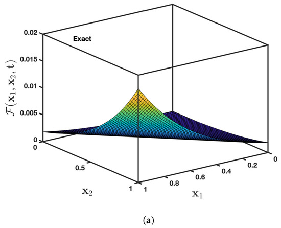
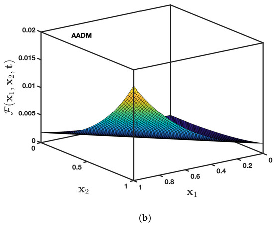
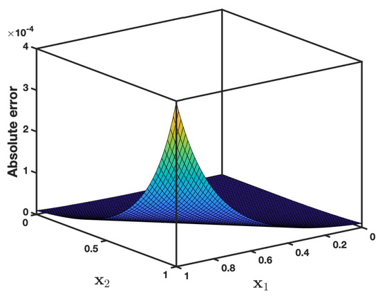
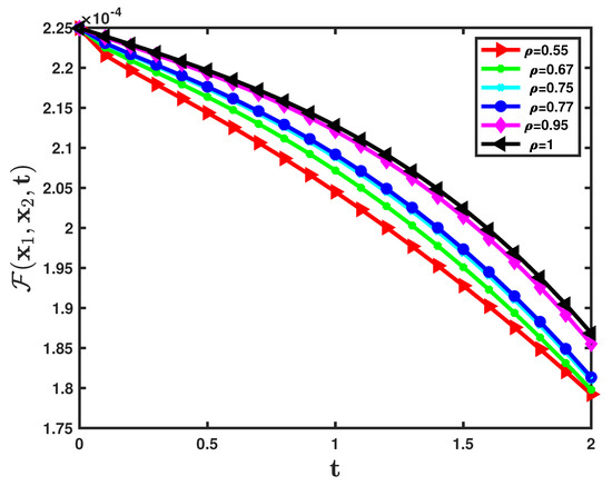
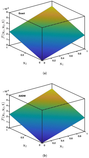
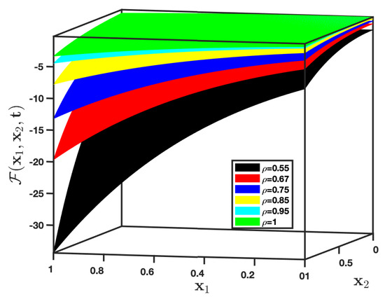
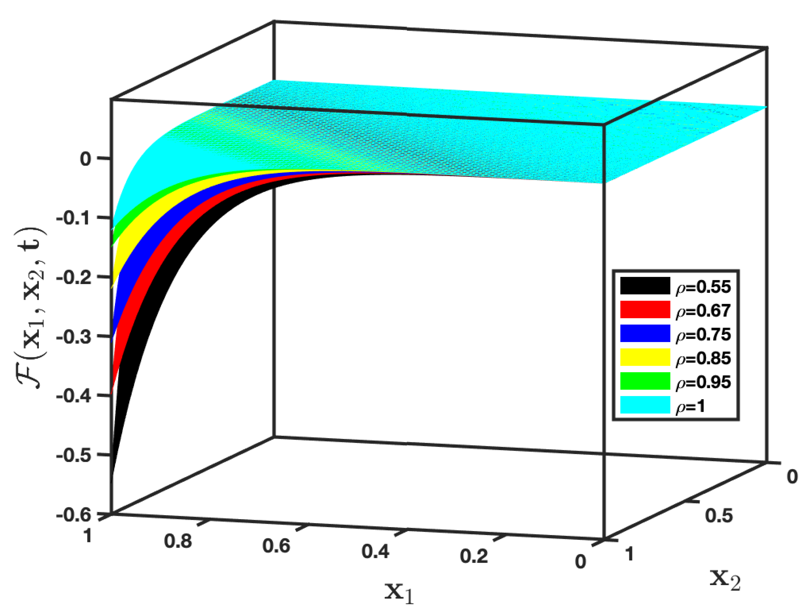
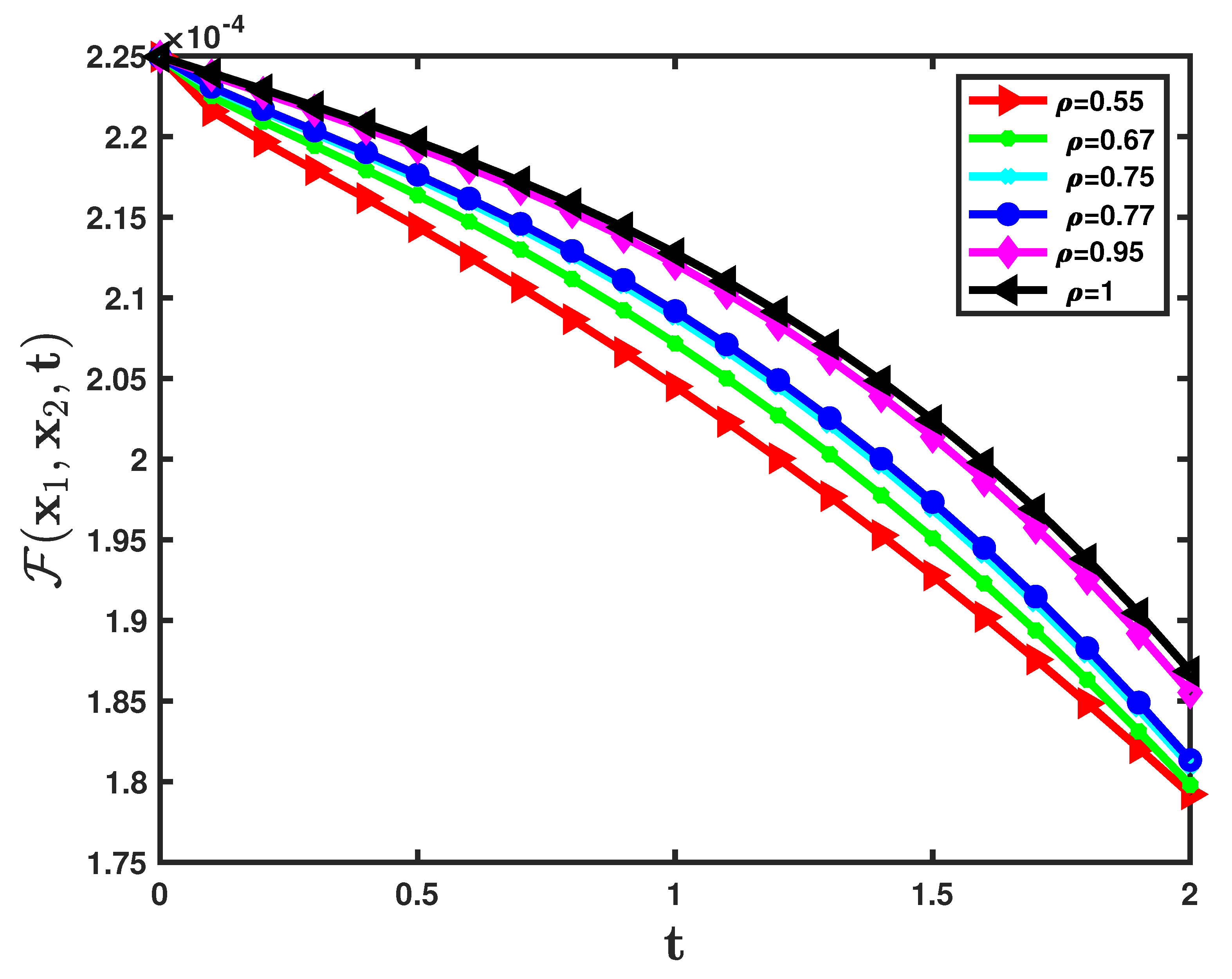
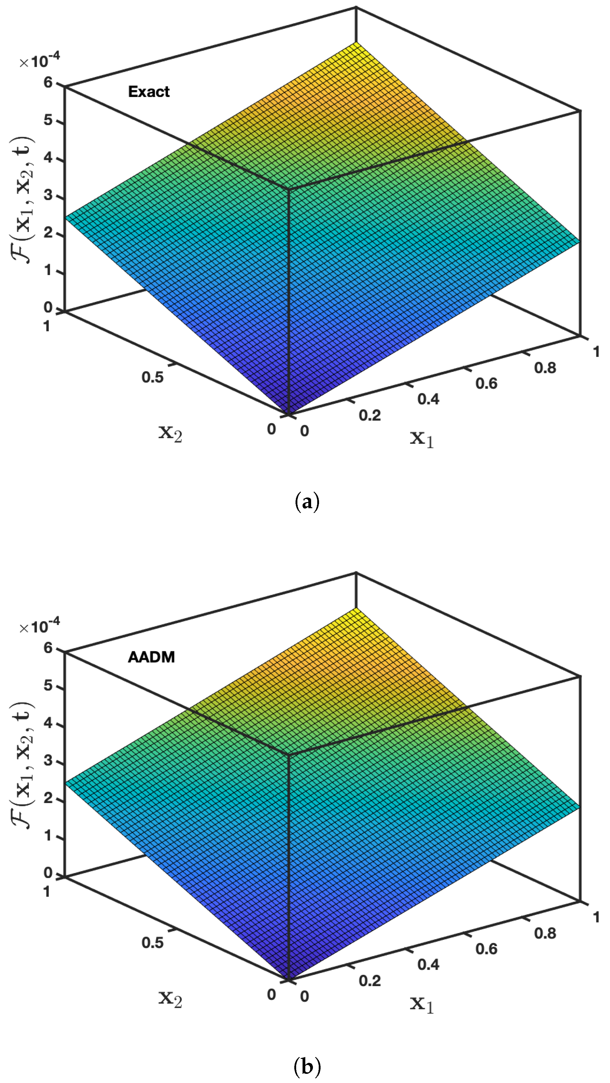
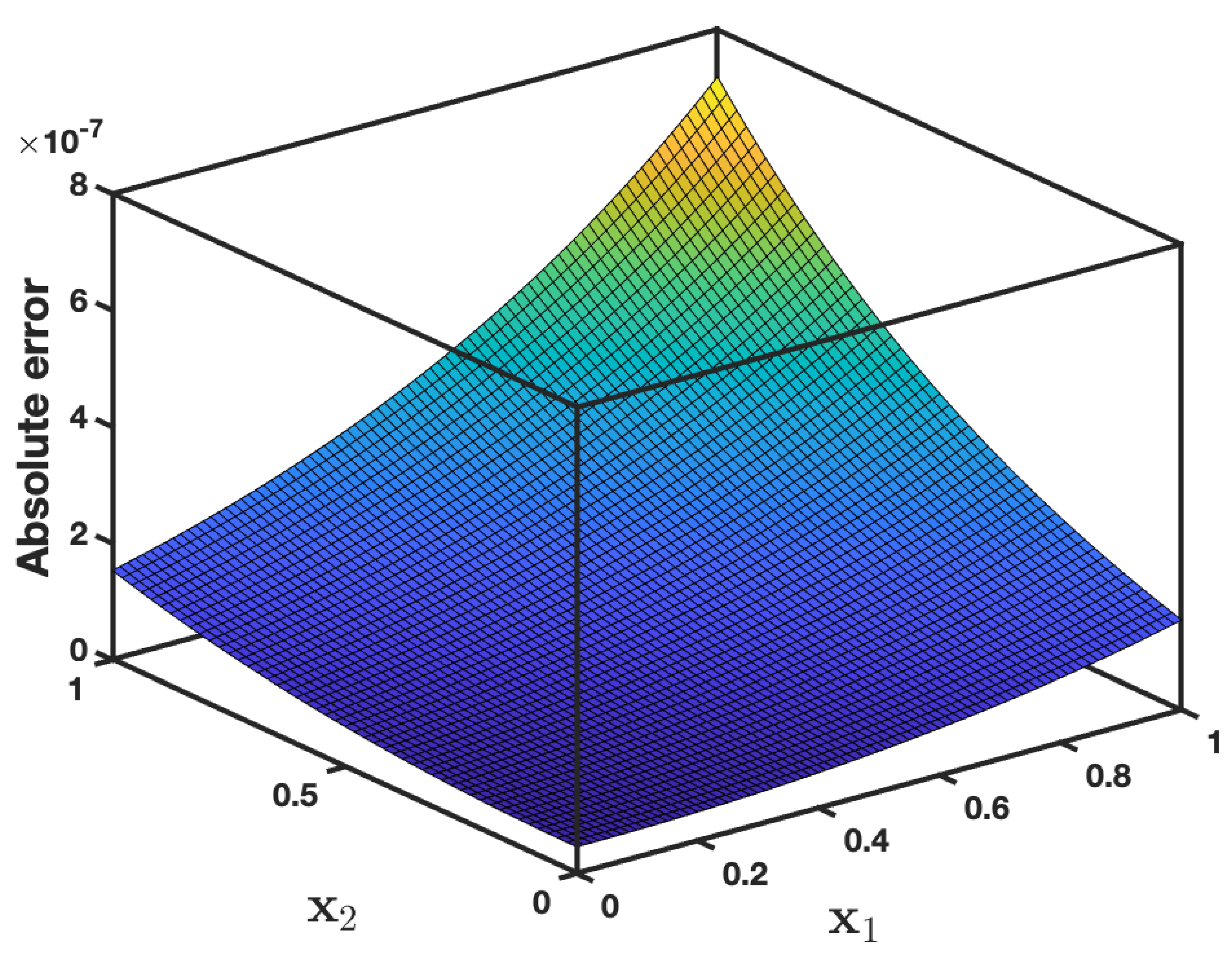
Table 1 and Table 2 demonstrates the exact AADM solution and the absolute error $E_{abs}=\parallel E^{exact}-E^{approx}\parallel$ for Problem 1. Figure 1 represents the comparison between the exact (left) and the approximate (right) solution, while Figure 2 describes the surface plot of the absolute error of the solution when $\rho =1,$ and $\lambda =0.001$. Figure 3 represents a surface plot of approximate solutions for various fractional orders, $\rho =0.55$, $0.67$, $0.75$, $0.85$, $0.95$, and 1. In addition, Figure 4 addresses approximate solutions for various fractional orders: $\rho =0.55$, $0.67$, $0.75$, $0.77$, $0.95$, and 1 converge very rapidly to exact solutions, implying that approximate solutions are almost similar to exact solutions. As a result, the VIM [41] and HPM [42] demanded the evaluation of the Lagrangian multiplier, but the AADM demanded the evaluation of the Adomian polynomials, which entails less computation algebraic work. By obtaining further expressions of approximate solutions, the reliability of the analysis can be strengthened. □

Table 1. Exact and AADM-approximate solution with absolute error in comparison derived by PIA and RPSM for Problem 1 at $\lambda =0.001,$ $\rho =1$.

${\mathit{x}}_1$	${\mathit{x}}_2$	t	AADM Solution	Exact Solution	PIA [37] Error	RPSM [37] Error	AADM Error
0.1	0.1	0.2	5.3966 × ${10}^{-5}$	5.39388 × ${10}^{-5}$	3.85217 × ${10}^{-7}$	3.85217 × ${10}^{-7}$	2.71884 × ${10}^{-8}$
0.1	0.1	0.3	5.39248 × ${10}^{-5}$	5.38841 × ${10}^{-5}$	5.75911 × ${10}^{-7}$	5.75912 × ${10}^{-7}$	4.07394 × ${10}^{-8}$
0.1	0.1	0.4	5.38837 × ${10}^{-5}$	5.38294 × ${10}^{-5}$	7.65359 × ${10}^{-7}$	7.65352 × ${10}^{-7}$	5.42615 × ${10}^{-8}$
0.6	0.6	0.2	3.02967 × ${10}^{-3}$	3.03651 × ${10}^{-3}$	4.66337 × ${10}^{-5}$	4.66389 × ${10}^{-5}$	6.83433 × ${10}^{-6}$
0.6	0.6	0.3	3.02553 × ${10}^{-3}$	3.03578 × ${10}^{-3}$	6.86056 × ${10}^{-5}$	6.86314 × ${10}^{-5}$	1.02517 × ${10}^{-5}$
0.6	0.6	0.4	3.02138 × ${10}^{-3}$	3.03505 × ${10}^{-3}$	8.98263 × ${10}^{-5}$	8.99046 × ${10}^{-5}$	1.36692 × ${10}^{-5}$
0.9	0.9	0.2	1.14455 × ${10}^{-2}$	1.15370 × ${10}^{-2}$	5.12131 × ${10}^{-4}$	5.14241 × ${10}^{-4}$	9.14704 × ${10}^{-5}$
0.9	0. 9	0.3	1.13973 × ${10}^{-2}$	1.15345 × ${10}^{-2}$	7.38186 × ${10}^{-4}$	7.48450 × ${10}^{-4}$	1.37206 × ${10}^{-4}$
0.9	0.9	0.4	1.13492 × ${10}^{-2}$	1.15321 × ${10}^{-2}$	9.57942 × ${10}^{-4}$	9.89139 × ${10}^{-4}$	1.82943 × ${10}^{-4}$

Table 2. Exact and AADM-approximate solution in comparison with PIA and RPSM for Problem 1 at $\lambda =0.001$ for fractional-order $\rho =0.67$ and $\rho =0.75$.

${\mathit{x}}_1/{\mathit{x}}_2$	t	AADM Solution	PIA [37]	RPSM [37]	AADM Solution	PIA [37]	RPSM [37]
0.1	0.2	5.39424 × ${10}^{-5}$	5.31854 × ${10}^{-5}$	5.31244 × ${10}^{-5}$	5.3953 × ${10}^{-5}$	5.32747 × ${10}^{-5}$	5.32479 × ${10}^{-5}$
0.1	0.3	5.39094 × ${10}^{-5}$	5.28631 × ${10}^{-5}$	5.28410 × ${10}^{-5}$	5.39191 × ${10}^{-5}$	5.29757 × ${10}^{-5}$	5.29675 × ${10}^{-5}$
0.1	0.4	5.38798 × ${10}^{-5}$	5.25777 × ${10}^{-5}$	5.25897 × ${10}^{-5}$	5.38881 × ${10}^{-5}$	5.27039 × ${10}^{-5}$	5.27119 × ${10}^{-5}$
0.6	0.2	3.02730 × ${10}^{-3}$	2.95493 × ${10}^{-3}$	2.95185 × ${10}^{-3}$	3.02837 × ${10}^{-3}$	2.96356 × ${10}^{-3}$	2.96251 × ${10}^{-3}$
0.6	0.3	3.02397 × ${10}^{-3}$	2.92662 × ${10}^{-3}$	2.92709 × ${10}^{-3}$	3.02496 × ${10}^{-3}$	2.93717 × ${10}^{-3}$	2.93780 × ${10}^{-3}$
0.6	0.4	3.02099 × ${10}^{-3}$	2.90307 × ${10}^{-3}$	2.90522 × ${10}^{-3}$	3.02182 × ${10}^{-3}$	2.91448 × ${10}^{-3}$	2.91561 × ${10}^{-3}$
0.9	0.2	1.14179 × ${10}^{-2}$	1.06822 × ${10}^{-2}$	1.05522 × ${10}^{-2}$	1.14303 × ${10}^{-2}$	1.07716 × ${10}^{-2}$	2.91561 × ${10}^{-2}$
0.9	0.3	1.13792 × ${10}^{-2}$	1.04487 × ${10}^{-2}$	1.01199 × ${10}^{-2}$	1.13907 × ${10}^{-2}$	1.05488 × ${10}^{-2}$	1.03695 × ${10}^{-2}$
0.9	0.4	1.13447 × ${10}^{-2}$	9.02777 × ${10}^{-2}$	9.60606 × ${10}^{-2}$	1.13543 × ${10}^{-2}$	1.03736 × ${10}^{-2}$	9.96743 × ${10}^{-2}$

Figure 1. Numerical behaviours for Problem 1 established by the integer-order (a) ρ = 1 and (b) the AADM at t = 0.1 with the parameters λ = 0.001 for various values of x₁, and x₂.

Figure 2. The absolute-error of solution of Problem 1 at $\mathbf{t}=0.1$ with the parameters $\rho =1,$ $\lambda =0.001$.

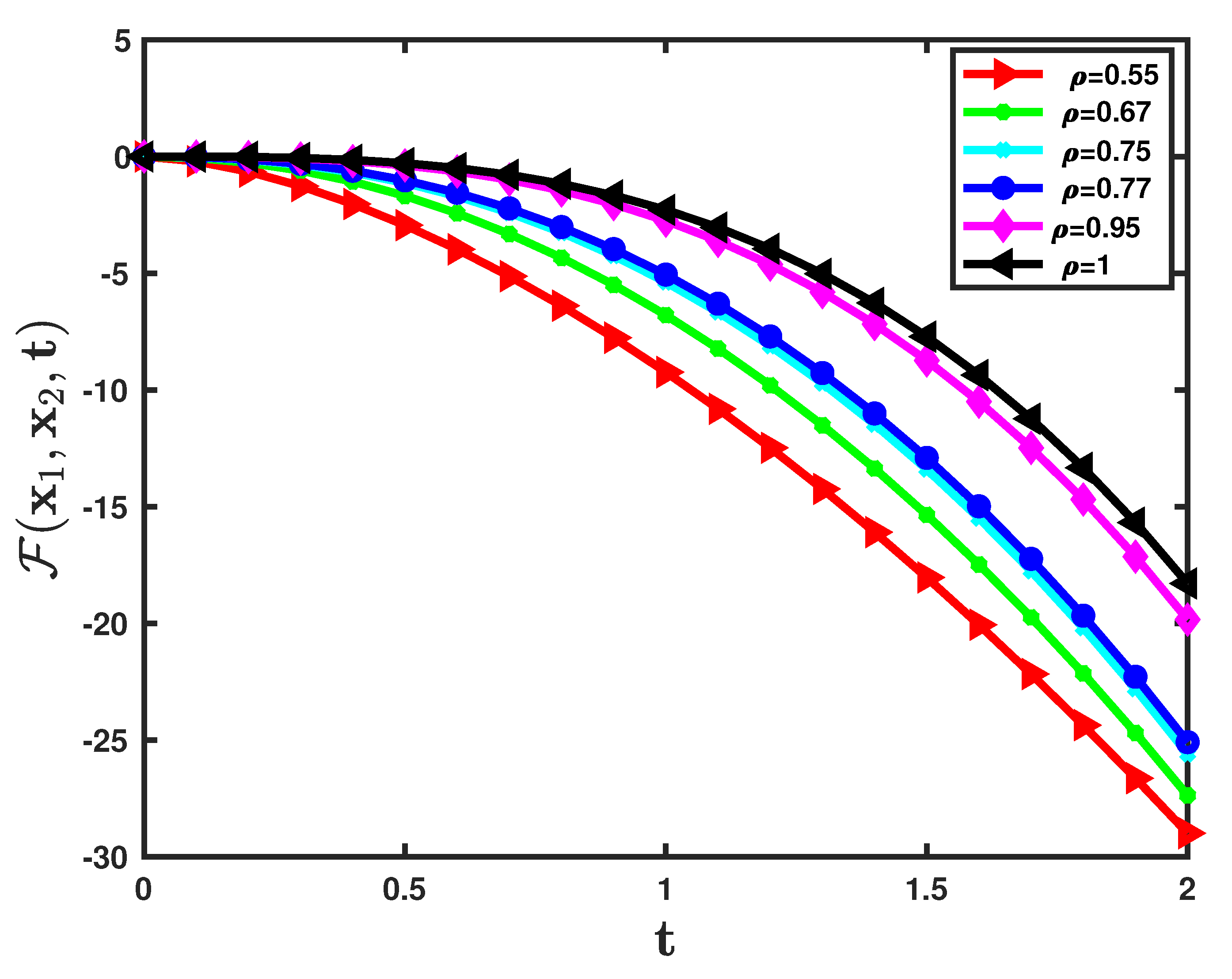
Figure 3. The approximate-analytical AADM solution $\mathcal{F}({\mathbf{x}}_1,{\mathbf{x}}_2,\mathbf{t})$ of Problem 1 for $\rho =$ 0.55, 0.67, 0.75, 0.85, 0.95, and 1 with the parameter $\lambda =0.001$.

Figure 4. Convergence at various values of $\rho$ and $\mathbf{t}$ for Equation (21) at ${\mathbf{x}}_1=0.2,$${\mathbf{x}}_2=0.2$ with the parameter $\lambda =0.001$.

Problem 2.

Assume the following time-dependent fractional-order Zakharov–Kuznetsov equation [41,42]:

$$\begin{array}{c}\hfill {\mathcal{D}}_{\mathbf{t}}^{\rho }\mathcal{F}+\frac{\partial {\mathcal{F}}^3}{\partial {\mathbf{x}}_1}+2\left[\frac{\partial }{\partial {\mathbf{x}}_1}\left(\frac{{\partial }^2{\mathcal{F}}^3}{\partial {\mathbf{x}}_2^2}\right)+\frac{{\partial }^3{\mathcal{F}}^3}{\partial {\mathbf{x}}_1^3}\right]=0,0<\rho \le 1\end{array}$$

(32)

subject to the initial condition

$$\begin{array}{c}\hfill \mathcal{F}({\mathbf{x}}_1,{\mathbf{x}}_2,0)=\frac{3}{2}\lambda sinh\left[\frac{1}{6}({\mathbf{x}}_1+{\mathbf{x}}_2)\right],\end{array}$$

(33)

where λ is an arbitrary constant.

Proof. 

Applying the AT on both sides of (32), we find

$$\begin{array}{ccc}\hfill & & \mathbb{A}\left[\frac{{\partial }^{\rho }\mathcal{F}}{\partial {\mathbf{t}}^{\rho }}\right]=-\mathbb{A}\left[\frac{\partial {\mathcal{F}}^3}{\partial {\mathbf{x}}_1}+2\left[\frac{\partial }{\partial {\mathbf{x}}_1}\left(\frac{{\partial }^2{\mathcal{F}}^3}{\partial {\mathbf{x}}_2^2}\right)+\frac{{\partial }^3{\mathcal{F}}^3}{\partial {\mathbf{x}}_1^3}\right]\right],\hfill \\ & & {\omega }^{\rho }\mathbb{A}\left[\mathcal{F}({\mathbf{x}}_1,{\mathbf{x}}_2,\mathbf{t})\right]-\sum _{\kappa =0}^{n_1-1}\frac{{\mathcal{F}}^{\left(\kappa \right)}\left(0\right)}{{\omega }^{2-\rho +\kappa }}=-\mathbb{A}\left[\frac{\partial {\mathcal{F}}^3}{\partial {\mathbf{x}}_1}+2\left[\frac{\partial }{\partial {\mathbf{x}}_1}\left(\frac{{\partial }^2{\mathcal{F}}^3}{\partial {\mathbf{x}}_2^2}\right)+\frac{{\partial }^3{\mathcal{F}}^3}{\partial {\mathbf{x}}_1^3}\right]\right].\hfill \end{array}$$

(34)

Employing the inverse AT, we have

$$\begin{array}{c}\hfill \mathcal{F}({\mathbf{x}}_1,{\mathbf{x}}_2,\mathbf{t})={\mathbb{A}}^{-1}\left[\frac{1}{{\omega }^{\rho }}\sum _{\kappa =0}^{n_1-1}\frac{{\mathcal{F}}^{\left(\kappa \right)}\left(0\right)}{{\omega }^{2-\rho +\kappa }}-\frac{1}{{\omega }^{\rho }}\mathbb{A}\left[\frac{\partial {\mathcal{F}}^3}{\partial {\mathbf{x}}_1}+2\left[\frac{\partial }{\partial {\mathbf{x}}_1}\left(\frac{{\partial }^2{\mathcal{F}}^3}{\partial {\mathbf{x}}_2^2}\right)+\frac{{\partial }^3{\mathcal{F}}^3}{\partial {\mathbf{x}}_1^3}\right]\right]\right].\end{array}$$

(35)

It follows that

$$\begin{array}{ccc}& & \mathcal{F}({\mathbf{x}}_1,{\mathbf{x}}_2,\mathbf{t})={\mathbb{A}}^{-1}\left[\frac{\mathcal{F}({\mathbf{x}}_1,{\mathbf{x}}_2,0)}{{\omega }^2}\right]-{\mathbb{A}}^{-1}\left[\frac{1}{{\omega }^{\rho }}\mathbb{A}\left[\frac{\partial {\mathcal{F}}^3}{\partial {\mathbf{x}}_1}+2\left[\frac{\partial }{\partial {\mathbf{x}}_1}\left(\frac{{\partial }^2{\mathcal{F}}^3}{\partial {\mathbf{x}}_2^2}\right)+\frac{{\partial }^3{\mathcal{F}}^3}{\partial {\mathbf{x}}_1^3}\right]\right]\right],\hfill \\ & & \mathcal{F}({\mathbf{x}}_1,{\mathbf{x}}_2,\mathbf{t})={\mathbb{A}}^{-1}\left[\frac{3}{2}\frac{\lambda sinh\left[\frac{1}{6}({\mathbf{x}}_1+{\mathbf{x}}_2)\right]}{{\omega }^2}\right]-{\mathbb{A}}^{-1}\left[\frac{1}{{\omega }^{\rho }}\mathbb{A}\left[\frac{\partial {\mathcal{F}}^3}{\partial {\mathbf{x}}_1}+2\left[\frac{\partial }{\partial {\mathbf{x}}_1}\left(\frac{{\partial }^2{\mathcal{F}}^3}{\partial {\mathbf{x}}_2^2}\right)+\frac{{\partial }^3{\mathcal{F}}^3}{\partial {\mathbf{x}}_1^3}\right]\right]\right].\hfill \end{array}$$

(36)

Utilizing the Adomian decomposition method, we obtain

$$\begin{array}{c}\hfill \sum _{j=0}^{\infty }{\mathcal{F}}_j({\mathbf{x}}_1,{\mathbf{x}}_2,\mathbf{t})=\frac{3}{2}\lambda sinh\left[\frac{1}{6}({\mathbf{x}}_1+{\mathbf{x}}_2)\right]-{\mathbb{A}}^{-1}\left[\frac{1}{{\omega }^{\rho }}\mathbb{A}\left[\mathcal{N}{\left(\mathcal{F}\right)}_{{\mathbf{x}}_1}+\frac{1}{8}\left[\mathcal{N}{\left(\mathcal{F}\right)}_{{\mathbf{x}}_1{\mathbf{x}}_1{\mathbf{x}}_1}+\mathcal{N}{\left(\mathcal{F}\right)}_{{\mathbf{x}}_1{\mathbf{x}}_2{\mathbf{x}}_2}\right]\right]\right],\end{array}$$

(37)

where $\mathcal{N}\left(\mathcal{F}\right)$ is the He’s polynomial describing a nonlinear term appearing in the abovementioned equations.

$$\begin{array}{c}\hfill \mathcal{N}\left(\mathcal{F}\right)={\mathcal{F}}^3=\sum _{j=0}^{\infty }{\mathcal{G}}_j\left(\mathcal{F}\right).\end{array}$$

(38)

First a few He’s polynomials are presented as follows:

$$\begin{array}{ccc}\hfill {\mathcal{G}}_0& & ={\mathcal{F}}_0^3,\hfill \\ \hfill {\mathcal{G}}_1& & =3{\mathcal{F}}_0^2{\mathcal{F}}_1,\hfill \\ \hfill {\mathcal{G}}_2& & =3{\mathcal{F}}_0^2{\mathcal{F}}_2+3{\mathcal{F}}_0^2{\mathcal{F}}_1^2,\hfill \\ \hfill {\mathcal{F}}_0({\mathbf{x}}_1,{\mathbf{x}}_2,\mathbf{t})& & =\frac{3}{2}\lambda sinh\left[\frac{1}{6}({\mathbf{x}}_1+{\mathbf{x}}_2)\right],\hfill \\ \hfill {\mathcal{F}}_{j+1}({\mathbf{x}}_1,{\mathbf{x}}_2,\mathbf{t})& & =-{\mathbb{A}}^{-1}[\frac{1}{{\omega }^{\rho }}\mathbb{A}\left[{\left(\sum _{j=0}^{\infty }{\mathcal{G}}_j\left(\mathcal{F}\right)\right)}_{{\mathbf{x}}_1}+2{\left(\sum _{j=0}^{\infty }{\mathcal{G}}_j\left(\mathcal{F}\right)\right)}_{{\mathbf{x}}_1{\mathbf{x}}_1{\mathbf{x}}_1}+2{\left(\sum _{j=0}^{\infty }{\mathcal{G}}_j\left(\mathcal{F}\right)\right)}_{{\mathbf{x}}_1{\mathbf{x}}_2{\mathbf{x}}_2}\right],\hfill \end{array}$$

for $j=0,1,2,...$

$$\begin{array}{ccc}\hfill {\mathcal{F}}_1({\mathbf{x}}_1,{\mathbf{x}}_2,\mathbf{t})& & =-{\mathbb{A}}^{-1}\left[\frac{1}{{\omega }^{\rho }}\mathbb{A}\left[{\left({\mathcal{F}}_0^3\right)}_{{\mathbf{x}}_1}+2{\left({\mathcal{F}}_0^3\right)}_{{\mathbf{x}}_1{\mathbf{x}}_1{\mathbf{x}}_1}+2{\left({\mathcal{F}}_0^3\right)}_{{\mathbf{x}}_1{\mathbf{x}}_2{\mathbf{x}}_2}\right]\right]\hfill \\ & & =\left(-3{\lambda }^3{sinh}^2\left[\frac{1}{6}({\mathbf{x}}_1+{\mathbf{x}}_2)\right]cosh\left[\frac{1}{6}({\mathbf{x}}_1+{\mathbf{x}}_2)\right]+\frac{3}{8}{\lambda }^3{cosh}^3\left[\frac{1}{6}({\mathbf{x}}_1+{\mathbf{x}}_2)\right]\right){\mathbb{A}}^{-1}\left(\frac{1}{{\omega }^{\rho +2}}\right)\hfill \\ & & =\left(-3{\lambda }^3{sinh}^2\left[\frac{1}{6}({\mathbf{x}}_1+{\mathbf{x}}_2)\right]cosh\left[\frac{1}{6}({\mathbf{x}}_1+{\mathbf{x}}_2)\right]+\frac{3}{8}{\lambda }^3{cosh}^3\left[\frac{1}{6}({\mathbf{x}}_1+{\mathbf{x}}_2)\right]\right)\frac{{\mathbf{t}}^{\rho }}{\Gamma (\rho +1)}.\hfill \end{array}$$

Accordingly, we can derive the remaining terms as follows:

$$\begin{array}{ccc}\hfill {\mathcal{F}}_2({\mathbf{x}}_1,{\mathbf{x}}_2,\mathbf{t})& & =-{\mathbb{A}}^{-1}\left[\frac{1}{{\omega }^{\rho }}\mathbb{A}\left[{\left(3{\mathcal{F}}_0^2{\mathcal{F}}_1\right)}_{{\mathbf{x}}_1}+2{\left(3{\mathcal{F}}_0^2{\mathcal{F}}_1\right)}_{{\mathbf{x}}_1{\mathbf{x}}_1{\mathbf{x}}_1}+2{\left(3{\mathcal{F}}_0^2{\mathcal{F}}_1\right)}_{{\mathbf{x}}_1{\mathbf{x}}_2{\mathbf{x}}_2}\right]\right]\hfill \\ & & =\frac{3}{32}{\lambda }^{5}sinh\left[\frac{1}{6}({\mathbf{x}}_1+{\mathbf{x}}_2)\right]\left[765{cosh}^4\left[\frac{1}{6}({\mathbf{x}}_1+{\mathbf{x}}_2)\right]-729{cosh}^2\left[\frac{1}{6}({\mathbf{x}}_1+{\mathbf{x}}_2)\right]+91\right]\frac{{\mathbf{t}}^{2\rho }}{\Gamma (2\rho +1)},\hfill \end{array}$$

$$\begin{array}{ccc}\hfill {\mathcal{F}}_3({\mathbf{x}}_1,{\mathbf{x}}_2,\mathbf{t})& & =-{\mathbb{A}}^{-1}\left[\frac{1}{{\omega }^{\rho }}\mathbb{A}\left[{(3{\mathcal{F}}_0^2{\mathcal{F}}_2+3{\mathcal{F}}_0^2{\mathcal{F}}_1^2)}_{{\mathbf{x}}_1}+2{(3{\mathcal{F}}_0^2{\mathcal{F}}_2+3{\mathcal{F}}_0^2{\mathcal{F}}_1^2)}_{{\mathbf{x}}_1{\mathbf{x}}_1{\mathbf{x}}_1}+2{(3{\mathcal{F}}_0^2{\mathcal{F}}_2+3{\mathcal{F}}_0^2{\mathcal{F}}_1^2)}_{{\mathbf{x}}_1{\mathbf{x}}_2{\mathbf{x}}_2}\right]\right]\hfill \\ & & =-\frac{3}{128}cosh\left[\frac{1}{6}({\mathbf{x}}_1+{\mathbf{x}}_2)\right][171,738{cosh}^6\left[\frac{1}{6}({\mathbf{x}}_1+{\mathbf{x}}_2)\right]-349,884{cosh}^4\left[\frac{1}{6}({\mathbf{x}}_1+{\mathbf{x}}_2)\right]\hfill \\ & & +215,496{cosh}^2\left[\frac{1}{6}({\mathbf{x}}_1+{\mathbf{x}}_2)\right]-36,907]\frac{{\mathbf{t}}^{3\rho }}{\Gamma (3\rho +1)}.\hfill \end{array}$$

The approximate analytical AADM solution is

$$\begin{array}{ccc}\hfill \mathcal{F}({\mathbf{x}}_1,{\mathbf{x}}_2,\mathbf{t})& & ={\mathcal{F}}_0({\mathbf{x}}_1,{\mathbf{x}}_2,\mathbf{t})+{\mathcal{F}}_1({\mathbf{x}}_1,{\mathbf{x}}_2,\mathbf{t})+{\mathcal{F}}_2({\mathbf{x}}_1,{\mathbf{x}}_2,\mathbf{t})+{\mathcal{F}}_3({\mathbf{x}}_1,{\mathbf{x}}_2,\mathbf{t})+...,\hfill \\ \hfill \mathcal{F}({\mathbf{x}}_1,{\mathbf{x}}_2,\mathbf{t})& & =\frac{3}{2}\lambda sinh\left[\frac{1}{6}({\mathbf{x}}_1+{\mathbf{x}}_2)\right]\hfill \\ & & -\left(3{\lambda }^3{sinh}^2\left[\frac{1}{6}({\mathbf{x}}_1+{\mathbf{x}}_2)\right]cosh\left[\frac{1}{6}({\mathbf{x}}_1+{\mathbf{x}}_2)\right]+\frac{3}{8}{\lambda }^3{cosh}^3\left[\frac{1}{6}({\mathbf{x}}_1+{\mathbf{x}}_2)\right]\right)\frac{{\mathbf{t}}^{\rho }}{\Gamma (\rho +1)}\hfill \\ & & +\frac{3}{32}{\lambda }^{5}sinh\left[\frac{1}{6}({\mathbf{x}}_1+{\mathbf{x}}_2)\right]\left[765{cosh}^4\left[\frac{1}{6}({\mathbf{x}}_1+{\mathbf{x}}_2)\right]-729{cosh}^2\left[\frac{1}{6}({\mathbf{x}}_1+{\mathbf{x}}_2)\right]+91\right]\frac{{\mathbf{t}}^{2\rho }}{\Gamma (2\rho +1)}\hfill \\ & & -\frac{3}{128}cosh\left[\frac{1}{6}({\mathbf{x}}_1+{\mathbf{x}}_2)\right][171,738{cosh}^6\left[\frac{1}{6}({\mathbf{x}}_1+{\mathbf{x}}_2)\right]-349,884{cosh}^4\left[\frac{1}{6}({\mathbf{x}}_1+{\mathbf{x}}_2)\right]\hfill \\ & & +215,496{cosh}^2\left[\frac{1}{6}({\mathbf{x}}_1+{\mathbf{x}}_2)\right]-36,907]\frac{{\mathbf{t}}^{3\rho }}{\Gamma (3\rho +1)}+....\hfill \end{array}$$

(39)

The exact solution for $\rho =1$ is presented by

$$\begin{array}{c}\hfill \mathcal{F}({\mathbf{x}}_1,{\mathbf{x}}_2,\mathbf{t})=\frac{3}{2}\lambda sinh\left[\frac{1}{6}({\mathbf{x}}_1+{\mathbf{x}}_2-\lambda \mathbf{t})\right].\end{array}$$

(40)

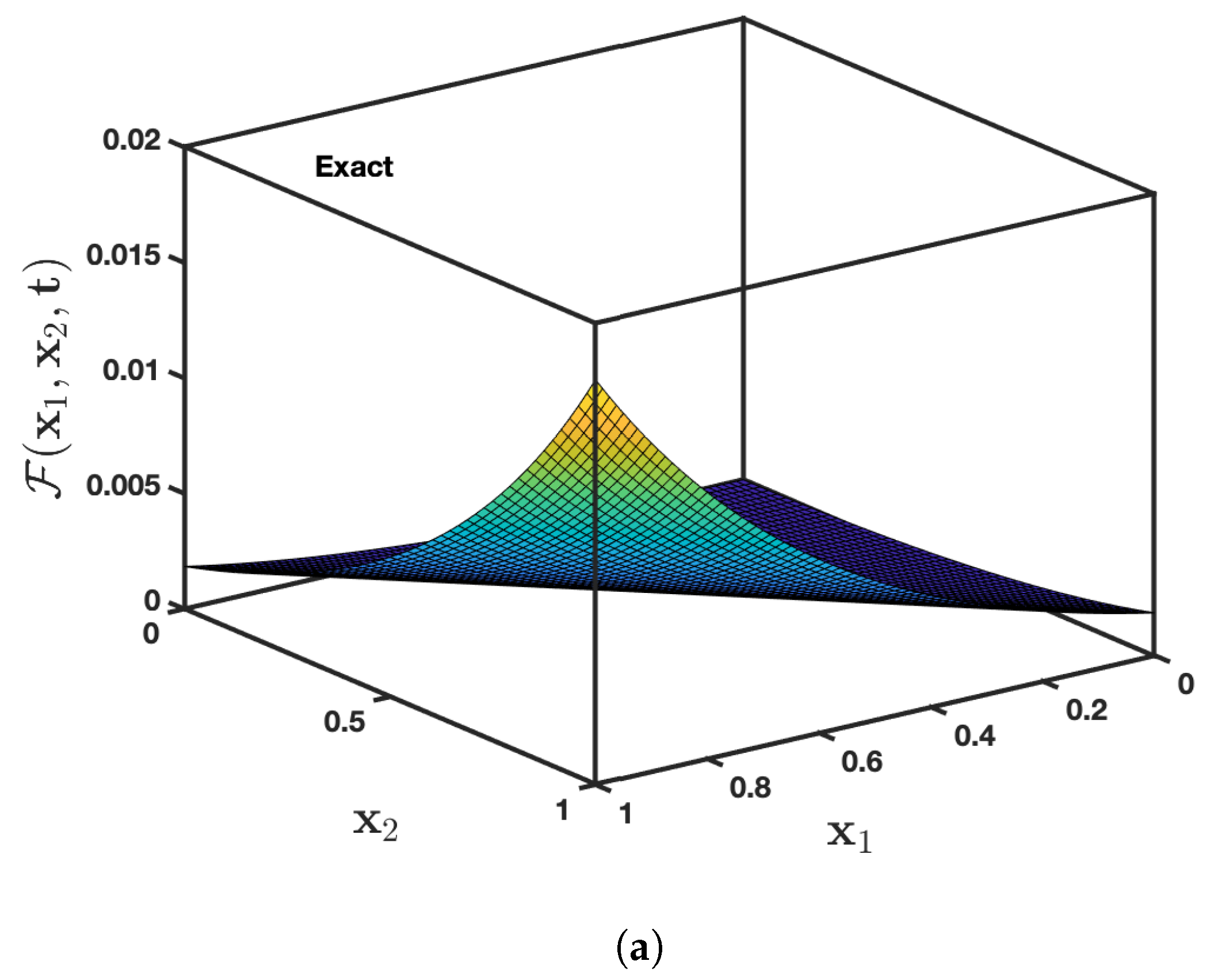
Table 3 and Table 4 demonstrates the exact AADM solution and the absolute error $E_{abs}=\parallel E^{exact}-E^{approx}\parallel$ for Problem 2. Figure 5 represents the comparison between the exact (left) and the approximate (right) solution, while Figure 6 describes the surface plot of the absolute error of the solution when $\rho =1,$ and $\lambda =0.001$. Figure 7 represents a surface plot of approximate solutions for various fractional orders $\rho =0.55$, $0.67$, $0.75$, $0.85$, $0.95$, and 1. In addition, Figure 8 addresses approximate solutions for various fractional orders: $\rho =0.55$, $0.67$, $0.75$, $0.77$, $0.95$, and 1 converge very rapidly to exact solutions, implying that approximate solutions are almost similar to exact solutions. As a comparison, the VIM [41] and HPM [42] necessitated the evaluation of the Lagrangian multiplier, but the AADM required the evaluation of the Adomian polynomials, which involved less algebraic computation. By obtaining further expressions of approximate solutions, the reliability of the analysis can be strengthened. □

Table 3. AADM and exact solution with absolute error solution in comparison with the solution derived by VIM for Problem 2 at $\lambda =0.001$ and $\alpha =1$.

${\mathit{x}}_1$	${\mathit{x}}_2$	t	AADM Solution	Exact Solution	VIM [41] Error	AADM Error
0.1	0.1	0.2	5.00092 × ${10}^{-5}$	4.99592 × ${10}^{-5}$	5.00091 × ${10}^{-5}$	4.99519 × ${10}^{-8}$
0.1	0.1	0.3	5.00091 × ${10}^{-5}$	4.99342 × ${10}^{-5}$	5.00091 × ${10}^{-5}$	7.49278 × ${10}^{-8}$
0.1	0.1	0.4	5.00091 × ${10}^{-5}$	4.99092 × ${10}^{-5}$	5.00091 × ${10}^{-5}$	9.99037 × ${10}^{-8}$
0.6	0.6	0.2	3.02004 × ${10}^{-4}$	3.01953 × ${10}^{-4}$	3.02003 × ${10}^{-4}$	5.08987 × ${10}^{-8}$
0.6	0.6	0.3	3.02004 × ${10}^{-4}$	3.01927 × ${10}^{-4}$	3.02003 × ${10}^{-4}$	7.63479 × ${10}^{-8}$
0.6	0.6	0.4	3.02004 × ${10}^{-4}$	3.01902 × ${10}^{-4}$	3.02003 × ${10}^{-4}$	1.01797 × ${10}^{-7}$
0.9	0.9	0.2	4.5678 × ${10}^{-4}$	4.56728 × ${10}^{-4}$	4.56780 × ${10}^{-4}$	5.21227 × ${10}^{-8}$
0.9	0. 9	0.3	4.5678 × ${10}^{-4}$	4.56702 × ${10}^{-4}$	4.56780 × ${10}^{-4}$	7.81839 × ${10}^{-8}$
0.9	0.9	0.4	4.5678 × ${10}^{-4}$	4.56676 × ${10}^{-4}$	4.56780 × ${10}^{-4}$	1.04245 × ${10}^{-7}$

Table 4. AADM solution in comparison derived by VIM for Problem 2 at $\lambda =0.001$ and different fractional-orders $\rho =0.67$ and $0.75$.

${\mathit{x}}_1/{\mathit{x}}_2$	t	AADM for $\mathit{\rho }=0.67$	VIM [41] for $\mathit{\rho }=0.67$	AADM for $\mathit{\rho }=0.75$	VIM [41] for $\mathit{\rho }=0.75$
0.1	0.2	5.00091 × ${10}^{-5}$	5.00091 × ${10}^{-5}$	5.00091 × ${10}^{-5}$	5.00091 × ${10}^{-5}$
0.1	0.3	5.00091 × ${10}^{-5}$	5.00090 × ${10}^{-5}$	5.00091 × ${10}^{-5}$	5.00090 × ${10}^{-5}$
0.1	0.4	5.0009 × ${10}^{-5}$	5.00090 × ${10}^{-5}$	5.00091 × ${10}^{-5}$	5.00090 × ${10}^{-5}$
0.6	0.2	3.02004 × ${10}^{-4}$	3.02003 × ${10}^{-4}$	3.02004 × ${10}^{-4}$	3.02003 × ${10}^{-3}$
0.6	0.3	3.02004 × ${10}^{-4}$	3.02003 × ${10}^{-4}$	3.02004 × ${10}^{-4}$	3.02003 × ${10}^{-3}$
0.6	0.4	3.02004 × ${10}^{-4}$	3.02003 × ${10}^{-4}$	3.02004 × ${10}^{-4}$	3.02003 × ${10}^{-3}$
0.9	0.2	4.5678 × ${10}^{-4}$	4.56780 × ${10}^{-4}$	4.5678 × ${10}^{-4}$	4.5678 × ${10}^{-2}$
0. 9	0.3	4.5678 × ${10}^{-4}$	4.56780 × ${10}^{-4}$	4.5678 × ${10}^{-4}$	4.5678 × ${10}^{-2}$
0.9	0.4	4.5678 × ${10}^{-4}$	4.56780 × ${10}^{-4}$	4.5678 × ${10}^{-4}$	4.5678 × ${10}^{-2}$

Figure 5. Numerical behaviours for Problem 2 established by the integer-order (a) ρ = 1 and (b) the AADM at t = 0.003 with the parameters λ = 0.001 for various values of x₁, and x₂.

Figure 6. The absolute-error of solution of Problem 2 at $\mathbf{t}=0.003$ with the parameters $\rho =1,$ $\lambda =0.001$.

Figure 7. The approximate-analytical AADM solution $\mathcal{F}({\mathbf{x}}_1,{\mathbf{x}}_2,\mathbf{t})$ of Problem 2 for $\rho =$0.55, 0.67, 0.75, 0.85, 0.95, and 1 when the parameter $\lambda =0.001$.

Figure 8. Convergence at various values of $\rho$ and $\mathbf{t}$ for Equation (32) at ${\mathbf{x}}_1=0.2,$ ${\mathbf{x}}_2=0.2$ with the parameter $\lambda =0.001$.

6. Other Aspects of ZKEs

Firstly, considering the fractional order to be 1 and rotating the coordinate axes $(\mathbf{t},\zeta )$ through an angle $\vartheta$, maintaining the $\varpi$-axis stationary, in order to evaluate the temperature dependence of solitary waves in a direction making an angle $\vartheta$ with the $\mathbf{t}$-axis, i.e., with the magnetization and lying in the $(\zeta -\mathbf{t})$ plane, the independent variables are adjusted in the following manner:

$$\begin{array}{c}\hfill {\mathbf{x}}_1=\mathbf{t}sin\vartheta +\zeta cos\vartheta ,{\mathbf{x}}_2=\varpi ,{\mathbf{x}}_3=\mathbf{t}cos\vartheta -\zeta sin\vartheta ,and\mathbf{t}=\tau .\end{array}$$

(41)

Utilizing the aforesaid Scheme (41) in the ZKE (1), yields

$$\begin{array}{ccc}\hfill & & \frac{\partial \mathcal{F}}{\partial \mathbf{t}}+{\eta }_1\mathcal{F}\frac{\partial \mathcal{F}}{\partial {\mathbf{x}}_1}+{\eta }_2\frac{{\partial }^3\mathcal{F}}{\partial {\mathbf{x}}_1^3}+{\eta }_3\mathcal{F}\frac{\partial \mathcal{F}}{\partial {\mathbf{x}}_3}+{\eta }_4\frac{{\partial }^3\mathcal{F}}{\partial {\mathbf{x}}_3^3}+{\eta }_5\frac{{\partial }^3\mathcal{F}}{\partial {\mathbf{x}}_1^2\partial {\mathbf{x}}_3}+{\eta }_6\frac{{\partial }^3\mathcal{F}}{\partial {\mathbf{x}}_1\partial {\mathbf{x}}_3^2}+{\eta }_7\frac{{\partial }^3\mathcal{F}}{\partial {\mathbf{x}}_1\partial {\mathbf{x}}_2^2}\hfill \\ & & +{\eta }_8\frac{{\partial }^3\mathcal{F}}{\partial {\mathbf{x}}_3\partial {\mathbf{x}}_2^2}=0,\hfill \end{array}$$

(42)

where

$$\begin{array}{ccc}\hfill {\eta }_1& & ={\mathbf{A}}_{1}cos\vartheta ,{\eta }_2={\mathbf{A}}_2{cos}^3\vartheta +{\mathbf{A}}_{3}cos\vartheta {sin}^2\vartheta ,{\eta }_3=-{\mathbf{A}}_{1}sin\vartheta ,\hfill \\ \hfill {\eta }_4& & ={\mathbf{A}}_2{sin}^3\vartheta -{\mathbf{A}}_{3}sin\vartheta {cos}^2\vartheta ,{\eta }_5=-3{\mathbf{A}}_{2}sin\vartheta {cos}^2\vartheta -{\mathbf{A}}_3({sin}^2\vartheta -2sin\vartheta {cos}^2\vartheta ),\hfill \\ \hfill {\eta }_6& & =3{\mathbf{A}}_2{sin}^2\vartheta cos\vartheta +{\mathbf{A}}_3({cos}^3\vartheta -2{sin}^2\vartheta cos\vartheta ),{\eta }_7={\mathbf{A}}_{3}cos\vartheta ,{\eta }_8=-{\mathbf{A}}_{3}sin\vartheta .\hfill \end{array}$$

(43)

Now, the steady state solution of the ZKE (42) in the form is investigated as follows:

$$\begin{array}{c}\hfill \mathcal{F}={\mathcal{F}}_0(\Lambda ),\end{array}$$

(44)

where $\Lambda ={\mathbf{x}}_1-\mathcal{U}\mathbf{t},$ whereas $\mathcal{U}$ is a constant velocity normalized to $\mathcal{C}.$ Employing (44) in (42), then, the steady state formulation is represented as

$$\begin{array}{c}\hfill -\mathcal{U}\frac{d{\mathcal{F}}_0}{d\Lambda }+{\eta }_1{\mathcal{F}}_0\frac{d{\mathcal{F}}_0}{d\Lambda }+{\eta }_2\frac{d^3{\mathcal{F}}_0}{d{\Lambda }^3}=0.\end{array}$$

(45)

Utilizing the suitable boundary assumptions, viz., (${\mathcal{F}}_0,{\mathcal{F}}_0^{\prime }$ and ${\mathcal{F}}_0^{\prime \prime }$) tends to 0 when $\Lambda \mapsto \pm \infty ,$ then, the solution of (45) is derived as

$$\begin{array}{c}\hfill {\mathcal{F}}_0(\Lambda )={\mathcal{F}}_{m}sec{h}^2\left(\Lambda /\mathcal{L}\right),\end{array}$$

(46)

where ${\mathcal{F}}_m=3\mathcal{U}/{\eta }_1$ denotes the peak amplitude, and $\mathcal{L}=\sqrt{4{\eta }_2/\mathcal{U}}$ is the width of solitons, respectively. Since the amplitude and width of ion acoustic waves in plasma are influenced by a variety of factors and physical parameters, it is fascinating to quantitatively determine their consequences on plasma carrying superthermality of cold and hot electrons.

Figure 9a,b exhibited symmetric behaviour for positive and negative pressure structures with varied values of density fraction depending on the unperturbed cold electron to fluid ion concentration ratio, in order to see the influence of cold electron superthermality. It is remarkable that with fluctuations in the value of the superthermality of electrons, the wave profile is revealed to be dramatically altered by the superthermality of electrons.

Figure 9. Behaviour of density-fraction (ratio of concentration of cold electrons to ions) (a) changes of positive potential structure: straight curve, dotted-dashed curve, dotted, and dashed curve for density fraction = 0.6, 0.7, 0.8, and 0.9, respectively. (b) Changes of negative potential structure: straight curve, dotted-dashed curve, dotted, and dashed curve for density fraction = 0.2, 0.3, 0.4, and 0.45, respectively.

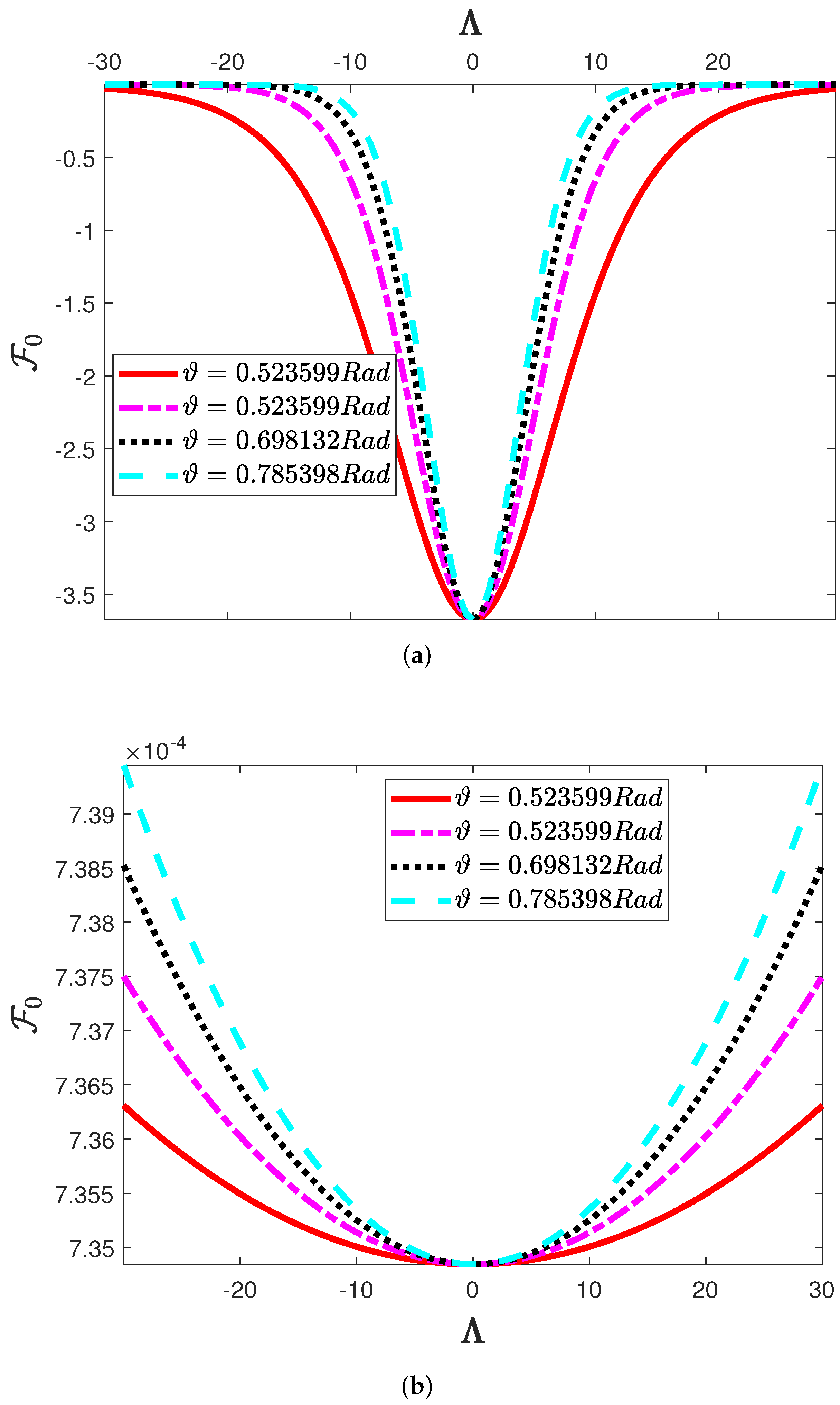
The impact of obliqueness $\vartheta$ on both positive and negative potential is represented in Figure 10a,b. As a result, the increment in obliqueness $\vartheta$ strengthened the amplitude and width, respectively.

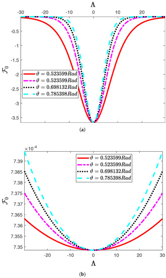
Figure 10. Behaviour of obliqueness-ϑ (a) changes of positive potential structure when density fraction = 0.5: straight curve, dotted-dashed curve, dotted, and dashed curve for ϑ = 30°, 35°, 40°, and 45°, respectively. (b) Changes of negative potential structure when density fraction=0.2: straight curve, dotted-dashed curve, dotted, and dashed curve for density fraction for ϑ = 30°, 35°, 40°, and 45°, respectively.

7. Conclusions

In this study, the AADM was proposed to investigate the time-fractional Zakharov–Kuznetsov equation regulating the nonlinear evolution of ion acoustic waves in a magnetised plasma having cold and hot temperature electrons. For the various physical characteristics, both positive (compressive) and negative (rarefactive) potential structures are generated that are symmetric with respect to origin. The methodology of the suggested technique has been considered to be more effective than other analytical schemes due to its confined number of estimations. The technique is clearly understood by the researchers because it involves implementing the AT explicitly to the projected problem and then adapting the ADM. The inverse Aboodh transform is then employed to derive the approximate solution for the projected problem. To demonstrate the conformity of the developed model and precise solutions to the problems, we have shown 2D and 3D graphs, respectively. The findings acquired by the current report are in excellent accordance with the actual solution of Example 1 and 2 in the paper. Furthermore, the manuscript includes a graph of absolute errors and tabular results which have already been presented and addressed. This demonstrates that the proposed model provided adequate accuracy to the problem solution even though two terms of the series solution were considered. The simulation process reveals that the AADM has achieved an excellent agreement. It may be assumed that the AADM is extremely efficient and easy to implement in determining approximate analytical solutions of several fractional physical and biological models.

References

- Podlubny, I. Fractional Differential Equations; Academic Press: San Diego, CA, USA, 1999. [Google Scholar]
- Hilfer, R. Applications of Fractional Calculus in Physics; Word Scientific: Singapore, 2000. [Google Scholar]
- Kilbas, A.; Srivastava, H.M.; Trujillo, J.J. Theory and Application of Fractional Differential Equations; North Holland Mathematics Studies; Elsevier: Amsterdam, The Netherlands, 2006; Volume 204. [Google Scholar]
- Rahaman, H.; Hasan, M.K.; Ali, A.; Alam, M.S. Implicit methods for numerical solution of singular initial value problems. Appl. Math. Nonliner Scis. 2020, 6, 1–8. [Google Scholar] [CrossRef]
- Aghili, A. Complete solution for the time fractional diffusion problem with mixed boundary conditions by operational method. Appl. Math. Nonliner Sci. 2020, 6, 9–20. [Google Scholar] [CrossRef] [Green Version]
- Magin, R.L. Fractional Calculus in Bioengineering; Begell House Publishers: Danbury, CT, USA, 2006. [Google Scholar]
- Sulaiman, T.A.; Bulut, H.; Baskonus, H.M. On the exact solutions to some system of complex nonlinear models. Appl. Math. Nonliner Sci. 2020, 6, 29–42. [Google Scholar] [CrossRef]
- Samko, S.G.; Kilbas, A.A.; Marichev, O.I. Fractional Integrals and Derivatives: Theory and Applications; Gordon and Breach: Yverdon, Switzerland, 1993. [Google Scholar]
- El-Borhamy, M.; Mosalam, N. On the existence of periodic solution and the transition to chaos of Rayleigh-Duffing equation with application of gyro dynamic. Appl. Math. Nonliner Sci. 2020, 5, 93–108. [Google Scholar] [CrossRef]
- Günerhan, H.; Çelik, E. Analytical and approximate solutions of fractional partial differential-algebraic equations. Appl. Math. Nonlin. Sci. 2020, 5, 109–120. [Google Scholar] [CrossRef]
- Rashid, S.; Khalid, A.; Sultana, S.; Hammouch, Z.; Shah, R.; Alsharif, A.M. A novel analytical view of time-fractional Korteweg–De Vries equations via a new integral transform. Symmetry 2021, 13, 1254. [Google Scholar] [CrossRef]
- Rashid, S.; Kubra, K.T.; Lehre, S.U. Fractional spatial diffusion of a biological population model via a new integral transform in the settings of power and Mittag-Leffler nonsingular kernel. Phy. Scr. 2021, 96. [Google Scholar] [CrossRef]
- Rashid, S.; Kubra, K.T.; Rauf, A.; Chu, Y.-M.; Hamed, Y.S. New numerical approach for time-fractional partial differential equations arising in physical system involving natural decomposition method. Phys. Scr. 2021, 96. [Google Scholar] [CrossRef]
- Debnath, L.; Bhatta, D. Integral Transforms and Their Applications; CRC Press: Boca Raton, FL, USA, 2014. [Google Scholar]
- Aboodh, K.S. The new integral transform Aboodh transform. Glob. J. Pure Appl. Math. 2013, 9, 35–43. [Google Scholar]
- Evirgen, F.; Uçar, S.; Özdemir, N. System analysis of HIV infection model with CD4+T under non-singular kernel derivative. Appl. Math. Nonliner Sci. 2020, 5, 139–146. [Google Scholar] [CrossRef] [Green Version]
- Elzaki, T.M.; Elzaki, S.M. On the ELzaki transform and systems of ordinary differential equations. Glob. J. Pure. Appl. Math. 2011, 7, 113–119. [Google Scholar]
- Watugula, G.K. A new integral transform to solve differential equations and control engineering problems. Int. J. Math. Edu. Sci. Technol. 1993, 24, 409–421. [Google Scholar] [CrossRef]
- Khan, Z.H.; Khan, W.A. Natural transform-properties and applications. NUST J. Eng. Sci. 2008, 1, 127–133. [Google Scholar]
- Maitama, S.; Weidong, Z. New integral transform: Shehu transform a generalization of Sumudu and Laplace transform for solving differential equations. Int. J. Anal. Appl. 2019, 17, 167–190. [Google Scholar]
- Saadeh, R.; Ahmad, Q.; Aliaa, B. A new integral transform: ARA transform and its properties and applications. Symmetry 2020, 12, 925. [Google Scholar] [CrossRef]
- Sharifi, M.; Raesi, B. Vortex theory for two dimensional Boussinesq equations. Appl. Math. Nonliner Sci. 2020, 5, 67–84. [Google Scholar] [CrossRef]
- Rajesh Kanna, M.R.; Pradeep Kumar, R.; Nandappa, S.; Cangul, I.N. On solutions of fractional order telegraph partial differential equation by Crank-Nicholson finite difference method. Appl. Math. Nonliner Sci. 2020, 5, 85–98. [Google Scholar] [CrossRef]
- Daftardar-Gejji, V.; Jafari, H. An iterative method for solving nonlinear functional equations. J. Math. Anal. Appl. 2006, 316, 753–763. [Google Scholar] [CrossRef] [Green Version]
- Daftardar-Gejji, V.; Bhalekar, S. Solving multi-term linear and non-linear diffusion-wave equations of fractional order by Adomian decomposition method. Appl. Math. Comput. 2008, 202, 113. [Google Scholar] [CrossRef]
- Modanli, M.; Akgül, A. On solutions of fractional order Telegraph partial differential equation by Crank-Nicholson finite difference method. Appl. Math. Nonliner Sci. 2020, 5, 163–170. [Google Scholar] [CrossRef] [Green Version]
- Topsakal, M.; Taşcan, F. Exact travelling wave solutions for space-time fractional Klein-Gordon equation and (2+1)-Dimensional time-fractional Zoomeron equation via auxiliary equation method. Appl. Math. Nonliner Sci. 2020, 5, 437–446. [Google Scholar] [CrossRef]
- Bhrawy, A.H.; Abdelkawy, M.A.; Kumar, S.; Johnson, S.; Biswas, A. Solitons and other solutions to quantum Zakharov–Kuznetsov equation in quantum magneto-plasmas. Indian J. Phys. 2013, 87, 455–463. [Google Scholar] [CrossRef]
- Khater, A.H.; Malfliet, W.; Callebaut, D.K.; Kamela, E.S. The tanh method, a simple transformation and exact analytical solutions for nonlinear reaction–diffusion equations. Chaos Solitons Fract. 2002, 14, 513–522. [Google Scholar] [CrossRef]
- Ray, S.S.; Bera, R. Analytical solution of a fractional diffusion equation by Adomian decomposition method. Appl. Math. Comp. 2006, 174, 329–336. [Google Scholar]
- Momani, S.; Odibat, Z. Numerical approach to differential equations of fractional order. J. Comput. Appl. Math. 2007, 207, 96–110. [Google Scholar] [CrossRef] [Green Version]
- Yousef, F.; Alquran, M.; Jaradat, T.; Momani, S.; Baleanu, D. Ternary-fractional differential transform schema: Theory and application. Adv. Differ. Equ. 2019, 2019, 197. [Google Scholar] [CrossRef]
- Hemeda, A.A. Homotopy perturbation method for solving systems of nonlinear coupled equations. Appl. Math. Sci. 2012, 6, 4787–4800. [Google Scholar]
- Marinca, V.; Herisanu, N. The optimal homotopy asymptotic method for solving Blasius equation. Appl. Math. Comput. 2014, 231, 134–139. [Google Scholar] [CrossRef]
- Zayed, E.M.E.; Aljoudi, S. On using the G/G′-expansion method for solving nonlinear partial differential equations in mathematical physics. Commun. Appl. Nonliner Anal. 2010, 17, 49–64. [Google Scholar]
- Li, C.; Zhang, J. Lie symmetry analysis and exact solutions of generalized fractional Zakharov-Kuznetsov equations. Symmetry 2019, 11, 601. [Google Scholar] [CrossRef] [Green Version]
- Şenol, M.; Alquran, M.; Kasmaei, H.D. On the comparison of perturbation-iteration algorithm and residual power series method to solve fractional Zakharov-Kuznetsov equation. Res. Phys. 2018, 9, 321–327. [Google Scholar] [CrossRef]
- Zakharov, V.; Kuznetsov, E. On three-dimensional solitons. Sov. Phys. 1974, 39, 285–288. [Google Scholar]
- Monro, S.; Parkes, E.J. The derivation of a modified Zakharov-Kuznetsov equation and the stability of its solutions. J. Plasma Phys. 1999, 62, 305–317. [Google Scholar] [CrossRef]
- Monro, S.; Parkes, E.J. Stability of solitary-wave solutions to a modified Zakharov-Kuznetsov equation. J. Plasma Phys. 2000, 64, 41126. [Google Scholar] [CrossRef]
- Molliq, R.Y.; Noorani, M.S.M.; Hashim, I.; Ahmad, R.R. Approximate solutions of fractional Zakharov-Kuznetsov equations by VIM. J. Comput. Appl. Math. 2009, 233, 103–108. [Google Scholar] [CrossRef] [Green Version]
- Yildirim, A.; Gulkanat, Y. Analytical approach to fractional Zakharov-Kuznetsov equations by He’s homotopy perturbation method. Commun. Theor. Phys. 2010, 53, 1005. [Google Scholar] [CrossRef]
- Aruldoss, R.; Devi, R.A. Aboodh transform for solving fractional differential equations. Glob. J. Pure Appl. Math. 2020, 16, 145–153. [Google Scholar]
- Aggarwal, S.; Sharma, N.; Chauhan, R. Application of Aboodh transform for solving linear Volterra integro-differential equations of second kind. Int. J. Res. Adv. Technol. 2018, 6, 1186–1190. [Google Scholar]
- Cherif, M.H.; Ziane, D. A new numerical technique for solving systems of nonlinear fractional partial differential equations. Int. J. Anal. Appl. 2017, 15, 188–197. [Google Scholar]
- El-Kalla, I. Convergence of the Adomian method applied to a class of nonlinear integral equations. Appl. Math. Lett. 2008, 21, 372–376. [Google Scholar] [CrossRef] [Green Version]
Publisher’s Note: MDPI stays neutral with regard to jurisdictional claims in published maps and institutional affiliations. |
© 2021 by the authors. Licensee MDPI, Basel, Switzerland. This article is an open access article distributed under the terms and conditions of the Creative Commons Attribution (CC BY) license (https://creativecommons.org/licenses/by/4.0/).