Temporal Behavior of Local Characteristics in Complex Networks with Preferential Attachment-Based Growth

Abstract

The study of temporal behavior of local characteristics in complex growing networks makes it possible to more accurately understand the processes caused by the development of interconnections and links between parts of the complex system that occur as a result of its growth. The spatial position of an element of the system, determined on the basis of connections with its other elements, is constantly changing as the result of these dynamic processes. In this paper, we examine two non-stationary Markov stochastic processes related to the evolution of Barabási–Albert networks: the first describes the dynamics of the degree of a fixed node in the network, and the second is related to the dynamics of the total degree of its neighbors. We evaluate the temporal behavior of some characteristics of the distributions of these two random variables, which are associated with higher-order moments, including their variation, skewness, and kurtosis. The analysis shows that both distributions have a variation coefficient close to 1, positive skewness, and a kurtosis greater than 3. This means that both distributions have huge standard deviations that are of the same order of magnitude as the expected values. Moreover, they are asymmetric with fat right-hand tails.

1. Introduction

Many technological, biological, and social systems can be represented by underlying complex networks. Such networks consist of numerous nodes, and if an interaction between a pair of elements in the system takes place, then it is assumed that the corresponding pair of nodes is connected by a link.

An important exmaple of complex systems of this kind are economic systems, the elements (or nodes) of which are firms or companies, and the links between these elements reflect their economic, informational, or financial interactions. The well-observed effect of the first-mover advantage is that companies that have appeared earlier than others (“first-moving” significant element of the system) usually receive a serious advantage in their development and a larger market segment than firms that entered the market later [1]. The same effect is often observed in the innovation propagation, in the production and the distribution of patents and technologies, in information interaction, as well as in social networks. However, numerous examples of new successful technology companies (or new popular social network accounts) show that the temporal behavior of network elements is very diverse: elements that appeared much later can take a more dominant position in the complex system than elements that appeared in the early stages of the system development.

In this paper, we study complex systems whose growth is based on the use of the preferential attachment mechanism and show that while the “first-moving” effect is performed, on average, in relation to the node degree (i.e., the number of its links), the temporal behavior of this quantity has an important feature: its coefficient of variation is close to 1. This means that the variance of the random variable (which is the node degree) is comparable to its average value, which can explain the effect of the appearance of large and important nodes in such complex systems at later stages of their growth. In addition, the paper examines other local node characteristics, associated with the higher order moments, which makes it possible to find the skewness and kurtosis of the distributions of these random variables.

Many networks, such as social, economic, citation, or WWW networks, evolve over time by adding new nodes, which at the moment of their appearance join the already existing ones. Numerous studies of real networks have shown that degree distributions in such complex networks follow the power law [2,3,4,5,6,7,8]. Modeling the growth of real complex networks is an important problem, and one of the first successful attempts was the Barabási–Albert model [9]. Using the mechanisms of growth and preferential attachment, the model made it possible to describe the evolution of networks with the power-law degree distribution. In recent years, researchers have proposed many extensions of this model, to approximate the properties of real systems [10,11,12,13,14,15,16,17,18,19,20]. Nevertheless, studying the peculiarities of networks generated by the pioneering Barabási–Albert model is of interest, as it sheds light on the properties of extended models [21].

The dynamics of the degree of a certain individual node, while the Barabási–Albert network is evolving, is a stochastic process. On the one hand, it is a Markov process, since at each iteration the newborn node selects those vertices to which it will join, based on their current degrees, i.e., does not depend on their degrees taken at previous iterations. On the other hand, this stochastic process is not stationary, since the local characteristics change with the growth of the network.

It is known [22] that the expected value of the degree $d_i\left(t\right)$ of node $v_i$ at moment t follows the power law:

$$\mathrm{E}\left(d_i\left(t\right)\right)=m{\left(\frac{t}{i}\right)}^{\frac{1}{2}}.$$

The degree of a vertex at a particular moment in time is a random variable. However, to characterize a random variable, knowing its mathematical expectation alone is not enough. The higher-order moment-related quantities, such as variation, the coefficient of asymmetry (skewness), and kurtosis, allow one to clearer understand the dynamic behavior of the degree of a vertex and to more definitely characterize the underlying stochastic process.

Another local characteristic of a node (in addition to its degree), which is of interest, is the sum of the degrees of all its neighbors. The knowledge of its dynamics makes it possible for one to answer many questions related to the local neighborhood of a given node:

• how much faster does the total degree of neighbors grow than the degree of the node itself?
• Are the variation of node degree and the variation of the total degree of its neighbors comparable?
• Do the nodes’ asymmetry coefficients differ or not?
• Do the nodes’ kurtosises differ or not?

In this paper, we answer these questions and find the values of these characteristics for the distributions of both the degree of a node and the total degree of its neighbors. While different methods can be employed to estimate these local characteristics [23], in this paper we use the mean-field approach as a method for assessing these quantities [22,24,25].

The recent paper [26] studies the behavior in the limit of the degree of an individual node in the Barabási–Albert model, and it shows that after some scaling procedures, this stochastic process converges to a Yule process (in distribution). Based on this findings, the paper examines why the limit degree distribution of a node picked uniformly at random (as the network grows to infinity) matches the limit distribution of the number of species chosen randomly in a Yule model (as time goes to infinity).

In contrast with paper [26], our paper focuses on time dynamics of the distribution characteristics, rather than on their limit behavior. In addition, we expand the study with the analysis of the total degree of neighbors of node.

2. Barabási–Albert Model

2.1. Notations and Definitions

Let $G_t=\{V_t,E_t\}$ be a graph, where $V_t=\{v_1,\dots ,v_t\}$ is the set of vertices and $E_t$ is the set of edges. Let $d_i\left(t\right)$ denote the degree of node $v_i$ of graph $G_t$. Let $m\in \mathbb{N}$ be a fixed integer.

According to the Barabási–Albert model, graph $G_{t+1}$ is obtained from graph $G_t$ (at each discrete time moment $t+1=m+1,m+2,\dots$) in the following way:

• In the initial time $t=m$, $G_m=\{V_m,E_m\}$ is a graph with $|V_t|=m$ and $|E_t|=m^2$;
• One vertex $v_{t+1}$ is attached to the graph, i.e., $V_{t+1}=V_t\cup \left\{v_{t+1}\right\}$;
• $m_{t+1}$ edges that connect vertex $v_{t+1}$ with $m_{t+1}$ existing vertices are added; each of these edges appears as the result of the realization of the discrete random variable ${\xi }^{t+1}$ that takes the value i with probability $P({\xi }^{t+1}=i)=\frac{d_i\left(t\right)}{2mt}$. If ${\xi }^{t+1}=i$, then edge $(v_{t+1},v_i)$ is added to the graph. We conduct m such independent repetitions. If the random variable ${\xi }^{t+1}$ takes the same value i in two or more repetitions at the iteration, then only one edge is added (there are no multiple edges in the graph).

Denote by ${\xi }_i^{t+1}$ the (cumulative) random variable that takes i if ${\xi }^{t+1}$ takes i at least in one of m repetitions at iteration $t+1$.

Remark 1.

We are interested in the evolution of the graph for sufficiently large t. In this case, the probability that the random variable ${\xi }^{t+1}$ will take the value of i exactly k times in a series of m independent repetitions is proportional to ${\left(\frac{d_i\left(t\right)}{2mt}\right)}^k{\left(1-\frac{d_i\left(t\right)}{2mt}\right)}^{m-k}$, which is an order of magnitude less than the probability $\frac{d_i\left(t\right)}{2mt}$. Therefore, without a loss of generality, we will assume that $m_{t+1}=m$ for all $t+1$. Then the probability that an edge from new vertex $v_{t+1}$ that appears at iteration $t+1$ is linked to vertex $v_i$ is

$$P\left({\xi }_i^{t+1}\right)=m\frac{d_i\left(t\right)}{2mt}=\frac{d_i\left(t\right)}{2t}.$$

(1)

Let $d_i\left(t\right)$ be the degree of node $v_i$ of graph $G_t$, and let $s_i\left(t\right)$ be the total sum of degrees of all $v_i$ neighbors in graph $G_t$.

Note that trajectories of these quantities over time t are described by non-stationary Markov processes, since their values at each moment t are random variables that depend only on the state of the system at the previous moment. In the papers [27,28], asymptotic estimates of the expected values of these quantities at iteration t are found:

$$\mathbb{E}\left(d_i\left(t\right)\right)=m{\left(\frac{t}{i}\right)}^{\frac{1}{2}},\mathbb{E}\left(s_i\left(t\right)\right)=\frac{m^2}{2}{\left(\frac{t}{i}\right)}^{\frac{1}{2}}(logt+C),$$

(2)

where C is a constant.

The aim of this work is to further analyze the behavior of these stochastic processes in time. In this article, we focus on estimating its moments, variances, asymmetry coefficient and kurtosis.

2.2. Temporal Behavior in Simulated Networks

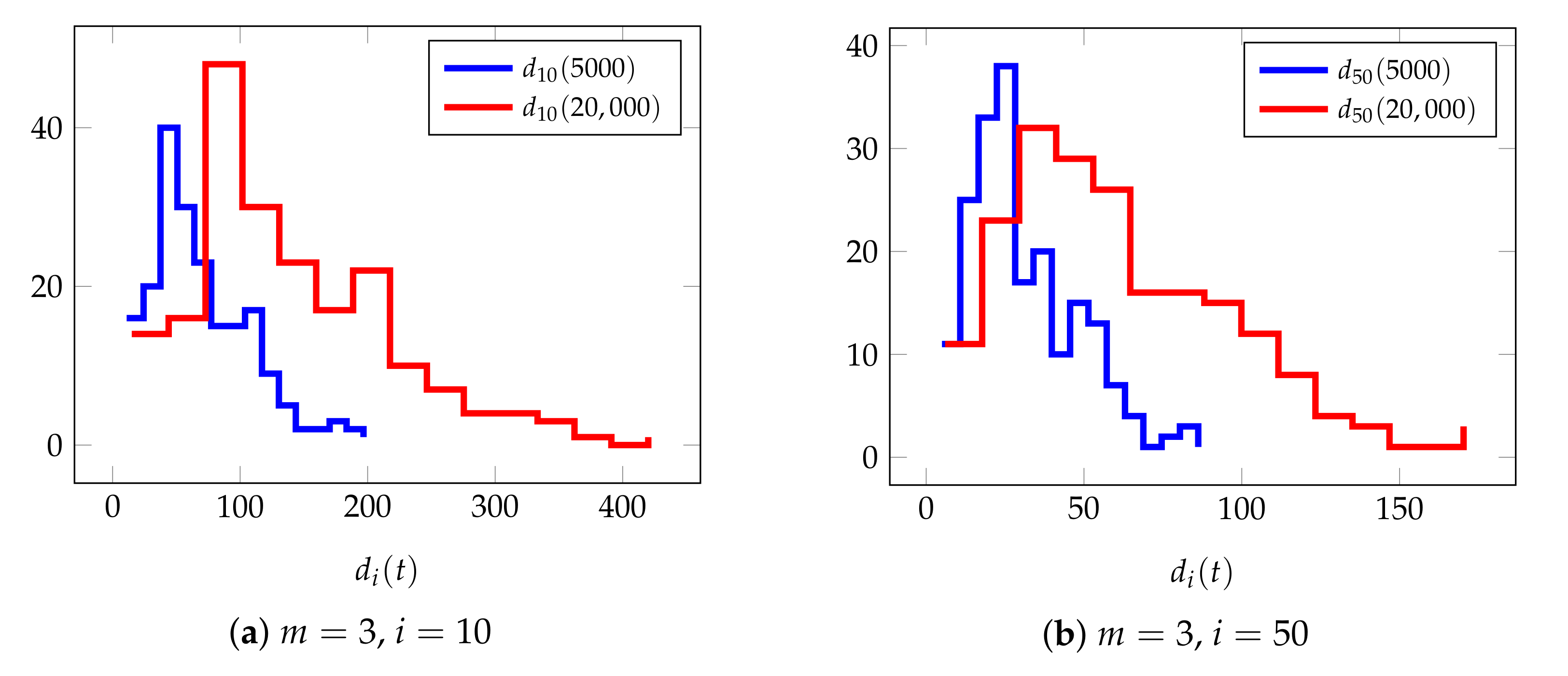
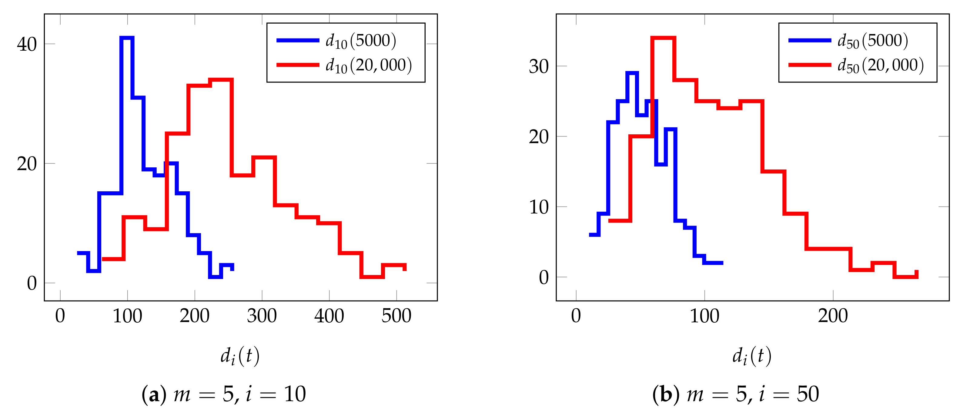
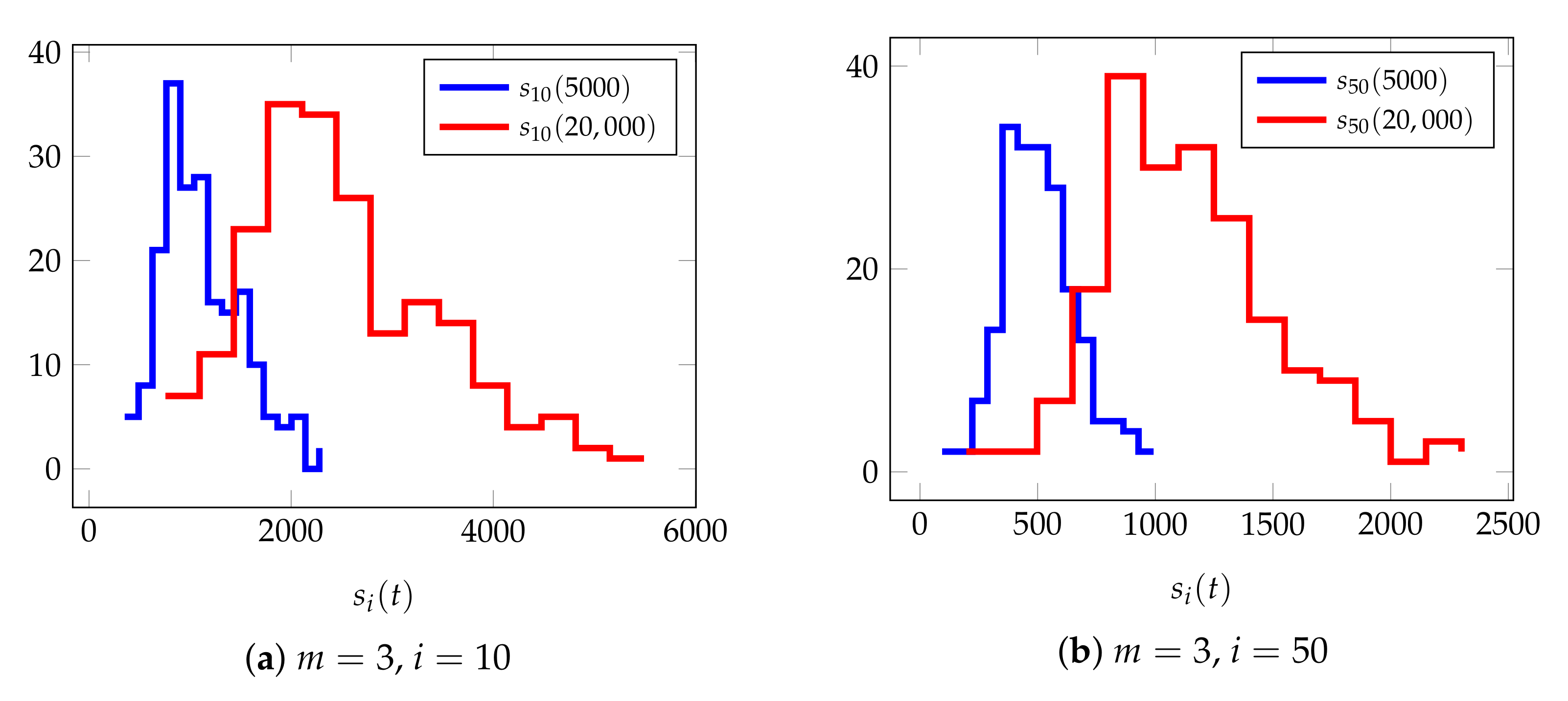
The stationarity of stochastic processes means that the distribution parameters of a random variable remain unchanged over time. Obviously, the processes under consideration are not stationary. This can clearly be seen in Figure 1, Figure 2, Figure 3 and Figure 4, which show empirical histograms of distributions of random variables $d_i\left(t\right)$ and $s_i\left(t\right)$ based on different realizations of their trajectories. The histograms were obtained as follows: we simulated the evolution of the BA graphs 200 times and obtained 200 corresponding values of random variables $d_i\left(t\right)$ and $s_i\left(t\right)$ for two nodes $i=10$ and $i=50$ at iterations $t=5000$ and $t=$ 20,000. To construct the histograms, we used the number of bins equal to 15. Figure 1 and Figure 2 represent histograms of $d_i$ and were obtained for $m=3$ and $m=5$, respectively. Figure 3 and Figure 4 show histograms of $s_i$ and were obtained for $m=3$ and $m=5$, respectively. The empirical values of the characteristics of the distributions of random variables are presented in Table 1, Table 2, Table 3 and Table 4.

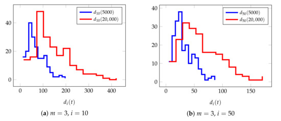
Figure 1. The histograms of the empirical values of $d_i\left(t\right)$ obtained by stimulating 200 different networks with $m=3$ at iterations 5000 (blue line) and 20,000 (red line), (a) for node $i=10$, (b) for node $i=50$.

Figure 2. The histograms of the empirical values of $d_i\left(t\right)$ obtained by stimulating 200 different networks with $m=5$ at iterations 5000 (blue line) and 20,000 (red line), (a) for node $i=10$, (b) for node $i=50$.

Figure 3. The histograms of the empirical values of $s_i\left(t\right)$ obtained by stimulating 200 different networks with $m=3$ at iterations 5000 (blue line) and 20,000 (red line), (a) for node $i=10$, (b) for node $i=50$.

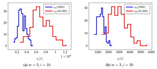
Figure 4. The histograms of the empirical values of $s_i\left(t\right)$ obtained by stimulating 200 different networks with $m=5$ at iterations 5000 (blue line) and 20,000 (red line), (a) for node $i=10$, (b) for node $i=50$.

Table 1. Empirical characteristics of the $d_i$-distribution obtained by simulating 200 different Barabási–Albert networks with $m=3$, for nodes $i=10$ and $i=50$ at iterations 5000 and 20,000.

	${\mathit{d}}_{10}\left(5000\right)$	${\mathit{d}}_{10}$(20,000)	${\mathit{d}}_{50}\left(5000\right)$	${\mathit{d}}_{50}$(20,000)
mean	70.85	141.09	31.92	62.65
st.dev.	38.88	79.06	17.68	35.89
skewness	0.97	1.01	0.92	0.91
kurtosis	3.76	4.01	3.58	3.58

Table 2. Empirical characteristics of the $d_i$-distribution obtained by simulating 200 different Barabási–Albert networks with $m=5$, for nodes $i=10$ and $i=50$ at iterations 5000 and 20,000.

	${\mathit{d}}_{10}\left(5000\right)$	${\mathit{d}}_{10}$(20,000)	${\mathit{d}}_{50}\left(5000\right)$	${\mathit{d}}_{50}$(20,000)
mean	127.41	253.52	52.54	105.37
st.dev.	46.68	93.51	21.60	44.66
skewness	0.52	0.52	0.58	0.78
kurtosis	3.24	3.11	3.19	3.80

Table 3. Empirical characteristics of the $s_i$-distribution obtained by simulating 200 different Barabási–Albert networks with $m=3$, for nodes $i=10$ and $i=50$ at iterations 5000 and 20,000.

	${\mathit{s}}_{10}\left(5000\right)$	${\mathit{s}}_{10}$(20,000)	${\mathit{s}}_{50}\left(5000\right)$	${\mathit{s}}_{50}$(20,000)
mean	1120.17	2534.05	513.34	1155.37
st.dev.	398.22	957.09	165.09	387.56
skewness	0.74	0.80	0.61	0.68
kurtosis	3.25	3.44	3.69	3.74

Table 4. Empirical characteristics of the $d_i$-distribution obtained by simulating 200 different Barabási–Albert networks with $m=5$, for nodes $i=10$ and $i=50$ at iterations 5000 and 20,000.

	${\mathit{s}}_{10}\left(5000\right)$	${\mathit{s}}_{10}$(20,000)	${\mathit{s}}_{50}\left(5000\right)$	${\mathit{s}}_{50}$(20,000)
mean	3037.39	6947.17	1277.91	2915.58
st.dev.	773.23	1867.67	318.93	774.61
skewness	0.28	0.32	0.41	0.51
kurtosis	3.14	3.09	3.32	3.23

Experimental results show that both distributions have mean values that increase over time. In addition, the growth of their standard deviations is proportional to the increase in their means. The values of the skewness coefficient are positive in all cases, which indicate the asymmetry of the distributions. Kurtosis is greater than 3, which means that their tails are thicker than the tail of normal distribution.

2.3. The Evolution of the Barabási–Albert Networks

It follows from the definition of the Barabási–Albert network that

• If ${\xi }^{t+1}=i$, then $d_i(t+1)=d_i\left(t\right)+1$ and $s_i(t+1)=s_i\left(t\right)+m$, as the result of joining node $v_i$ with newborn node $v_{t+1}$ of degree m.
• If ${\xi }^{t+1}=j$ and $(v_j,v_i)\in V_t$, i.e., new node $v_{t+1}$ joins a neighbor $v_j$ of node $v_i$, then $d_i(t+1)=d_i\left(t\right)$ and $s_i(t+1)=s_i\left(t\right)+1$.

Let ${\xi }_i^{t+1}=1$ if node $v_{t+1}$ links to node $v_i$ at iteration $t+1$, and ${\xi }_i^{t+1}=0$ otherwise; i.e.,

$${\xi }_i^{t+1}=\left\{\begin{array}{c}1,(v_{t+1},v_i)\in V_{t+1}\hfill \\ 0,\mathrm{otherwise}.\hfill \end{array}\right.$$

Let ${\eta }_i^{t+1}=1$ if node $v_{t+1}$ links to one of the neighbors of node $v_i$ at iteration $t+1$, and ${\eta }_i^{t+1}=0$ otherwise; i.e.,

$${\eta }_i^{t+1}=\left\{\begin{array}{c}1,(v_{t+1},v_j)\in V_{t+1}\mathrm{and}(v_j,v_i)\in V_t,\hfill \\ 0,\mathrm{otherwise}.\hfill \end{array}\right.$$

Then the conditional expectations of ${\xi }_i^{t+1}$ and ${\eta }_i^{t+1}$ at moment $t+1$ are equal to

$$\mathbb{E}\left({\xi }_i^{t+1}\right|G_t)=\frac{d_i\left(t\right)}{2t},\mathbb{E}\left({\eta }_i^{t+1}\right|G_t)=\frac{s_i\left(t\right)}{2t},$$

(3)

Let ${\mu }_n\left(\xi \right)$ denote n-th central moment of a random variable $\xi$ defined by

$${\mu }_n\left(\xi \right)=\mathbb{E}{(\xi -\mathbb{E}\left(\xi \right))}^n,n\in \mathbb{N}.$$

(4)

Due to the linearity of the mathematical expectation, the following formula holds for finding the n-th central moment of a random variable:

$${\mu }_n\left(\xi \right)=\sum _{i=0}^n{(-1)}^i\left(\genfrac{}{}{0pt}{}{n}{i}\right){\nu }_{n-i}\left(\xi \right){\nu }_1^i\left(\xi \right),$$

where ${\nu }_i\left(\xi \right)$ is i-th moment defined by

$${\nu }_i\left(\xi \right)=\mathbb{E}\left({\xi }^i\right).$$

Indeed, it follows from Equation (4) that we have

$$\begin{array}{c}{\mu }_n=\mathbb{E}\left(\sum _{i=0}^n{(-1)}^i\left(\genfrac{}{}{0pt}{}{n}{i}\right){\mathbb{E}}^i\left(\xi \right){\xi }^{n-i}\right)=\hfill \\ \hfill \sum _{i=0}^n{(-1)}^i\left(\genfrac{}{}{0pt}{}{n}{i}\right){\mathbb{E}}^i\left(\xi \right)\mathbb{E}\left({\xi }^{n-i}\right)=\sum _{i=0}^n{(-1)}^i\left(\genfrac{}{}{0pt}{}{n}{i}\right){\nu }_1^i{\nu }_{n-i}.\end{array}$$

(5)

The variance is the second central moment of the random variable, i.e., ${\mu }_2\left(\xi \right)=\mathrm{Var}\left(\xi \right)$.

3. Node Degree Dynamics: The Evolution of Its Variation and High-Order Moments in Time

3.1. The Variation of $d_i\left(t\right)$

Lemma 1.

The second moment of $d_i\left(t\right)$ follows

$$\mathbb{E}\left(d_i^2\left(t\right)\right)=m(m+1)\frac{t}{i}-m{\left(\frac{t}{i}\right)}^{\frac{1}{2}}.$$

(6)

Proof. 

We have

$$\begin{array}{c}\Delta d_i^2(t+1):=d_i^2(t+1)-d_i^2\left(t\right)=\hfill \\ \hfill {(d_i\left(t\right)+1)}^2{\xi }_i^{t+1}+d_i^2\left(t\right)(1-{\xi }_i^{t+1})-d_i^2\left(t\right)=(2d_i\left(t\right)+1){\xi }_i^{t+1}.\end{array}$$

(7)

It follows from (3) that the conditional expectation of $d_i^2(t+1)$ at iteration $t+1$ is

$$\mathbb{E}\left(d_i^2\left(t\right)\right|G_t)=(2d_i\left(t\right)+1)\frac{d_i\left(t\right)}{2t}=\frac{d_i^2\left(t\right)}{t}+\frac{d_i\left(t\right)}{2t}.$$

(8)

Now let us pass from the difference equation, Equation (8), to its approximate version of the differential equation, denoting $\mathrm{E}\left(d_i^2\left(t\right)\right)$ as $f\left(t\right)$, replacing $\Delta f\left(t\right)$ with $\frac{df\left(t\right)}{dt}$, and replacing $d_i\left(t\right)$ with its expectation $m{\left(\frac{t}{i}\right)}^{\frac{1}{2}}$. Then, we get

$$\frac{df\left(t\right)}{dt}=\frac{f\left(t\right)}{t}+\frac{m}{2{\left(ti\right)}^{\frac{1}{2}}},$$

the solution of which is $f\left(t\right)=ct-m{\left(\frac{t}{i}\right)}^{\frac{1}{2}}$. Since $d_i\left(i\right)=m$, i.e., $d_i^2\left(i\right)=m^2$, we get $c=m(m+1)$. Thus, we get (6). □

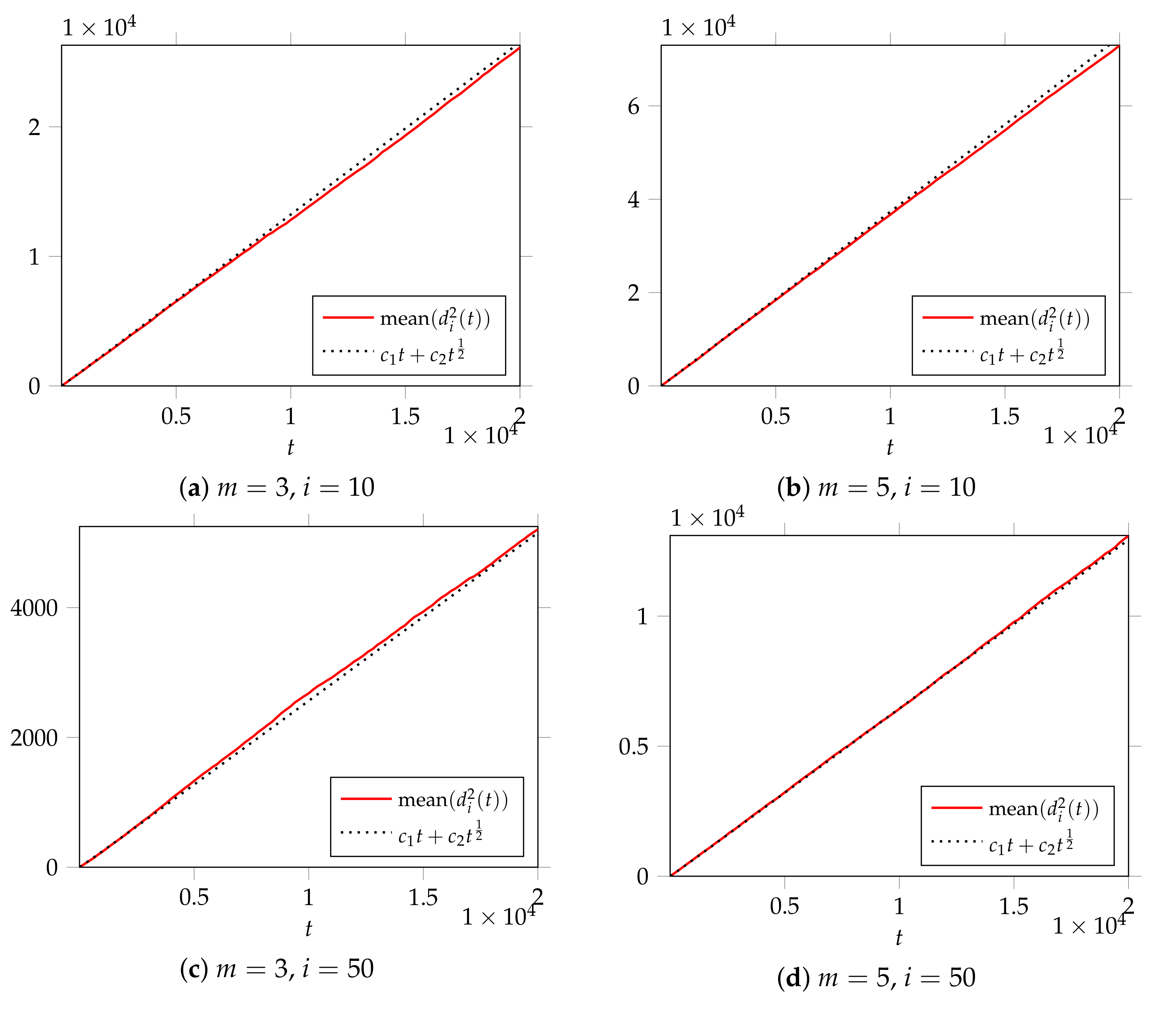
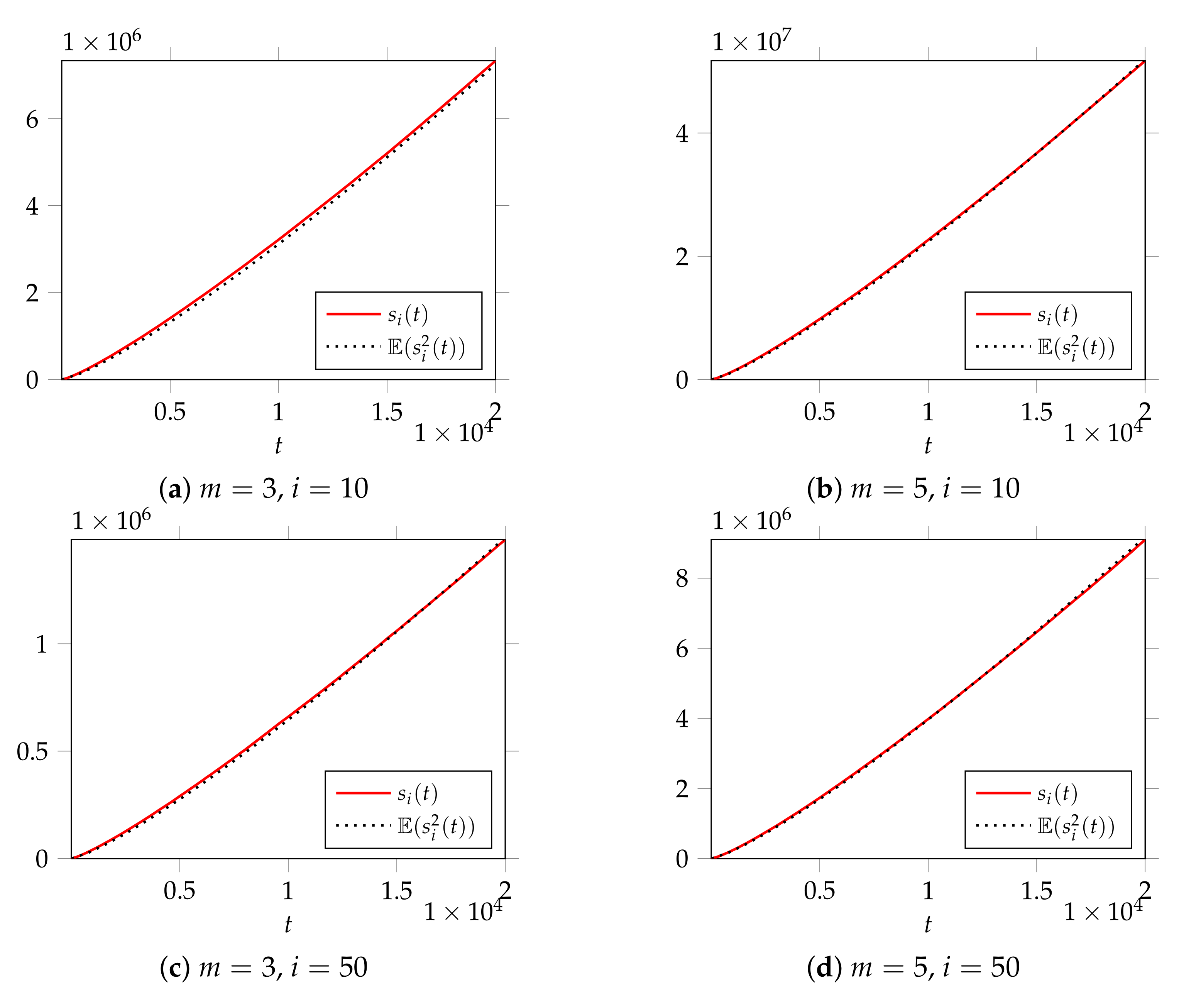
To illustrate the result, we carried out $T=200$ independent repetitions in which BA graph evolution was simulated 200 times, each time for $N=$ 20,000 iterations, for different values $m=3$ and $m=5$. Then we obtained the mean of the empirical values of $d_i^2\left(t\right)$. The results are presented in Figure 5.

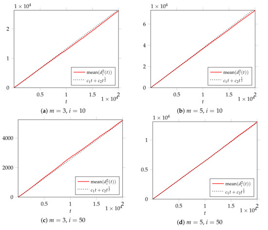
Figure 5. Dynamics of empirical values for $\mathrm{Mean}\left(d_i^2\left(t\right)\right)$ in networks based on BA model for selected nodes $i=10,50$ as t iterates up to 20,000. Network in (a) is modeled with $m=3$, $i=10$, (b) with $m=5$, $i=10$, (c) with $m=3$, $i=50$, (d) with $m=5$, $i=50$.

Theorem 1.

The variation of $d_i\left(t\right)$ at iteration t is

$$\mathrm{Var}\left(d_i\left(t\right)\right)=m\left(\frac{t}{i}-{\left(\frac{t}{i}\right)}^{\frac{1}{2}}\right).$$

Proof. 

The definition of variation implies

$$\mathrm{Var}\left(d_i\left(t\right)\right)=\mathbb{E}\left(d_i^2\left(t\right)\right)-{\mathbb{E}}^2\left(d_i\left(t\right)\right).$$

(9)

Then Theorem follows from Lemma 1 and the estimate $\mathbb{E}\left(d_i\left(t\right)\right)=m{\left(\frac{t}{i}\right)}^{\frac{1}{2}}$ (see Equation (2)). □

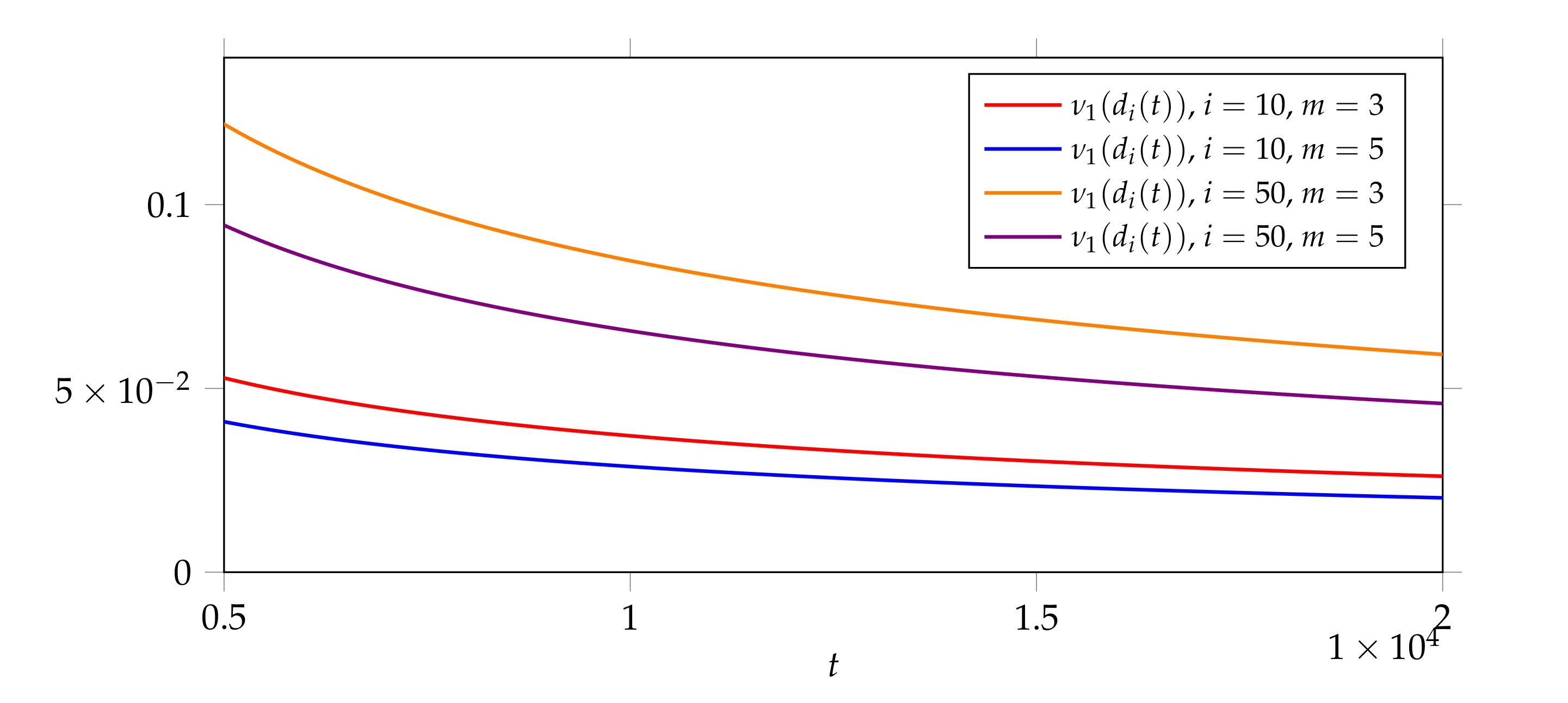
The standard deviation of $d_i\left(t\right)$, defined as $\sqrt{\mathrm{Var}\left(d_i\left(t\right)\right)}$, is the same order of magnitude as $\mathbb{E}\left(d_i\left(t\right)\right)$:

$$\frac{\mathbb{E}\left(d_i\left(t\right)\right)}{\sqrt{\mathrm{Var}\left(d_i\left(t\right)\right)}}\to \sqrt{\frac{m+1}{m}}\mathrm{as}t\to \infty ,$$

i.e., the coefficient of variation for $d_i\left(t\right)$ tends to $\frac{m+1}{m}>1$ as t tends to ∞. Thus, the $d_i\left(t\right)$-distribution is high-variance.

3.2. The High-Order Moments of $d_i\left(t\right)$

Theorem 2.

$$\mathbb{E}\left(d_i^n\left(t\right)\right)\sim C(n,m){\left(\frac{t}{i}\right)}^{\frac{n}{2}}+O\left(t^{\frac{n-1}{2}}\right),$$

where $C(n,m)=m(m+1)\dots (m+n-1)$ depends on n and m only.

Proof. 

We have

$$\Delta d_i^n(t+1):=d_i^n(t+1)-d_i^n\left(t\right)={(d_i\left(t\right)+1)}^n{\xi }_i^{t+1}+d_i^n\left(t\right)\left(1-{\xi }_i^{t+1}\right)-d_i^n\left(t\right).$$

Then it follows from (3) that

$$\begin{array}{c}\mathbb{E}(\Delta d_i^n(t+1)|G_t)=\frac{d_i\left(t\right)}{2t}({(d_i\left(t\right)+1)}^n-d_i^n\left(t\right))=\frac{d_i\left(t\right)}{2t}\sum _{j=0}^{n-1}\left(\genfrac{}{}{0pt}{}{n}{j}\right)d_i^j\left(t\right)=\hfill \\ \hfill \frac{1}{2t}\sum _{j=0}^{n-1}\left(\genfrac{}{}{0pt}{}{n}{j}\right)d_i^{j+1}\left(t\right)=\frac{1}{2t}\left(n{d}_i^n\left(t\right)+\sum _{j=0}^{n-2}\left(\genfrac{}{}{0pt}{}{n}{j}\right)d_i^{j+1}\left(t\right)\right).\end{array}$$

Assuming that $\mathbb{E}\left(d_i^m\left(t\right)\right)$ are obtained for all $m\in \{1,\dots ,n-1\}$, the expectation of ${\sum }_{j=0}^{n-2}\left(\genfrac{}{}{0pt}{}{n}{j}\right)d_i^{j+1}$ can be found with the use of linearity of expectation. Taking the expectation of both sides and denoting $d_i^n\left(t\right)$ and ${\sum }_{j=0}^{n-2}\left(\genfrac{}{}{0pt}{}{n}{j}\right)\mathbb{E}\left(d_i^{j+1}\right)$ by $f\left(t\right)$ and $g\left(t\right)$, respectively, we get the following differential equation

$$\frac{df}{dt}=\frac{nf}{2t}+\frac{g}{2t}.$$

We get its solution in the following form:

$$f\left(t\right)=\frac{t^{\frac{n}{2}}}{2}\int t^{-\frac{n}{2}-1}g\left(t\right)dt+C{t}^{\frac{n}{2}},$$

and we obtain the recurrent formula for finding $\mathbb{E}\left(d_i^n\left(t\right)\right)$:

$$\mathbb{E}\left(d_i^n\left(t\right)\right))=\frac{t^{\frac{n}{2}}}{2}\int t^{-\frac{n}{2}-1}\sum _{j=0}^{n-2}\left(\genfrac{}{}{0pt}{}{n}{j}\right)\mathbb{E}\left(d_i^{j+1}\left(t\right)\right)dt+C{t}^{\frac{n}{2}},$$

(10)

where constant C can be found from the initial condition $\mathbb{E}\left(d_i^n\left(i\right)\right))=m^n$.

Let us show by induction that

$$\mathbb{E}\left(d_i^n\left(t\right)\right)=C_1{\left(\frac{t}{i}\right)}^{\frac{1}{2}}+C_2{\left(\frac{t}{i}\right)}^{\frac{2}{2}}+s+C_n{\left(\frac{t}{i}\right)}^{\frac{n}{2}}.$$

(11)

Indeed, if $n=1$, we get the well-known estimate $\mathbb{E}\left(d_i\left(t\right)\right)=m{\left(\frac{t}{i}\right)}^{\frac{1}{2}}$.

Suppose that (11) is true for all $n^{\prime }<n$. We will show that (11) is also fulfilled for $n^{\prime }=n$. We have

$$\mathbb{E}\left(d_i^n\left(t\right)\right))=\frac{t^{\frac{n}{2}}}{2}\int t^{-\frac{n}{2}-1}\sum _{j=0}^{n-2}\left(\genfrac{}{}{0pt}{}{n}{j}\right)\mathbb{E}\left(d_i^{j+1}\left(t\right)\right)dt+C{t}^{\frac{n}{2}},$$

by the induction hypothesis. The sum ${\sum }_{j=0}^{n-2}\left(\genfrac{}{}{0pt}{}{n}{j}\right)\mathbb{E}\left(d_i^{j+1}\right)$ can be presented as

$$C_1{\left(\frac{t}{i}\right)}^{\frac{1}{2}}+C_2{\left(\frac{t}{i}\right)}^{\frac{2}{2}}+\dots +C_{n-1}{\left(\frac{t}{i}\right)}^{\frac{n-1}{2}}.$$

Then the whole integral will be the sum of integrals of the form $\int t^{-\frac{n}{2}-1}{C}_p{\left(\frac{t}{i}\right)}^{\frac{p}{2}}dt$, where $p\in \{1,\dots ,n-1\}$, each of which is equal to $C_p^{\prime }{t}^{\frac{p-n}{2}}{i}^{-\frac{p}{2}}$. Therefore, we get

$$\begin{array}{c}\mathbb{E}\left(d_i^n\left(t\right)\right)=\frac{t^{\frac{n}{2}}}{2}\sum _{p=1}^{n-1}{C}_p^{\prime }{t}^{\frac{p-n}{2}}{i}^{-\frac{p}{2}}+C{t}^{\frac{n}{2}}=\sum _{p=1}^{n-1}{C}_p^{\prime }{\left(\frac{t}{i}\right)}^{\frac{p}{2}}+C{t}^{\frac{n}{2}}=\hfill \\ \hfill C_1^{\prime }{\left(\frac{t}{i}\right)}^{\frac{1}{2}}+C_2^{\prime }{\left(\frac{t}{i}\right)}^{\frac{2}{2}}+\cdots +C_n{\left(\frac{t}{i}\right)}^{\frac{n}{2}}.\end{array}$$

□

3.3. The Skewness of $d_i\left(t\right)$

The asymmetry coefficient ${\gamma }_1\left(\xi \right)$ of a random variable $\xi$ is defined by

$${\gamma }_1\left(\xi \right)=\frac{{\mu }_3\left(\xi \right)}{{\mu }_2^{3/2}\left(\xi \right)},$$

where ${\mu }_3\left(\xi \right)$ and ${\mu }_2\left(\xi \right)$ are the third and the second central moments of the $\xi$-distribution, respectively.

Lemma 2.

The third moment of $d_i\left(t\right)$ follows

$$\mathbb{E}\left(d_i^3\left(t\right)\right))=m(m+1)(m+2){\left(\frac{t}{i}\right)}^{\frac{3}{2}}-3m(m+1)\frac{t}{i}+m{\left(\frac{t}{i}\right)}^{\frac{1}{2}}.$$

(12)

Proof. 

Using Equation (10), we can find $\mathbb{E}\left(d_i^3\left(t\right)\right)$:

$$\begin{array}{c}\mathbb{E}\left(d_i^3\left(t\right)\right))=\frac{t^{\frac{3}{2}}}{2}\int t^{-\frac{5}{2}}\sum _{j=0}^1\left(\genfrac{}{}{0pt}{}{3}{j}\right)\mathbb{E}\left(d_i^{j+1}\right)dt+C{t}^{\frac{3}{2}}=\hfill \\ \frac{t^{\frac{3}{2}}}{2}\int t^{-\frac{5}{2}}\left(\mathbb{E}\left(d_i\right)+3\mathbb{E}\left(d_i^2\right)\right)dt+C{t}^{\frac{3}{2}}=\\ \frac{t^{\frac{3}{2}}}{2}\int t^{-\frac{5}{2}}\left(m\sqrt{\frac{t}{i}}+3\left(m(m+1)\frac{t}{i}-m\sqrt{\frac{t}{i}}\right)\right)dt+C{t}^{\frac{3}{2}}=\\ \hfill m\sqrt{\frac{t}{i}}-3m(m+1)\frac{t}{i}+C{t}^{\frac{3}{2}}.\end{array}$$

We have

$$\mathbb{E}\left(d_i^3\left(i\right)\right))=m^3\Rightarrow C=\frac{m^3+3m^2+2m}{i^{\frac{3}{2}}}=\frac{m(m+1)(m+2)}{i^{\frac{3}{2}}}.$$

Therefore, we get (12). □

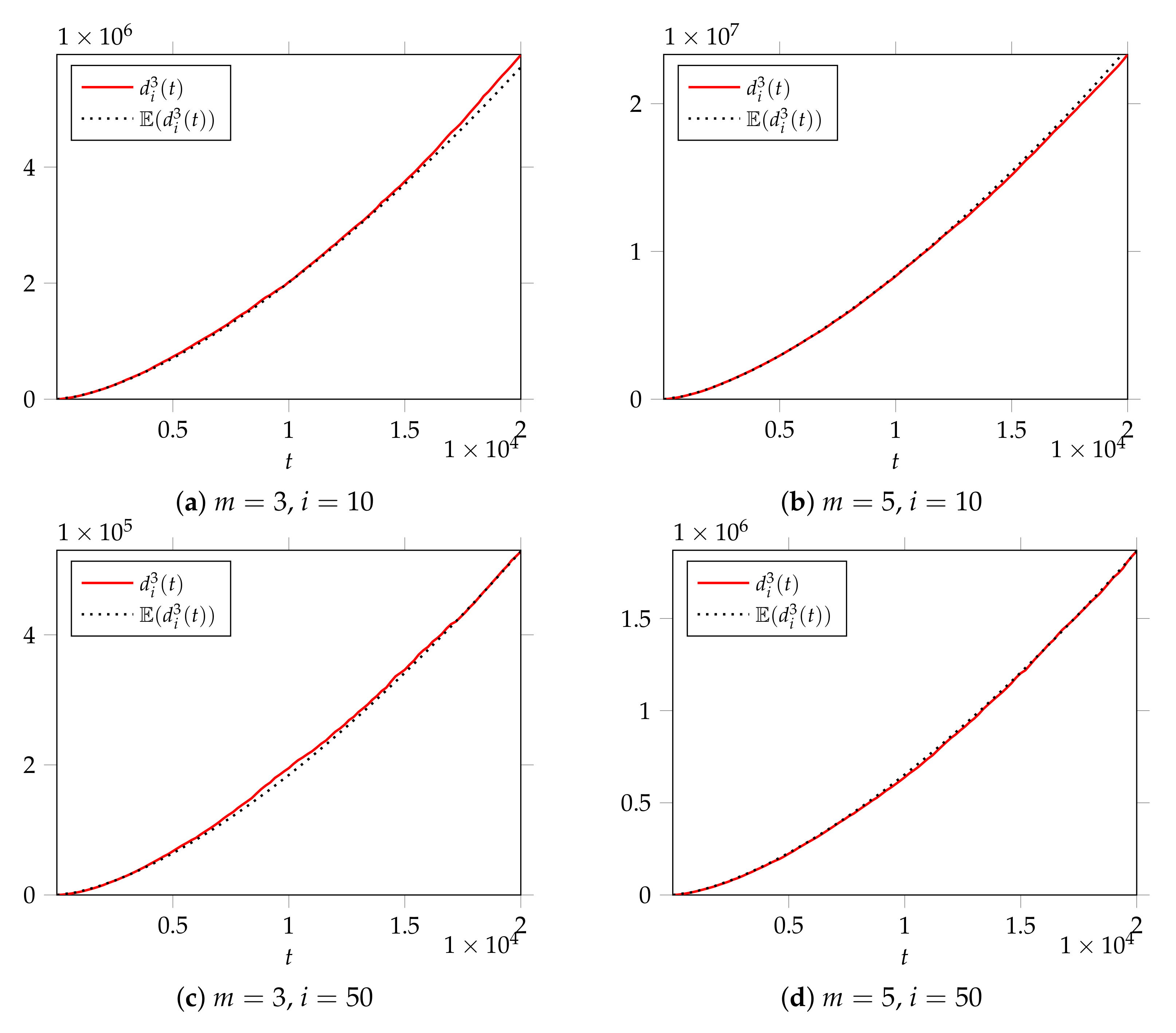
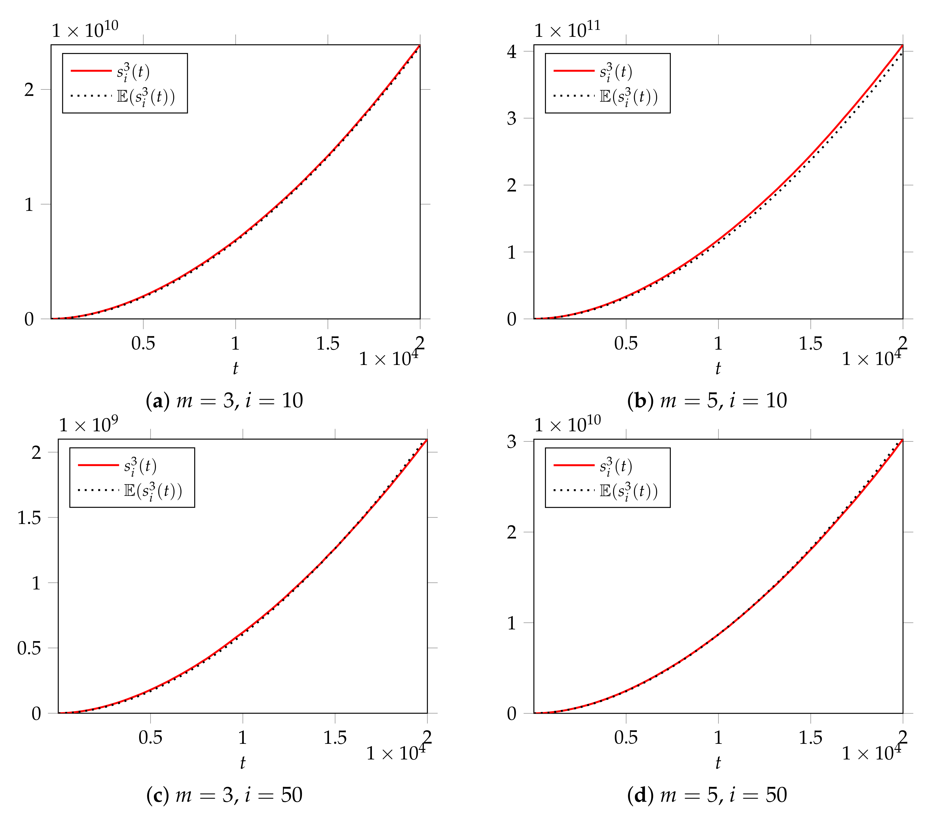
To exhibit the result, we carried out $T=200$ independent repetitions; in each of them, the BA graph was simulated for $N=$ 20,000 iterations, for different values $m=3$ and $m=5$. Then the empirical values of $\mathrm{mean}\left(d_i^3\left(t\right)\right)$ were obtained. The results are presented in Figure 6.

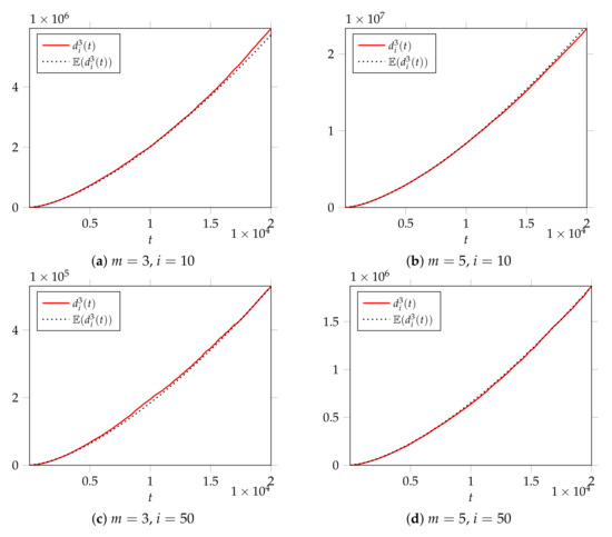
Figure 6. Dynamics of empirical values for $\mathrm{Mean}\left(d_i^3\left(t\right)\right)$ in networks based on BA model for selected nodes $i=10,50$ as t iterates up to 20,000. Network in (a) is modeled with $m=3$, $i=10$, (b) with $m=5$, $i=10$, (c) with $m=3$, $i=50$, (d) with $m=5$, $i=50$.

Theorem 3.

The asymmetry coefficient ${\gamma }_1\left(d_i\left(t\right)\right)$ for the distribution of $d_i\left(t\right)$ follows

$${\gamma }_1\left(d_i\left(t\right)\right)\sim \frac{2{\left(\frac{t}{i}\right)}^{\frac{1}{2}}-1}{m^{\frac{1}{2}}{\left(\frac{t}{i}\right)}^{\frac{1}{4}}{\left({\left(\frac{t}{i}\right)}^{\frac{1}{2}}-1\right)}^{\frac{1}{2}}}.$$

Proof. 

Using Equation (5) we can find the third central moments ${\mu }_3\left(d_i\right)$ as follows

$${\mu }_3\left(d_i\left(t\right)\right)=\mathbb{E}\left(d_i^3\right)-3\mathbb{E}\left(d_i^2\right)\mathbb{E}\left(d_i\right)+2{\mathbb{E}}^3\left(d_i\right)=m{\left(\frac{t}{i}\right)}^{\frac{1}{2}}-3m\left(\frac{t}{i}\right)+2m{\left(\frac{t}{i}\right)}^{\frac{3}{2}}.$$

Therefore, using Theorem 1 we have

$$\begin{array}{cc}{\gamma }_1\left(d_i\left(t\right)\right):=\frac{{\mu }_3\left(d_i\left(t\right)\right)}{{\mu }_2^{3/2}\left(d_i\left(t\right)\right)}=\hfill & \frac{m{\left(\frac{t}{i}\right)}^{\frac{1}{2}}-3m\left(\frac{t}{i}\right)+2m{\left(\frac{t}{i}\right)}^{\frac{3}{2}}}{{\left(m\left(\frac{t}{i}-\sqrt{\frac{t}{i}}\right)\right)}^{\frac{3}{2}}}=\hfill \\ & \frac{m{\left(\frac{t}{i}\right)}^{\frac{1}{2}}\left({\left(\frac{t}{i}\right)}^{\frac{1}{2}}-1\right)\left(2{\left(\frac{t}{i}\right)}^{\frac{1}{2}}-1\right)}{m^{\frac{3}{2}}{\left(\frac{t}{i}\right)}^{\frac{3}{4}}{\left({\left(\frac{t}{i}\right)}^{\frac{1}{2}}-1\right)}^{\frac{3}{2}}}=\frac{2{\left(\frac{t}{i}\right)}^{\frac{1}{2}}-1}{m^{\frac{1}{2}}{\left(\frac{t}{i}\right)}^{\frac{1}{4}}{\left({\left(\frac{t}{i}\right)}^{\frac{1}{2}}-1\right)}^{\frac{1}{2}}}.\hfill \end{array}$$

□

Remark 2.

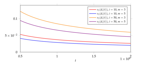
It follows from Theorem 3 that ${\gamma }_1\left(d_i\left(t\right)\right)>0$ for all $t\ge i$, therefore, the distribution of $d_i\left(t\right)$ is asymmetric, and its right tail is thicker than the left tail. The initial value of the asymmetry coefficient is 4 $m^{-1/2}$. However, ${\gamma }_1\left(d_i\left(t\right)\right)\to$ 2 $m^{-1/2}$ as $t\to \infty$. Therefore, its value decreases with the network growth (see Figure 7).

Figure 7. Evolution of asymmetry coefficient in BA networks for selected nodes $i=10$ and $i=50$ as t iterates up to 20,000.

3.4. The Kurtosis of $d_i\left(t\right)$

Using Equation (10), we can find $\mathbb{E}\left(d_i^4\left(t\right)\right)$:

$$\begin{array}{c}\mathbb{E}\left(d_i^4\left(t\right)\right)=m(m+1)(m+2)(m+3){\left(\frac{t}{i}\right)}^2-\hfill \\ \hfill 6m(m+1)(m+2){\left(\frac{t}{i}\right)}^{\frac{3}{2}}+7m(m+1)\frac{t}{i}-m{\left(\frac{t}{i}\right)}^{\frac{1}{2}},\end{array}$$

(13)

which in turn can be used to find the kurtosis of $d_i$.

Theorem 4.

The kurtosis of $d_i$ follows

$$\mathrm{Kurt}\left(d_i\left(t\right)\right)\sim \frac{\left(\frac{t}{i}-{\left(\frac{t}{i}\right)}^{\frac{1}{2}}\right)\left(3m(m+2)\left(\frac{t}{i}-{\left(\frac{t}{i}\right)}^{\frac{1}{2}}\right)+m\right)}{m^2{\left(\frac{t}{i}-{\left(\frac{t}{i}\right)}^{\frac{1}{2}}\right)}^2}.$$

(14)

Proof. 

By definition of kurtosis, we have

$$\mathrm{Kurt}\left(d_i\left(t\right)\right):=\frac{{\mu }_4\left(d_i\left(t\right)\right)}{{\mathrm{Var}}^2\left(d_i\left(t\right)\right)},$$

where

$$\begin{array}{c}{\mu }_4\left(d_i\left(t\right)\right)=\mathbb{E}{(d_i\left(t\right)-\mathbb{E}\left(d_i\left(t\right)\right))}^4=\hfill \\ \mathbb{E}\left(d_i^4\left(t\right)\right)-4\mathbb{E}\left(d_i\left(t\right)\right)\mathbb{E}\left(d_i^3\left(t\right)\right)+6{\mathbb{E}}^2\left(d_i\left(t\right)\right)\mathbb{E}\left(d_i^2\left(t\right)\right)-3{\mathbb{E}}^4\left(d_i\left(t\right)\right)=\\ \hfill \left(\frac{t}{i}-{\left(\frac{t}{i}\right)}^{\frac{1}{2}}\right)\left(3m(m+2)\left(\frac{t}{i}-{\left(\frac{t}{i}\right)}^{\frac{1}{2}}\right)+m\right).\end{array}$$

(15)

Thus, we get (14). □

Remark 3.

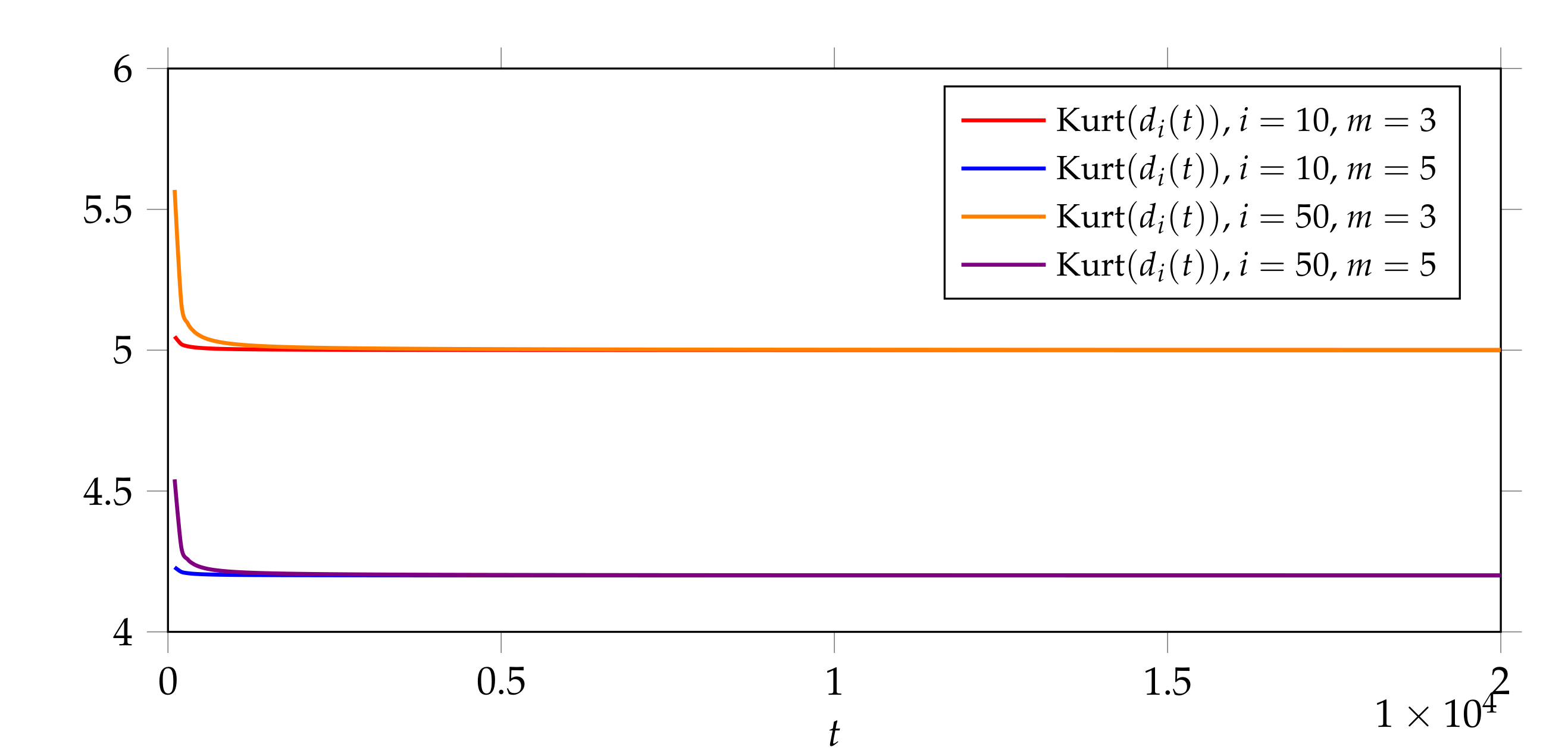
Equation (14) implies $\mathrm{Kurt}\left(d_i\left(t\right)\right)>\frac{3(m+2)}{m}$ for all t. Moreover, $\mathrm{Kurt}\left(d_i\left(t\right)\right)$ gradually decreases to $\frac{3(m+2)}{m}$ as t tends to infinity (see Figure 8). This means that the distribution of $d_i\left(t\right)$ is heavy-tailed for small t and is close to normal distribution for large t and large m.

Figure 8. Evolution of kurtosis in BA networks for selected nodes $i=10$ and $i=50$ as t iterates up to 20,000.

-0.6cm0cm

4. The Dynamics of ${\mathit{s}}_{\mathit{i}}\left(\mathit{t}\right)$: Its Variation, Asymmetry Coefficient and Kurtosis

In this section, we consider the random variable $s_i\left(t\right)$, which is defined as the sum of the degrees of the $v_i$-vertex neighbors at the time t. The mathematical expression of this random variable $\mathbb{E}\left(s_i\left(t\right)\right)$ is found in the works [27] (for $m=1$) and [28] (for arbitrary m):

$$\mathbb{E}\left(s_i\left(t\right)\right)=\frac{m^2}{2}{\left(\frac{t}{i}\right)}^{\frac{1}{2}}(logt+C),$$

(16)

where C is a constant.

In this section, the dynamics of the stochastic process of $s_i\left(t\right)$ is investigated a little deeper, namely, the dynamics of the second, third and fourth moments are found, i.e., $\mathbb{E}\left(s_i^n\left(t\right)\right)$, $n=2,3,4$, which allow us to estimate the variation, the asymmetry coefficient and the kurtosis of $s_i\left(t\right)$.

4.1. The Second Moment and the Variation of $s_i\left(t\right)$

We first find the exact value of constant C from Equation (16).

Let $P(i,j)$ denote the probability that vertex $v_i$ is connected to the vertex $v_j$ at the moment of its appearance at time i, i.e., $P(i,j)=\frac{d_j\left(i\right)}{2i}$. We get

$$\mathbb{E}\left(s_i\left(i\right)\right)=\mathbb{E}\left(\sum _{j=1}^{i-1}P(i,j)d_j\left(i\right)\right)=\mathbb{E}\left(\sum _{j=1}^{i-1}\frac{d_j^2\left(i\right)}{2i}\right)=\frac{1}{2i}\sum _{j=1}^{i-1}\mathbb{E}\left(d_j^2\left(i\right)\right).$$

Since

$$\mathbb{E}\left(d_i^2\left(t\right)\right)=m(m+1)\frac{t}{i}-m{\left(\frac{t}{i}\right)}^{\frac{1}{2}},$$

we can continue equality as follows:

$$\begin{array}{c}\mathbb{E}\left(s_i\left(i\right)\right)=\frac{1}{2i}\sum _{j=1}^{i-1}\left(m(m+1)\frac{i}{j}-m{\left(\frac{i}{j}\right)}^{\frac{1}{2}}\right)=\hfill \\ \frac{1}{2i}\left(m(m+1)i\sum _{j=1}^{i-1}\frac{1}{j}-m\sqrt{i}\sum _{j=1}^{i-1}\frac{1}{\sqrt{j}}\right)\approx \\ \hfill \frac{1}{2i}\left(m(m+1)ilogi-m\sqrt{i}2\sqrt{i}\right)=\frac{m}{2}((m+1)logi-2).\end{array}$$

(17)

Therefore,

$$\mathbb{E}\left(s_i\left(i\right)\right)=\frac{m^2}{2}(logi+C)=\frac{m}{2}((m+1)logi-2)\Rightarrow C=\frac{1}{m}(logi-2),$$

(18)

and we finally get

$$\mathbb{E}\left(s_i\left(t\right)\right)=\frac{m^2}{2}{\left(\frac{t}{i}\right)}^{\frac{1}{2}}\left(logt+\frac{1}{m}logi-\frac{2}{m}\right).$$

(19)

This result will be useful to us later.

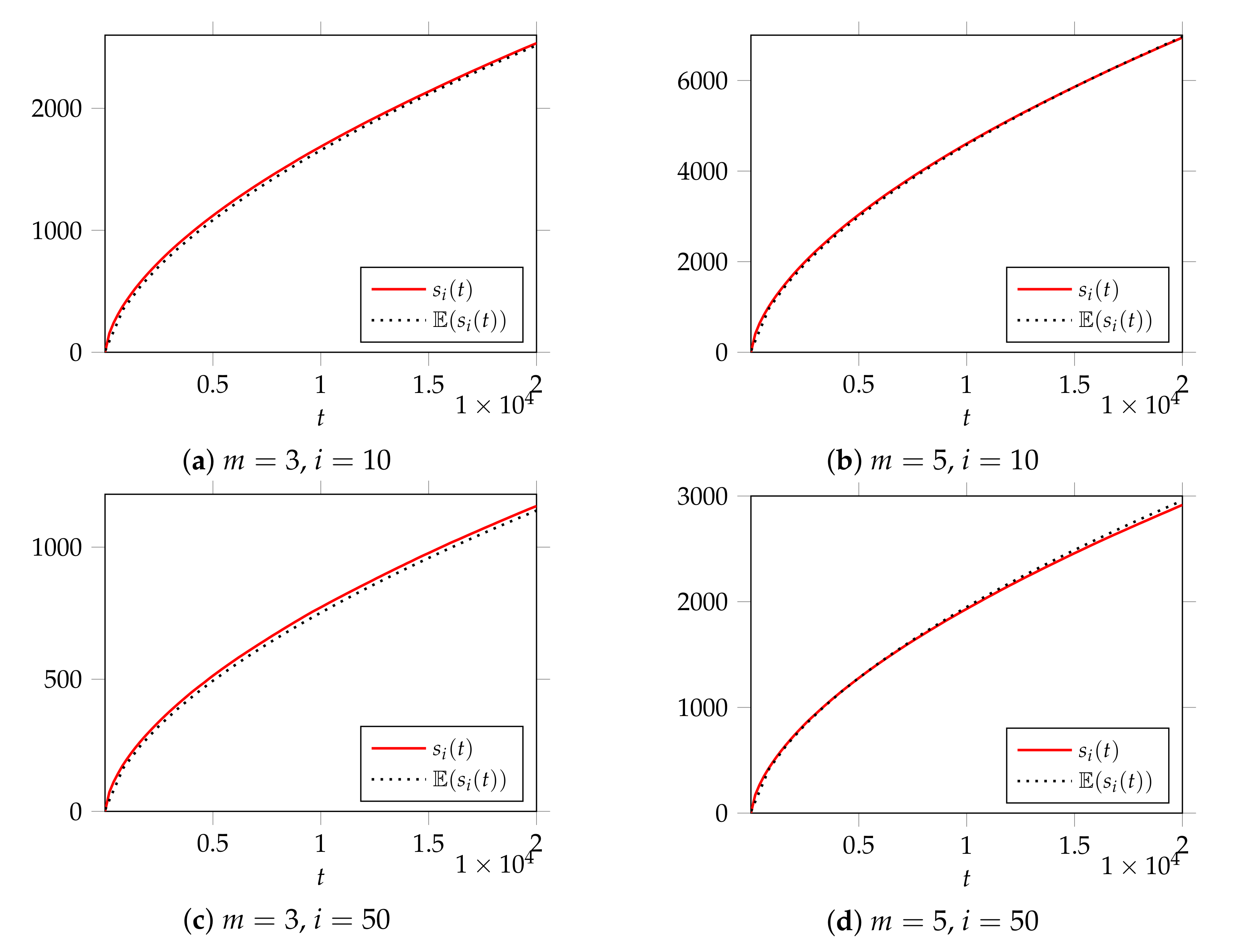
To exhibit the result, we carried out $T=200$ independent repetitions; in each of them the BA graph was simulated for $N=$ 20,000 iterations, for different values $m=3$ and $m=5$. Then the empirical values of $\mathrm{E}\left(s_i\left(t\right)\right)$ were obtained. The results are presented in Figure 9.

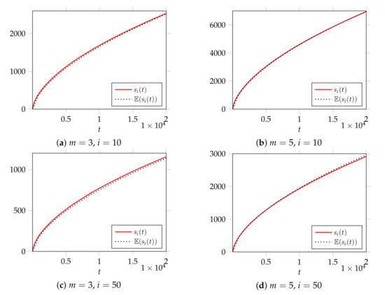
Figure 9. Dynamics of empiricalvalues for $\mathrm{Mean}\left(s_i\left(t\right)\right)$ in networks based on BA model for selected nodes $i=10,50$ as t iterates up to 20,000. The network in (a) is modeled with $m=3$, $i=10$, (b) with $m=5$, $i=10$, (c) with $m=3$, $i=50$, (d) with $m=5$, $i=50$.

Lemma 3.

The second moment of $s_i\left(t\right)$ is

$$\mathbb{E}\left(s_i^2\left(t\right)\right)=\frac{t}{i}\left(\frac{m^3(m+1)}{4}{log}^{2}t-m^{3}logt+m^2\left(\frac{(m+1){log}^{2}i}{4}-logi+1\right)\right).$$

Proof. 

Let us consider how the values $s_i(t+1)$ and $s_i\left(t\right)$ are related:

• If new vertex $v_{t+1}$ joins the vertex $v_i$ at the time $t+1$, then $s_i\left(t\right)$ increases by m, since the vertex i obtains a new neighbor whose degree is m;
• If new vertex $v_{t+1}$ joins one of the neighbors for vertex i, then $s_i\left(t\right)$ increases by 1, since in this case the contribution of one neighboring vertex to the increase of $s_i\left(t\right)$ is 1;
• If none of these events occurs, then $s_i\left(t\right)$ does not change.

Now we can obtain the stochastic difference equation for the random variable $s_i^2\left(t\right)$ at the moment of time t. We have

$$\begin{array}{c}\Delta s_i^2(t+1):=s_i^2(t+1)-s_i^2\left(t\right)=\hfill \\ {\xi }_i^{t+1}{(s_i\left(t\right)+m)}^2+{\eta }_i^{t+1}{(s_i\left(t\right)+1)}^2+(1-{\xi }_i^{t+1}-{\eta }_i^{t+1})s_i^2\left(t\right)-s_i^2\left(t\right)=\\ \hfill {\xi }_i^{t+1}(2m{s}_i\left(t\right)+m^2)+{\eta }_i^{t+1}(2s_i\left(t\right)+1).\end{array}$$

(20)

Since

$$\mathbb{E}\left({\xi }_i^{t+1}\right|G_t)=\frac{d_i\left(t\right)}{2t},\mathbb{E}\left({\eta }_i^{t+1}\right|G_t)=\frac{s_i\left(t\right)}{2t},$$

(21)

we get

$$\mathbb{E}(\Delta s_i^2(t+1)|G_t)=\frac{s_i^2\left(t\right)}{t}+m\frac{d_i\left(t\right)s_i\left(t\right)}{t}+\frac{s_i\left(t\right)}{2t}+m^2\frac{d_i\left(t\right)}{2t}.$$

(22)

We cannot assert that $s_i\left(t\right)$ and $d_i\left(t\right)$ are independent; therefore, we may expect that $\mathbb{E}\left(d_i\left(t\right)s_i\left(t\right)\right)\ne \mathbb{E}\left(d_i\left(t\right)\right)\mathbb{E}\left(s_i\left(t\right)\right)$. Lemma A1 finds $\mathbb{E}\left(d_i\left(t\right)s_i\left(t\right)\right)$ (see Appendix A).

Using Lemma A1, Equations (2) and (19), passing to the mathematical expectation of both sides, and making the substitution $f=\mathbb{E}\left(s_i^2\left(t\right)\right|G_t)$ for convenience, we get the approximate differential equation:

$$\frac{df}{dt}=\frac{f}{t}+\frac{m^3(m+1)}{2i}logt-\frac{m^3}{i}.$$

(23)

Its solution has the form

$$f\left(t\right)=\frac{m^3(m+1)t}{4i}{log}^{2}t-\frac{m^{3}t}{i}logt+Ct,$$

where C is a constant. We have

$$\mathbb{E}\left(s_i^2\left(i\right)\right)=\frac{m^3(m+1)}{4}{log}^{2}i-m^{3}logi+Ci.$$

(24)

On the other hand, since $\mathbb{E}\left(s_i\left(i\right)\right)=\frac{m}{2}((m+1)logi-2)$, we have

$$\mathbb{E}\left(s_i^2\left(i\right)\right)=\frac{m^2{(m+1)}^2}{4}{log}^{2}i-m^2(m+1)logi+m^2.$$

(25)

Equating this result with (24), we find C:

$$C=\frac{1}{4i}{m}^2(m+1){log}^{2}i-\frac{m^2}{i}logi+\frac{m^2}{i}.$$

Thus, we get Lemma. □

To confirm the result, we carried out $T=200$ independent repetitions; in each of them the BA graph was simulated for $N=$ 20,000 iterations, for different values $m=3$ and $m=5$. Then, the empirical values of $\mathrm{mean}\left(s_i^2\left(t\right)\right)$ were obtained. The results are presented in Figure 10.

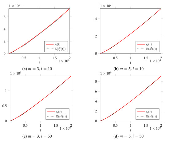
Figure 10. Dynamics of empirical values for $\mathrm{Mean}\left(s_i^2\left(t\right)\right)$ in networks based on BA model for selected nodes $i=10,50$ as t iterates up to 20,000. Network in (a) is modeled with $m=3$, $i=10$, (b) with $m=5$, $i=10$, (c) with $m=3$, $i=50$, (d) with $m=5$, $i=50$.

Theorem 5.

The variation of $s_i\left(t\right)$ follows

$$\mathrm{Var}\left(s_i\left(t\right)\right)=\mathbb{E}\left(s_i^2\left(t\right)\right)-{\mathbb{E}}^2\left(s_i\left(t\right)\right)=\frac{m^3}{4}\left({log}^2\frac{t}{i}-6logilogt\right)\frac{t}{i}.$$

Proof. 

Since $\mathrm{Var}\left(s_i\left(t\right)\right)=\mathbb{E}\left(s_i^2\left(t\right)\right)-{\mathbb{E}}^2\left(s_i\left(t\right)\right)$, the statement is the consequence of Equation (19) and Lemma 3. □

4.2. The Third Moment and the Asymmetry Coefficient of $s_i\left(t\right)$

Lemma 4.

The third moment of $s_i\left(t\right)$ is

$$\mathbb{E}\left(s_i^3\left(t\right)\right)=\frac{1}{8}{m}^4(m+1)(m+2){\left(\frac{t}{i}\right)}^{\frac{3}{2}}{log}^{3}t+O\left(t^{\frac{3}{2}}{log}^{2}t\right)$$

Proof. 

Let us obtain the difference stochastic equation describing the dynamics of random variable $s_i^3\left(t\right)$ at moment t. We have

$$\begin{array}{c}\Delta s_i^3(t+1):=s_i^3(t+1)-s_i^3\left(t\right)=\hfill \\ {\xi }_i^{t+1}{(s_i\left(t\right)+m)}^3+{\eta }_i^{t+1}{(s_i\left(t\right)+1)}^3+(1-{\xi }_i^{t+1}-{\eta }_i^{t+1})s_i^3\left(t\right)-s_i^3\left(t\right)=\\ \hfill {\xi }_i^{t+1}(3m{s}_i^2\left(t\right)+3m^2{s}_i\left(t\right)+m^3)+{\eta }_i^{t+1}(3s_i^2+3s_i\left(t\right)+1).\end{array}$$

(26)

It follows from (21) that

$$\begin{array}{c}\mathbb{E}(\Delta s_i^3(t+1)|G_t)=\hfill \\ \hfill \frac{3s_i^3\left(t\right)}{2t}+3m\frac{d_i\left(t\right)s_i^2\left(t\right)}{2t}+\frac{3s_i^2\left(t\right)}{2t}+3m^2\frac{s_i\left(t\right)d_i\left(t\right)}{2t}+\frac{s_i\left(t\right)}{2t}+m^3\frac{d_i\left(t\right)}{2t}.\end{array}$$

(27)

Note that $s_i\left(t\right)$ and $d_i\left(t\right)$ may not be independent, and therefore, it is possible that $\mathbb{E}\left(d_i\left(t\right)s_i^2\left(t\right)\right)\ne \mathbb{E}\left(d_i\left(t\right)\right)\mathbb{E}\left(s_i^2\left(t\right)\right)$.

After using Lemma A3, Lemma A1, Lemma 3, and Equations (19) and (2), taking the expectation of both parts, making the substitution $f=\mathbb{E}\left(s_i^2\left(t\right)\right)$, we get

$$\frac{df}{dt}=\frac{3f}{2t}+\frac{3}{8}{m}^4(m+1)(m+2)\frac{t^{\frac{1}{2}}}{i^{\frac{3}{2}}}{log}^{2}t+O(t^{\frac{1}{2}}logt),$$

(28)

The solution of which is

$$f\left(t\right)=\frac{1}{8}{m}^4(m+1)(m+2){\left(\frac{t}{i}\right)}^{\frac{3}{2}}{log}^{3}t+O\left(t^{\frac{3}{2}}{log}^{2}t\right).$$

□

To confirm the result, we carried out $T=200$ independent repetitions, and in each of them, the BA graph was simulated for $N=$ 20,000 iterations, for different values $m=3$ and $m=5$. Then the empirical values of $\mathrm{mean}\left(s_i^3\left(t\right)\right)$ were obtained. The results are presented in Figure 11.

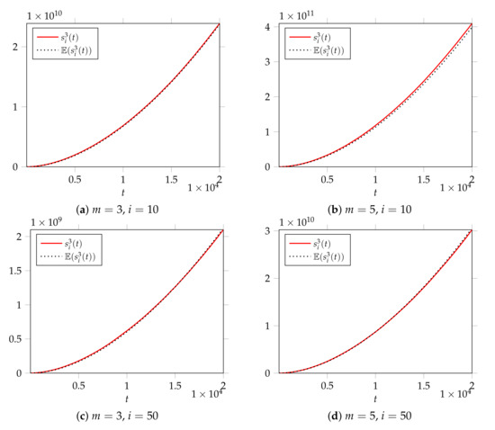
Figure 11. Dynamics of empirical values for $\mathrm{Mean}\left(s_i^3\left(t\right)\right)$ in networks based on BA model for selected nodes $i=10,50$ as t iterates up to $20,000$. Network in (a) is modeled with $m=3$, $i=10$, (b) with $m=5$, $i=10$, (c) with $m=3$, $i=50$, (d) with $m=5$, $i=50$.

Theorem 6.

The asymmetry coefficient of $s_i\left(t\right)$ follows

$${\gamma }_1\left(s_i\left(t\right)\right)\sim \frac{2}{m^{\frac{1}{2}}}$$

for sufficiently large t.

Proof. 

The asymmetry coefficient ${\gamma }_1\left(s_i\left(t\right)\right)$ is defined by

$${\gamma }_1\left(s_i\left(t\right)\right)=\frac{{\mu }_3\left(s_i\left(t\right)\right)}{{\mu }_2^{3/2}\left(s_i\left(t\right)\right)},$$

(29)

where ${\mu }_3\left(s_i\left(t\right)\right)$ and ${\mu }_2\left(s_i\left(t\right)\right)$ are the third and the second central moments of the $s_i\left(t\right)$-distribution, respectively. It follows from Lemma 4, Lemma 3, and Equation (19) that

$${\mu }_3\left(s_i\left(t\right)\right)=\mathbb{E}\left(s_i^3\right)-3\mathbb{E}\left(s_i^2\right)\mathbb{E}\left(s_i\right)+2{\mathbb{E}}^3\left(s_i\right)=\frac{1}{4}{m}^4{\left(\frac{t}{i}\right)}^{\frac{3}{2}}{log}^{3}t+O\left(t^{\frac{3}{2}}{log}^{2}t\right).$$

(30)

From Lemma 3, we have

$$\begin{array}{c}{\mu }_2^{3/2}\left(s_i\left(t\right)\right)={\mathrm{Var}}^{3/2}\left(s_i\left(t\right)\right)=\frac{m^{\frac{9}{2}}}{8}{\left({log}^2\frac{t}{i}-6logilogt\right)}^{\frac{3}{2}}{\left(\frac{t}{i}\right)}^{\frac{3}{2}}=\hfill \\ \hfill \frac{m^{\frac{9}{2}}}{8}{\left(\frac{t}{i}\right)}^{\frac{3}{2}}{log}^{3}t+O\left(t^{\frac{3}{2}}{log}^{2}t\right).\end{array}$$

(31)

Theorem follows from (29)–(31). □

Remark 4.

The positivity of ${\gamma }_1\left(s_i\left(t\right)\right)$ implies the asymmetry of the distribution.

4.3. The Kurtosis of $s_i\left(t\right)$

Lemma 5.

The fourth moment of $s_i$ at moment t follows

$$\mathbb{E}\left(s_i^4\left(t\right)\right)\sim \frac{1}{16}{m}^5(m+1)(m+2)(m+3){\left(\frac{t}{i}\right)}^2{log}^{4}t+o\left(t^2{log}^{3}t\right)$$

Proof. 

The change in the value of $s_i^4\left(t\right)$ from t to $t+1$ occurs as follows:

$$\begin{array}{c}\Delta s_i^4(t+1):=s_i^4(t+1)-s_i^4\left(t\right)=\hfill \\ \xi {(s_i\left(t\right)+m)}^4+\eta d_i\left(t\right){(s_i\left(t\right)+1)}^4+(1-\xi -\eta )s_i^4\left(t\right)-s_i^4\left(t\right)=\\ \hfill \xi (4m{s}_i^3\left(t\right)+6m^2{s}_i^2\left(t\right)+4m^3{s}_i\left(t\right)+m^4)+\eta (4s_i^3\left(t\right)+6s_i^2\left(t\right)+4s_i\left(t\right)+1).\end{array}$$

Equation (21) implies that

$$\begin{array}{c}\mathbb{E}(\Delta s_i^4(t+1)\mid G_t)=\hfill \\ \frac{2s_i^4\left(t\right)}{t}+\frac{2m{d}_i\left(t\right)s_i^3\left(t\right)}{t}+\frac{3s_i^3\left(t\right)}{t}+\frac{3m^2{d}_i\left(t\right)s_i^2\left(t\right)}{t}+\frac{2s_i^2\left(t\right)}{t}+\frac{2m^3{d}_i\left(t\right)s_i\left(t\right)}{t}+\\ \hfill \frac{2s_i^2\left(t\right)}{t}+\frac{s_i\left(t\right)}{2t}+\frac{m^4{d}_i\left(t\right)}{2t}.\end{array}$$

Denote $f\left(t\right)=\mathbb{E}\left(d_i\left(t\right)s_i^3\left(t\right)\right)$. Using Equations (2) and (19), Lemmas 3, 4, A1, A3, A4, and A6, we get the following differential equation

$$\frac{df\left(t\right)}{dt}=\frac{2f\left(t\right)}{t}+\frac{1}{4}{m}^5(m+1)(m+2)(m+3)\frac{t}{i^2}{log}^{3}t+O\left(t{log}^{2}t\right),$$

the solution of which has the form

$$f\left(t\right)=\frac{1}{16}{m}^5(m+1)(m+2)(m+3){\left(\frac{t}{i}\right)}^2{log}^{4}t+O\left(t^2{log}^{3}t\right).$$

□

Theorem 7.

The Kurtosis of $s_i\left(t\right)$ at iteration t follows

$$\mathrm{Kurt}\left(s_i\left(t\right)\right)=\frac{{\mu }_4\left(s_i\left(t\right)\right)}{{\mathrm{Var}}^2\left(s_i\left(t\right)\right)}\sim \frac{3(m+2)}{m}$$

for sufficiently large t.

Proof. 

By definition, we have

$$\begin{array}{c}{\mu }_4\left(s_i\left(t\right)\right)=\mathbb{E}\left(s_i^4\left(t\right)\right)-4\mathbb{E}\left(s_i\left(t\right)\right)\mathbb{E}\left(s_i^3\left(t\right)\right)+6{\mathbb{E}}^2\left(s_i\left(t\right)\right)\mathbb{E}\left(s_i^2\left(t\right)\right)-3{\mathbb{E}}^4\left(s_i\left(t\right)\right)=\hfill \\ \frac{1}{16}{m}^5(m+1)(m+2)(m+3){\left(\frac{t}{i}\right)}^2{log}^{4}t-\\ 4·\frac{m^2}{2}{\left(\frac{t}{i}\right)}^{1/2}logt·\frac{1}{8}{m}^4(m+1)(m+2){\left(\frac{t}{i}\right)}^{3/2}{log}^{3}t+\\ 6·\frac{m^4}{4}\frac{t}{i}{log}^{2}t·\frac{t}{i}\frac{m^3(m+1)}{4}{log}^{2}t-3\frac{m^8}{16}{\left(\frac{t}{i}\right)}^2{log}^{4}t+O\left(t^2{log}^{3}t\right)=\\ \hfill \frac{3}{16}{m}^5(m+2){\left(\frac{t}{i}\right)}^2{log}^{4}t+o\left(t^2{log}^{3}t\right).\end{array}$$

It follows from Theorem 5 that

$${\mathrm{Var}}^2\left(s_i\left(t\right)\right)=\frac{m^6}{16}{\left(\frac{t}{i}\right)}^2{log}^{4}t+o\left(t^2{log}^{3}t\right).$$

Therefore,

$$\mathrm{Kurt}\left(s_i\left(t\right)\right)\sim \frac{3(m+2)}{m}$$

for large t. □

5. Conclusions

In this article, we studied two Markov non-stationary random processes related to the evolution of BA networks: the first of them describes the dynamics of the degree of one fixed network node, the second is related to the dynamics of the total degree of the neighbors of one node. We evaluated the dynamic behavior of some characteristics of the distributions of these two random variables, which are associated with higher-order moments, including their variation, skewness, and kurtosis. The analysis showed that both distributions have the following properties:

• The coefficient of variation, defined as the ratio of the mathematical expectation to the variance, is close to the value of $\sqrt{\frac{m+1}{m}}$ at each moment of time. Moreover, as the number of iterations increases, the coefficient of variation converges to $\sqrt{\frac{m+1}{m}}$.
• The skewness coefficient is positive for both distributions at any moment of the network evolution, which indicates that both distributions are asymmetric (their right tails are greater than their left ones).
• The kurtosis is greater than 3 for all subsequent iterations. This means that the right tails of both distributions are thicker than the tail of the normal distribution.
• It is also interesting to note that if the number of added edges m increases, then the coefficient of variation approaches 1, the coefficient of asymmetry tends to 0, and kurtosis converges to 3. This means that the characteristics of the random numbers are close to the ones of the normal distribution.

It should also be noted that although the characteristics of both distributions are close to each other, the mathematical expectation of the total degree of the neighbors of a node grows $logt$ times faster than the expected degree of the same node.

References

- Lieberman, M.B.; Montgomery, D.B. First-mover advantages. Strateg. Manag. J. 1988, 9, 41–58. [Google Scholar] [CrossRef]
- Faloutsos, M.; Faloutsos, P.; Faloutsos, C. On Power-Law Relationships of the Internet Topology. SIGCOMM Comput. Commun. Rev. 1999, 29, 251–262. [Google Scholar] [CrossRef]
- Kleinberg, J.M.; Kumar, R.; Raghavan, P.; Rajagopalan, S.; Tomkins, A.S. The Web as a Graph: Measurements, Models, and Methods. In International Computing and Combinatorics Conference; Asano, T., Imai, H., Lee, D.T., Nakano, S.I., Tokuyama, T., Eds.; Springer: Berlin/Heidelberg, Germany, 1999; pp. 1–17. [Google Scholar] [CrossRef]
- Clauset, A.; Shalizi, C.R.; Newman, M.E.J. Power-Law Distributions in Empirical Data. SIAM Rev. 2009, 51, 661–703. [Google Scholar] [CrossRef] [Green Version]
- De Solla Price, D. Networks of scientific papers. Science 1976, 149, 292–306. [Google Scholar] [CrossRef] [PubMed]
- Klaus, A.; Yu, S.; Plenz, D. Statistical Analyses Support Power Law Distributions Found in Neuronal Avalanches. PLoS ONE 2011, 6, e19779. [Google Scholar] [CrossRef] [PubMed] [Green Version]
- Newman, M.E.J. The Structure and Function of Complex Networks. SIAM Rev. 2003, 45, 167–256. [Google Scholar] [CrossRef] [Green Version]
- Albert, R.; Barabási, A.L. Statistical mechanics of complex networks. Rev. Mod. Phys. 2002, 74, 47–97. [Google Scholar] [CrossRef] [Green Version]
- Barabási, A.L.; Albert, R. Emergence of Scaling in Random Networks. Science 1999, 286, 509–512. [Google Scholar] [CrossRef] [Green Version]
- Dorogovtsev, S.N.; Mendes, J.F.F.; Samukhin, A.N. Structure of growing networks with preferential linking. Phys. Rev. Lett. 2000, 85, 4633–4636. [Google Scholar] [CrossRef] [PubMed] [Green Version]
- Krapivsky, P.L.; Redner, S. Organization of growing random networks. Phys. Rev. E 2001, 63, 066123. [Google Scholar] [CrossRef] [Green Version]
- Krapivsky, P.L.; Redner, S.; Leyvraz, F. Connectivity of growing random networks. Phys. Rev. Lett. 2000, 85, 4629–4632. [Google Scholar] [CrossRef] [Green Version]
- Sidorov, S.; Mironov, S. Growth network models with random number of attached links. Phys. A Stat. Mech. Its Appl. 2021, 576, 126041. [Google Scholar] [CrossRef]
- Tsiotas, D. Detecting differences in the topology of scale-free networks grown under time-dynamic topological fitness. Sci. Rep. 2020, 10, 10630. [Google Scholar] [CrossRef]
- Pal, S.; Makowski, A.M. Asymptotic Degree Distributions in Large (Homogeneous) Random Networks: A Little Theory and a Counterexample. IEEE Trans. Netw. Sci. Eng. 2020, 7, 1531–1544. [Google Scholar] [CrossRef] [Green Version]
- Rak, R.; Rak, E. The fractional preferential attachment scale-free network model. Entropy 2020, 22, 509. [Google Scholar] [CrossRef] [PubMed]
- Cinardi, N.; Rapisarda, A.; Tsallis, C. A generalised model for asymptotically-scale-free geographical networks. J. Stat. Mech. Theory Exp. 2020, 2020, 043404. [Google Scholar] [CrossRef] [Green Version]
- Shang, K.K.; Yang, B.; Moore, J.M.; Ji, Q.; Small, M. Growing networks with communities: A distributive link model. Chaos 2020, 30, 041101. [Google Scholar] [CrossRef]
- Bertotti, M.L.; Modanese, G. The configuration model for Barabasi-Albert networks. Appl. Netw. Sci. 2019, 4, 1–13. [Google Scholar] [CrossRef] [Green Version]
- Pachon, A.; Sacerdote, L.; Yang, S. Scale-free behavior of networks with the copresence of preferential and uniform attachment rules. Phys. D Nonlinear Phenom. 2018, 371, 1–12. [Google Scholar] [CrossRef] [Green Version]
- Van Der Hofstad, R. Random Graphs and Complex Networks; Cambridge University Press: Cambridge, UK, 2016; Volume 1. [Google Scholar] [CrossRef] [Green Version]
- Barabási, A.; Albert, R.; Jeong, H. Mean-field theory for scale-free random networks. Phys. A Stat. Mech. Its Appl. 1999, 272, 173–187. [Google Scholar] [CrossRef] [Green Version]
- Krapivsky, P.L.; Redner, S. Finiteness and fluctuations in growing networks. J. Phys. A Math. Gen. 2002, 35, 9517–9534. [Google Scholar] [CrossRef]
- Kadanoff, L. More is the Same; Phase Transitions and Mean Field Theories. J. Stat. Phys. 2009, 137, 777–797. [Google Scholar] [CrossRef]
- Parr, T.; Sajid, N.; Friston, K.J. Modules or Mean-Fields? Entropy 2020, 22, 552. [Google Scholar] [CrossRef] [PubMed]
- Pachon, A.; Polito, F.; Sacerdote, L. On the continuous-time limit of the Barabási-Albert random graph. Appl. Math. Comput. 2020, 378, 125177. [Google Scholar] [CrossRef] [Green Version]
- Sidorov, S.; Mironov, S.; Malinskii, I.; Kadomtsev, D. Local Degree Asymmetry for Preferential Attachment Model. Stud. Comput. Intell. 2021, 944, 450–461. [Google Scholar] [CrossRef]
- Sidorov, S.P.; Mironov, S.V.; Grigoriev, A.A. Friendship paradox in growth networks: Analytical and empirical analysis. Appl. Netw. Sci. 2021, 6, 35. [Google Scholar] [CrossRef]
Publisher’s Note: MDPI stays neutral with regard to jurisdictional claims in published maps and institutional affiliations. |
© 2021 by the authors. Licensee MDPI, Basel, Switzerland. This article is an open access article distributed under the terms and conditions of the Creative Commons Attribution (CC BY) license (https://creativecommons.org/licenses/by/4.0/).