

A Self-Similar Approach to Study Nanofluid Flow Driven by a Stretching Curved Sheet
 , ,
, ,
Abstract
:1. Introduction
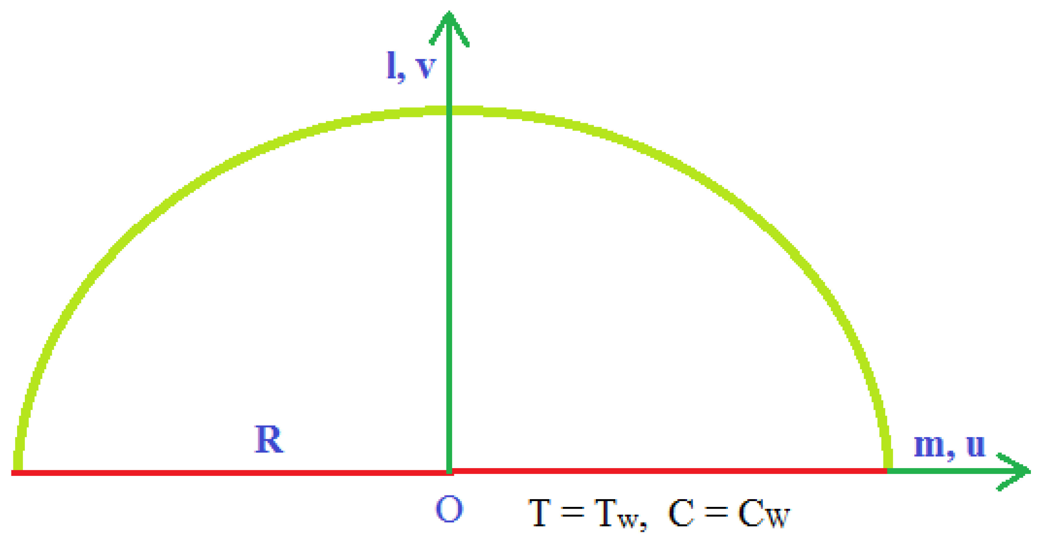
2. Mathematical Formulation
3. Computational Procedure
3.1. Quasi-Linearization Method
Procedure Steps
- (1)
- and are the initial guesses to assure the boundary conditions, which are specified in equation.
- (2)
- Set in Equation (28) to present the solution of the linear system.
- (3)
- We are solving a linear system by means of forgetting and .
- (4)
- By using new initial guesses that are and which converges to and , repeating this process to create sequences and
- (5)
- We are creating four sequences until
4. Results and Discussion
5. Conclusions
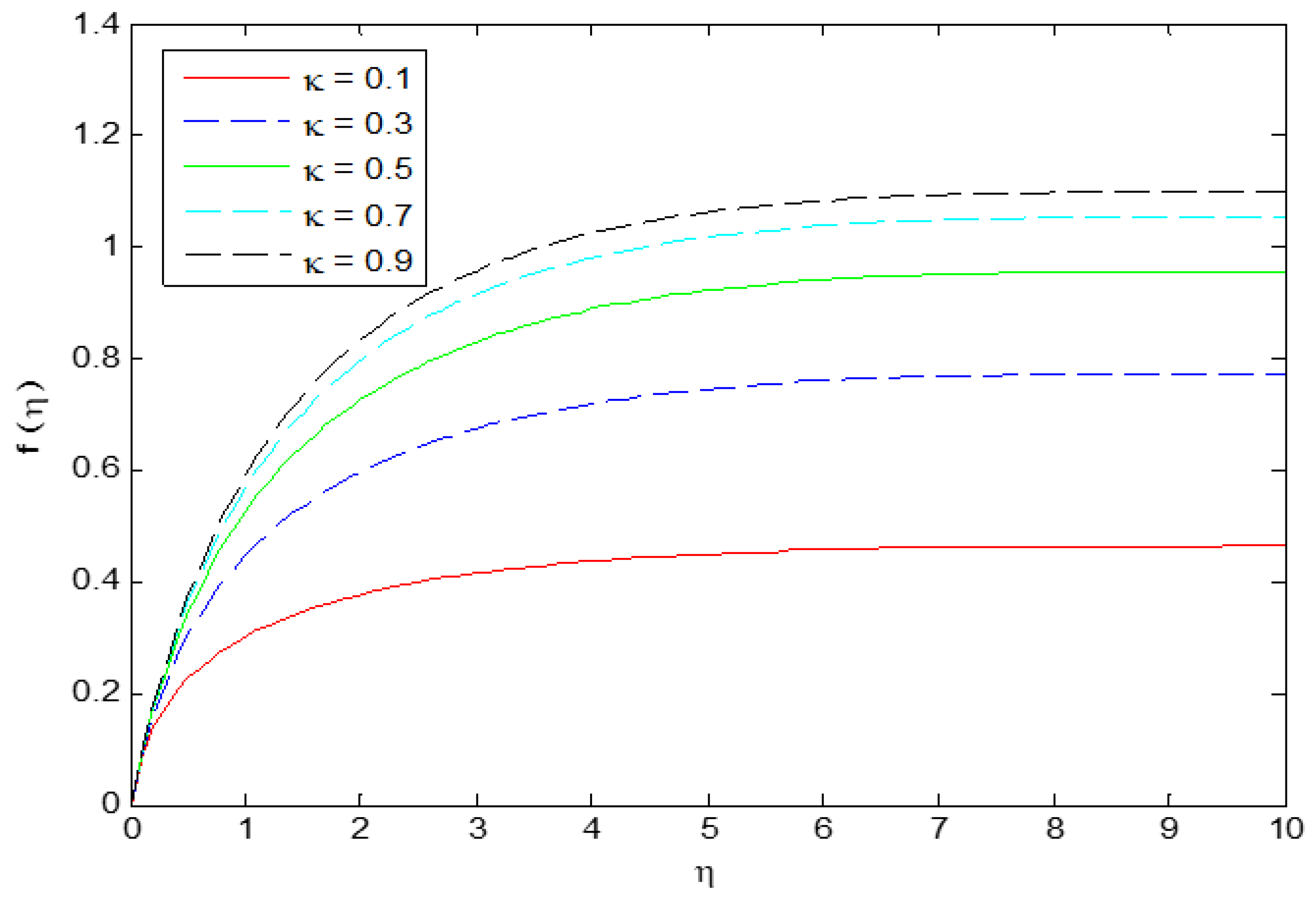
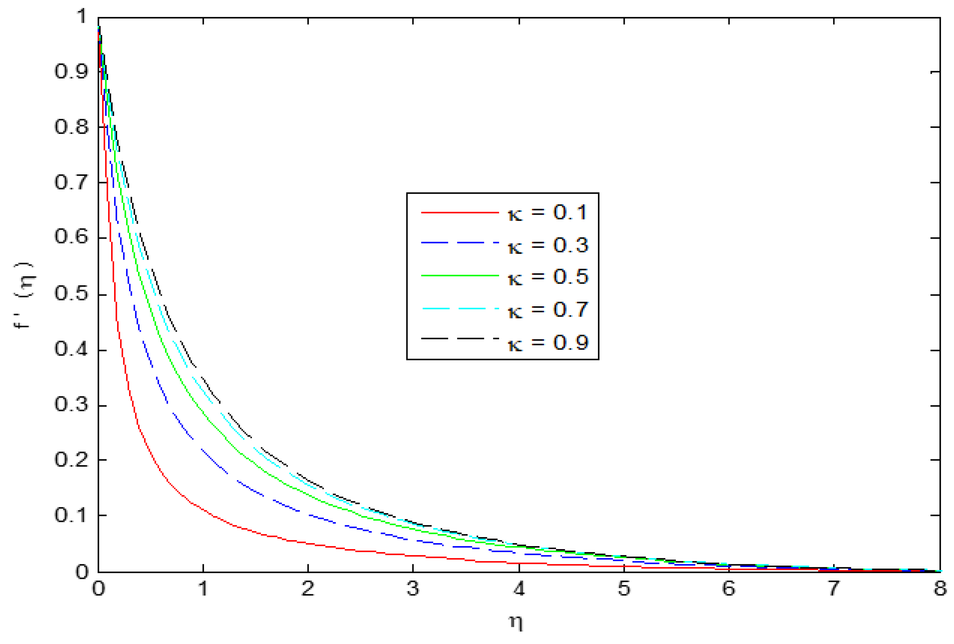
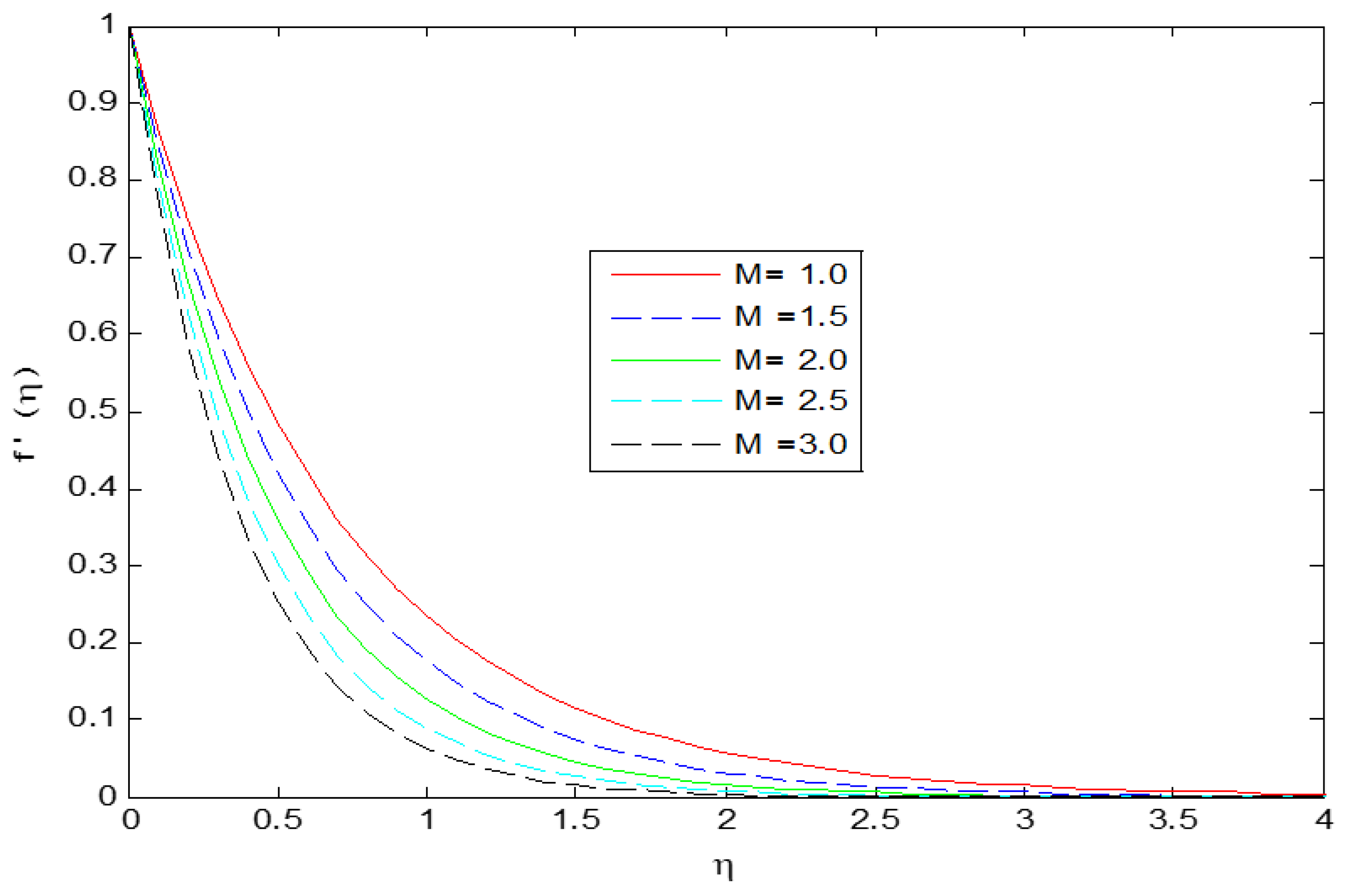
- Velocity profiles have shown enhancing behavior for higher values of while decreasing for magnetic parameter .
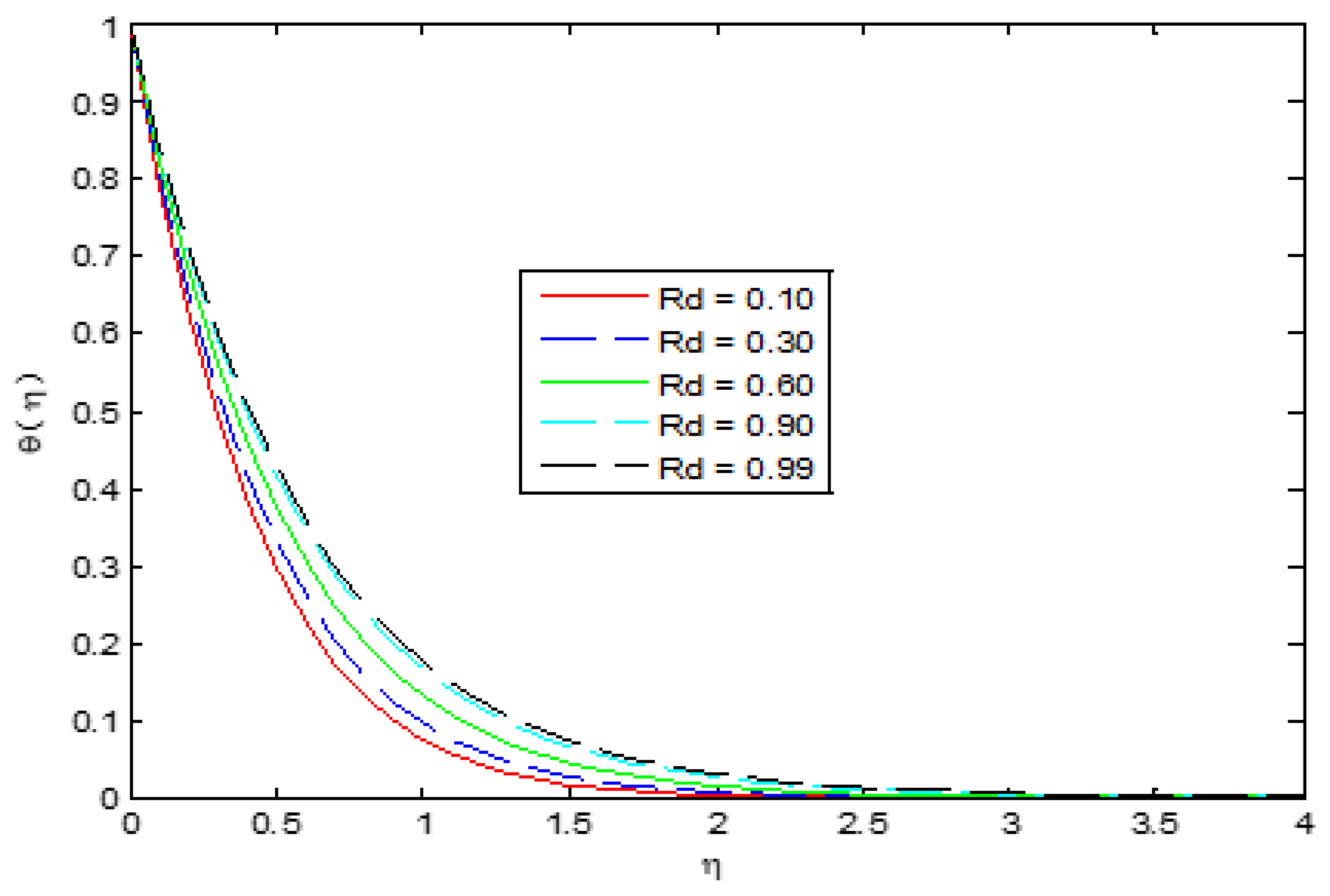
- Temperature profile enhances greater values of .
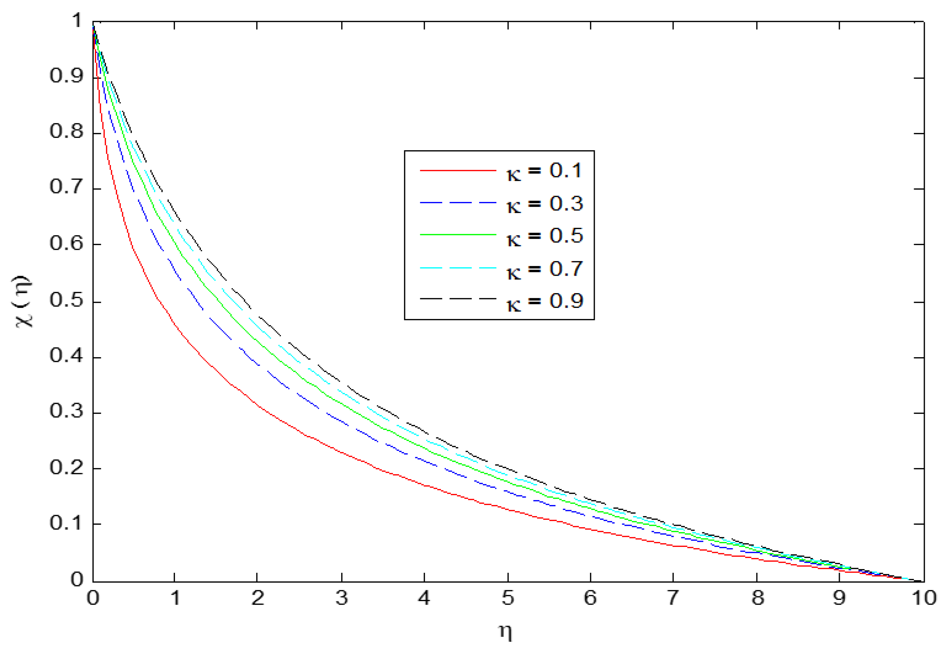
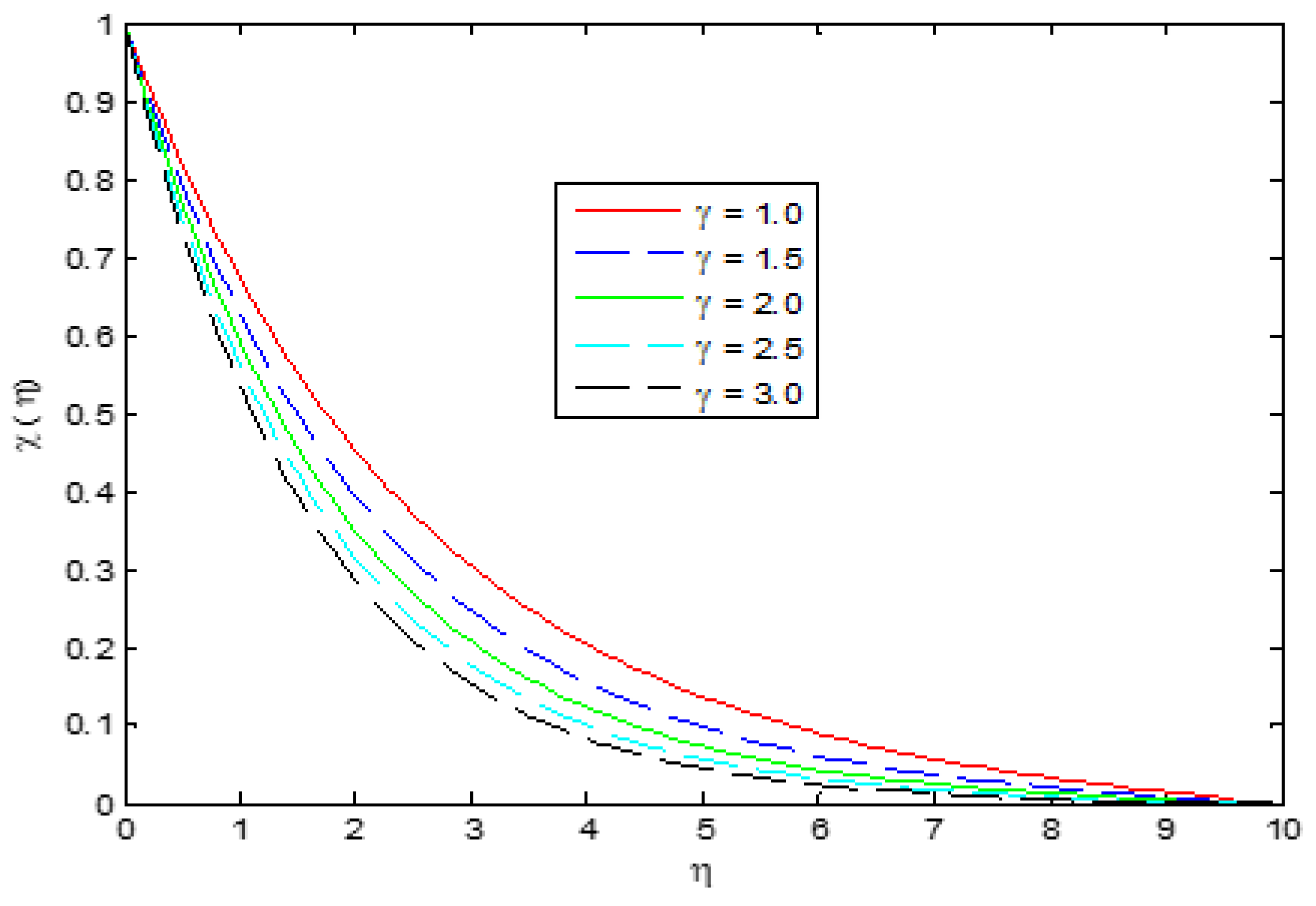
- Skin friction reduces for larger values of chemical reaction parameter .
- The Prandtl number tends to reduce the rate of heat transfer.
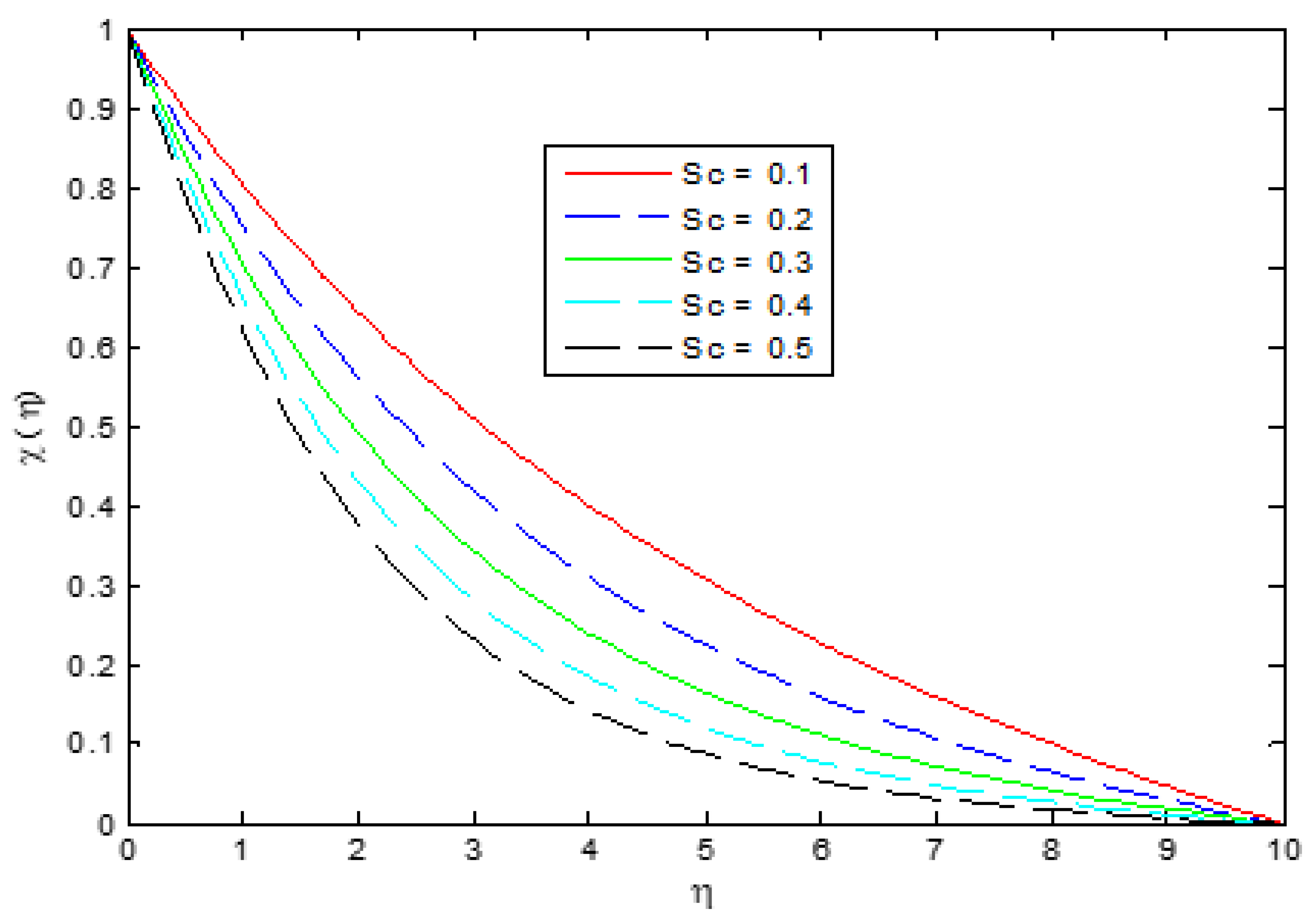
- The Schmidt number causes an increase in concentration.
Author Contributions
Funding
Institutional Review Board Statement
Informed Consent Statement
Data Availability Statement
Conflicts of Interest
Nomenclature
| Cartesian coordinates, [m] | |
| Velocity components, [ms−1] | |
| Specific heat, [] | |
| p | Pressure, [] |
| Thermal conductivity of the nano-fluid, [] | |
| T | Temperature, [K] |
| Greek Symbols | |
| Dynamic viscosity, [Nsm−2] | |
| Density, [kgm−3] | |
| Kinematics viscosity, [] | |
| Heat capacitance of the nano-fluid, [] | |
References
- Naveed, M.; Abbas, Z.; Sajid, M. MHD flow of Micropolar fluid due to a curved stretching sheet with thermal radiation. J. Appl. Fluid Mech. 2016, 9, 131–138. [Google Scholar] [CrossRef]
- Misra, J.C.; Shit, G.C.; Rath, H.J. Flow and heat transfer of a MHD viscoelastic fluid in a channel with stretching walls: Some application to hemodynamic. J. Sci. Direct 2008, 37, 1–11. [Google Scholar] [CrossRef]
- Abass, Z.; Naveed, M.; Sajid, M. Heat transfer analysis for a curved stretching flow over a curved surface with magnetic field. J. Eng. Thermophys. 2013, 22, 337–345. [Google Scholar] [CrossRef]
- Abbas, Z.; Sheikh, M.; Sajid, M. Hydrodynamic stagnation point flow of a micro polar viscoelastic fluid towards a stretching/shrinking sheet in the presence of heat generation. Can. J. Phys. 2014, 92, 1113–1123. [Google Scholar] [CrossRef]
- Hayyat, T.; Abbas, Z.; Javad, T. Mixed convention flow of a micropolar fluid over a non-linear stretching sheet. Phys. Lett. A 2008, 372, 637–647. [Google Scholar] [CrossRef]
- Hayyat, T.; Qasim, M. Effect of thermal radiation on unsteady magnetohydrodynamics flow of micropolar fluid with heat and mass transfer. J. Nat. 2010, 65, 950–960. [Google Scholar] [CrossRef]
- Kanti, P.K.; Sharma, K.V.; Said, Z.; Gupta, M. Experimental investigation on thermo-hydraulic performance of water-based fly ash–Cu hybrid nanofluid flow in a pipe at various inlet fluid temperatures. Int. Commun. Heat Mass Transf. 2021, 124, 105238. [Google Scholar] [CrossRef]
- Kanti, P.; Sharma, K.V.; Ramachandra, C.G.; Gupta, M. Thermal performance of fly ash nanofluids at various inlet fluid temperatures: An experimental study. Int. Commun. Heat Mass Transf. 2022, 119, 104926. [Google Scholar] [CrossRef]
- Bazdar, H.; Toghraie, D.; Pourfattah, F.; Akbari, O.A.; Nguyen, H.M.; Asadi, A. Numerical investigation of turbulent flow and heat transfer of nanofluid inside a wavy microchannel with different wavelengths. J. Therm. Anal. Calorim. 2020, 139, 2365–2380. [Google Scholar] [CrossRef]
- Sarlak, R.; Yousefzadeh, S.; Akbari, O.A.; Toghraie, D.; Sarlak, S.; Assadi, F. The investigation of simultaneous heat transfer of water/Al2O3 nanofluid in a close enclosure by applying homogeneous magnetic field. Int. J. Mech. Sci. 2017, 133, 674–688. [Google Scholar] [CrossRef]
- Ishak, A.; Nazar, R.; Pop, I. Heat transfer over a unsteady Stretching permeable surface with prescribe wall temperature, Non-linear analysis. Nonlinear Anal. Real World Appl. 2009, 10, 2909–2913. [Google Scholar] [CrossRef]
- Javad, T.; Ahmad, I.; Abass, Z.; Hayyat, T. Rotating flow of micropolar fluid induced by a stretching Surface. Z. Für Nat. A 2010, 65, 829–836. [Google Scholar] [CrossRef]
- Rasool, G.; Saeed, A.M.; Lare, A.I.; Abderrahmane, A.; Guedri, K.; Vaidya, H. Darcy-Forchheimer Flow of Water Conveying Multi-Walled Carbon Nanoparticles through a Vertical Cleveland Z-Staggered Cavity Subject to Entropy Generation. Micromachines 2022, 13, 744. [Google Scholar] [CrossRef] [PubMed]
- Rasool, G.; Shafiq, A.; Hussain, S.; Zaydan, M.; Wakif, A.; Chamkha, A.J.; Bhutta, M.S. Significance of Rosseland’s Radiative Process on Reactive Maxwell Nanofluid Flows over an Isothermally Heated Stretching Sheet in the Presence of Darcy-Forchheimer and Lorentz Forces: Towards a New Perspective on Buongiorno’s Model. Micromachines 2022, 13, 368. [Google Scholar] [CrossRef] [PubMed]
- Kumar, L. Finite element analysis of combined heat and mass transfer in hydro magnetic micro polar flow along a stretching sheet. Comput. Mater. Sci. 2009, 46, 841–848. [Google Scholar] [CrossRef]
- Mahmood, M.A.A.; Waheed, S.E. MHD flow and heat transfer of a micropolar fluid over a stretching surface with heat generation (absorption) and slip velocity. J. Egypt. Math. Soc. 2012, 20, 20–27. [Google Scholar] [CrossRef]
- Makinde, O.D. Similarity solution of hydromagnetic heat and mass transfer over a vertical plate with a convective surface boundary condition. Int. J. Phys. Sci. 2010, 5, 20–27. [Google Scholar]
- Nazar, R.; Amin, N.; Filip, D.; Pop, I. Stagnation point flow of a micropolar fluid towards a stretching sheet. Int. J. Non-linear Mech. 2004, 39, 1227–1235. [Google Scholar] [CrossRef]
- Sajid, M.; Ali, N.; Javed, T.; Abbas, Z. Stretching a curved surface in a various fluids. Chin. Phys. Lett. 2010, 27, 024703. [Google Scholar] [CrossRef]
- Sajid, M.; Ali, N.; Javed, T.; Abbas, Z. Flow of a micropolar fluid over a curved stretching surface. J. Eng. Phys. 2011, 84, 864–871. [Google Scholar] [CrossRef]
- Raju, C.S.K.; Sandeep, N.; Sugunamma, V.; JayachandraBabu, M.; Reddy, J.V.R. Heat and mass transfer in magneto-hydrodynamic casson fluid over an exponentially permeable stretching surface. Eng. Sci. Technol. Int. J. 2016, 19, 45–52. [Google Scholar]
- Reddy, P.B. Magneto-hydrodynamic Flow of a Casson Fluid over an Exponentially Inclined Permeable Stretching Surface with Thermal Radiation and Chemical Reaction. Ain Shams Eng. J. 2016, 7, 593–602. [Google Scholar] [CrossRef] [Green Version]
- Ibrahim, S.M.; Lorenzini, G.; Kumar, P.V.; Raju, C.S.K. Influence of chemical reaction and heat source on dissipative MHD mixed convection flow of a Casson nanofluid over a nonlinear permeable strecting sheet. Int. J. Heat Mass Transf. 2017, 111, 346–355. [Google Scholar] [CrossRef]
- Ghadikolaei, S.S.; Hosseinzadeh, K.; Yassari, M.; Sadeghi, H.; Ganji, D.D. Boundary layer analysis of micropolar dusty fluid with TiO2 nanoparticles in a porous medium under the effect of magnetic field and thermal radiation over a stretching sheet. J. Mol. Liq. 2017, 244, 374–389. [Google Scholar] [CrossRef]
- Khan, I.; Malik, M.Y.; Salahuddin, T.; Khan, M.; Rehman, K.U. Homogenous–heterogeneous reactions in MHD flow of Powell–Eyring fluid over a stretching sheet with Newtonian heating. Neural Comput. Appl. 2018, 30, 3581–3588. [Google Scholar] [CrossRef] [PubMed]
- Nasir, S.; Islam, S.; Gul, T.; Shah, Z.; Khan, M.A.; Khan, W.; Khan, A.Z.; Khan, S. Three-dimensional rotating flow of MHD single wall carbon nanotubes over a stretching sheet in presence of thermal radiation. Appl. Nanosci. 2018, 8, 1361–1378. [Google Scholar] [CrossRef]
- Khan, N.S.; Islam, S.; Gul, T.; Khan, I.; Khan, W.; Ali, L. Thin film flow of a second grade fluid in a porous medium past a stretching sheet with heat transfer. Alex. Eng. J. 2018, 57, 1019–1031. [Google Scholar] [CrossRef]
- Khan, S.A.; Nie, Y.; Ali, B. Multiple slip effects on magnetohydrodynamic axisymmetric buoyant nanofluid flow above a stretching sheet with radiation and chemical reaction. Symmetry 2019, 11, 1171. [Google Scholar] [CrossRef]
- Mabood, F.; Imtiaz, M.; Hayat, T. Features of Cattaneo-Christov heat flux model for Stagnation point flow of a Jeffrey fluid impinging over a stretching sheet: A numerical study. Heat Transf. 2020, 49, 2706–2716. [Google Scholar] [CrossRef]
- Akbar, M.Z.; Ashraf, M.; Iqbal, M.F.; Ali, K. Heat and mass transfer analysis of unsteady MHD nano-fluid flow through a channel with moving porous walls and medium. AIP Adv. 2016, 6, 045222. [Google Scholar] [CrossRef]
- Hady, F.; Ibrahim, F.; El-Hawery, H.; Abdelhady, A. Effects of suction/injection on natural convection boundary layer flow of a nano-fluid past a vertical porous plate through a porous medium. J. Mod. Methods Numer. Math. 2012, 3, 53–63. [Google Scholar] [CrossRef]
- Ahmad, S.; Ali, K.; Saleem, R.; Bashir, H. Thermal Analysis of nano-fluid flow due to rotating cone/plate—A numerical study. AIP Adv. 2020, 10, 075024. [Google Scholar] [CrossRef]
- Iqbal, M.F.; Ahmad, S.; Ali, K.; Akbar, M.Z.; Ashraf, M. Analysis of heat and mass transfer in unsteady nanofluid flow between moving disks with chemical reaction—A Numerical Study. Heat Transf. Res. 2018, 49, 1403–1418. [Google Scholar] [CrossRef]
- Kanti, P.K.; Sharma, K.V.; Minea, A.A.; Kesti, V. Experimental and computational determination of heat transfer, entropy generation and pressure drop under turbulent flow in a tube with fly ash-Cu hybrid nanofluid. Int. J. Therm. Sci. 2021, 167, 107016. [Google Scholar] [CrossRef]
- Kanti, P.; Sharma, K.V.; Said, Z.; Bellos, E. Numerical study on the thermo-hydraulic performance analysis of fly ash nanofluid. J. Therm. Anal. Calorim. 2022, 147, 2101–2113. [Google Scholar] [CrossRef]
- Ruhani, B.; Barnoon, P.; Toghraie, D. Statistical investigation for developing a new model for rheological behavior of Silica–ethylene glycol/Water hybrid Newtonian nanofluid using experimental data. Phys. A Stat. Mech. Its Appl. 2019, 525, 616–627. [Google Scholar] [CrossRef]
- Mashayekhi, R.; Khodabandeh, E.; Akbari, O.A.; Toghraie, D.; Bahiraei, M.; Gholami, M. CFD analysis of thermal and hydrodynamic characteristics of hybrid nanofluid in a new designed sinusoidal double-layered microchannel heat sink. J. Therm. Anal. Calorim. 2018, 134, 2305–2315. [Google Scholar] [CrossRef]
- Arasteh, H.; Mashayekhi, R.; Goodarzi, M.; Motaharpour, S.H.; Dahari, M.; Toghraie, D. Heat and fluid flow analysis of metal foam embedded in a double-layered sinusoidal heat sink under local thermal non-equilibrium condition using nanofluid. J. Therm. Anal. Calorim. 2019, 138, 1461–1476. [Google Scholar] [CrossRef]
- Zari, I.; Shafiq, A.; Rasool, G.; Sindhu, T.N.; Khan, T.S. Double-stratified Marangoni boundary layer flow of Casson nanoliquid: Probable error application. J. Therm. Anal. Calorim. 2022, 147, 6913–6929. [Google Scholar] [CrossRef]
- Shafiq, A.; Mebarek-Oudina, F.; Sindhu, T.N.; Rasool, G. Sensitivity analysis for Walters-B nanoliquid flow over a radiative Riga surface by RSM. Sci. Iran. 2022, 29, 1236–1249. [Google Scholar]
- Batool, S.; Rasool, G.; Alshammari, N.; Khan, I.; Kaneez, H.; Hamadneh, N. Numerical analysis of heat and mass transfer in micropolar nanofluids flow through lid driven cavity: Finite volume approach. Case Stud. Therm. Eng. 2022, 37, 102233. [Google Scholar] [CrossRef]
- Rasool, G.; Shafiq, A.; Khan, I.; Baleanu, D.; Sooppy Nisar, K.; Shahzadi, G. Entropy Generation and Consequences of MHD in Darcy–Forchheimer Nanofluid Flow Bounded by Non-Linearly Stretching Surface. Symmetry 2020, 12, 652. [Google Scholar] [CrossRef]
- Rasool, G.; Shafiq, A.; Alqarni, M.S.; Wakif, A.; Khan, I.; Bhutta, M.S. Numerical Scrutinization of Darcy-Forchheimer Relation in Convective Magnetohydrodynamic Nanofluid Flow Bounded by Nonlinear Stretching Surface in the Perspective of Heat and Mass Transfer. Micromachines 2021, 12, 374. [Google Scholar] [CrossRef]
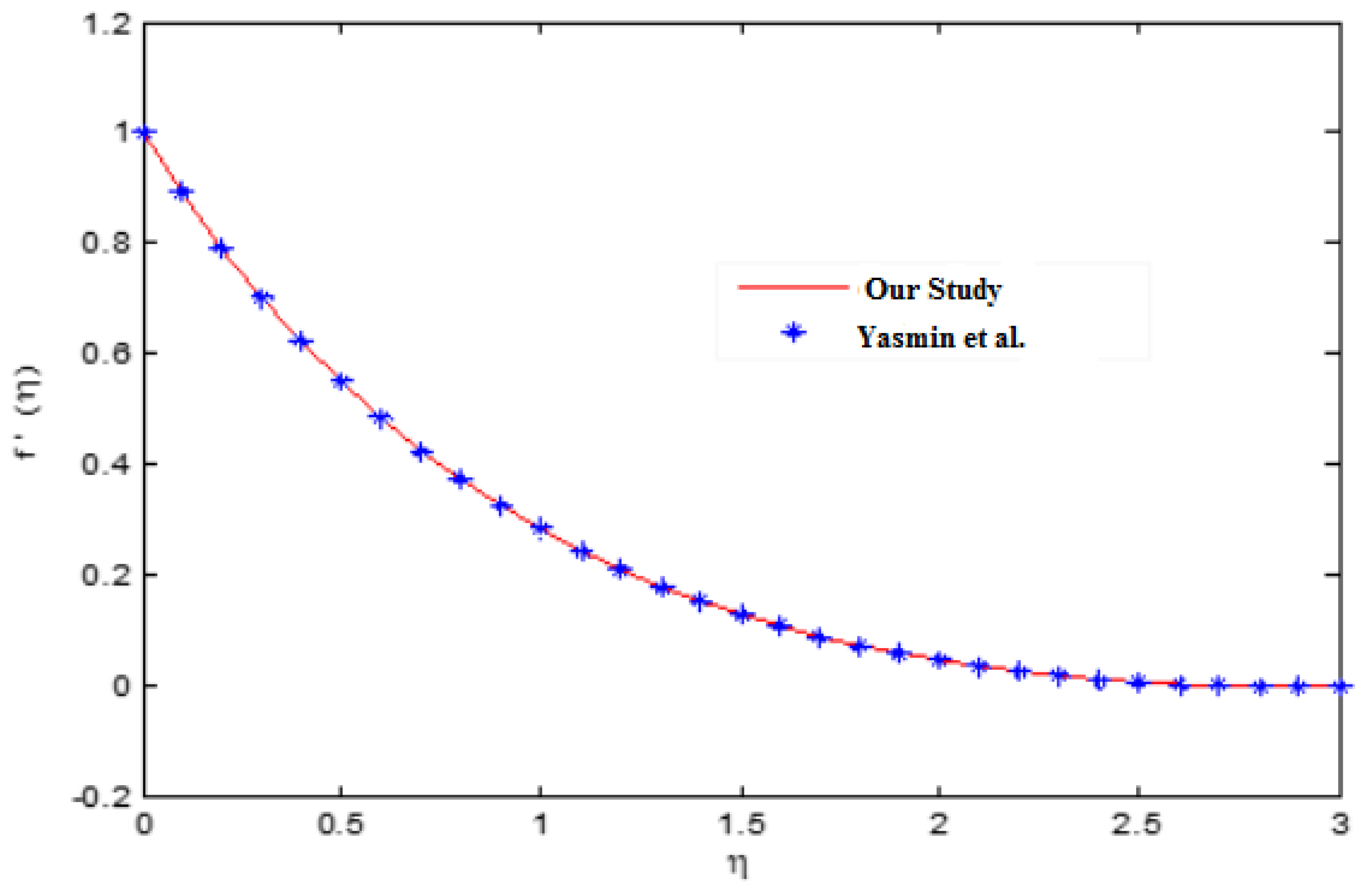
- Yasmin, A.; Ali, K.; Ashraf, M. Study of heat and mass transfer in MHD flow of micropolar fluid over a curved stretching sheet. Sci. Rep. 2020, 10, 4581. [Google Scholar] [CrossRef]
- Jamshed, W.; Aziz, A. Entropy Analysis of TiO2-Cu/EG Casson Hybrid Nanofluid via Cattaneo-Christov Heat Flux Model. Appl. Nanosci. 2018, 8, 1–14. [Google Scholar]
- Jamshed, W.; Nisar, K.S. Computational single phase comparative study of Williamson nanofluid in parabolic trough solar collector via Keller box method. Int. J. Energy Res. 2021, 45, 10696–10718. [Google Scholar] [CrossRef]
- Jamshed, W.; Devi, S.U.; Nisar, K.S. Single phase-based study of Ag-Cu/EO Williamson hybrid nanofluid flow over a stretching surface with shape factor. Phys. Scr. 2021, 96, 065202. [Google Scholar] [CrossRef]
- Jamshed, W.; Nisar, K.S.; Ibrahim, R.W.; Shahzad, F.; Eid, M.R. Thermal expansion optimization in solar aircraft using tangent hyperbolic hybrid nanofluid: A solar thermal application. J. Mater. Res. Technol. 2021, 14, 985–1006. [Google Scholar] [CrossRef]
- Jamshed, W.; Nisar, K.S.; Ibrahim, R.W.; Mukhtar, T.; Vijayakumar, V.; Ahmad, F. Computational frame work of Cattaneo-Christov heat flux effects on Engine Oil based Williamson hybrid nanofluids: A thermal case study. Case Stud. Therm. Eng. 2021, 26, 101179. [Google Scholar] [CrossRef]
- Hussain, S.M.; Goud, B.S.; Madheshwaran, P.; Jamshed, W.; Pasha, A.A.; Safdar, R.; Arshad, M.; Ibrahim, R.W.; Ahmad, M.K. Effectiveness of Nonuniform Heat Generation (Sink) and Thermal Characterization of a Carreau Fluid Flowing across a Nonlinear Elongating Cylinder: A Numerical Study. ACS Omega 2022, 7, 25309–25320. [Google Scholar] [CrossRef] [PubMed]
- Pasha, A.A.; Islam, N.; Jamshed, W.; Alam, M.I.; Jameel, A.G.A.; Juhany, K.A.; Alsulami, R. Statistical analysis of viscous hybridized nanofluid flowing via Galerkin finite element technique. Int. Commun. Heat Mass Transf. 2022, 137, 106244. [Google Scholar] [CrossRef]
- Hussain, S.M.; Jamshed, W.; Pasha, A.A.; Adil, M.; Akram, M. Galerkin finite element solution for electromagnetic radiative impact on viscid Williamson two-phase nanofluid flow via extendable surface. Int. Commun. Heat Mass Transf. 2022, 137, 106243. [Google Scholar] [CrossRef]


| cp (J/kgK) | ρ (kg/m3) | k (W/mK) | β × 105 (K−1) | |
|---|---|---|---|---|
| Pure water | 4179 | 997.1 | 0.613 | 21 |
| Cu | 385 | 89.33 | 401 | 1.67 |
| κf | M | |||
|---|---|---|---|---|
| 0.1 | 9.93356 | 2.6934 | 3.280395 | |
| 0.3 | 3.88908 | 1.9148 | 1.651969 | |
| 0.5 | 2.73516 | 1.8277 | 1.260395 | |
| 0.7 | 2.27919 | 1.8065 | 1.077154 | |
| 0.9 | 2.04465 | 1.7993 | 0.96929 | |
| 1 | 1.67012 | 1.7318 | 0.571286 | |
| 1.5 | 1.89177 | 1.6689 | 0.570398 | |
| 2 | 2.17357 | 1.5891 | 0.569365 | |
| 2.5 | 2.49816 | 1.4987 | 0.5683 | |
| 3 | 2.85166 | 1.4034 | 0.567278 |
| Pr | Rd | |
|---|---|---|
| 05 | 1.461766 | |
| 10 | 2.222069 | |
| 15 | 2.839614 | |
| 20 | 3.359658 | |
| 25 | 3.815000 | |
| 0.10 | 2.076521 | |
| 0.30 | 1.916277 | |
| 0.60 | 1.728912 | |
| 0.90 | 1.585597 | |
| 0.99 | 1.548987 |
| 0.1 | 0.572105 | |
| 0.2 | 0.595779 | |
| 0.3 | 0.619490 | |
| 0.4 | 0.643226 | |
| 0.5 | 0.666975 | |
| 0.1 | 0.629969 | |
| 0.3 | 0.661002 | |
| 0.6 | 0.691290 | |
| 0.9 | 0.720873 | |
| 0.99 | 0.749786 |
Publisher’s Note: MDPI stays neutral with regard to jurisdictional claims in published maps and institutional affiliations. |
© 2022 by the authors. Licensee MDPI, Basel, Switzerland. This article is an open access article distributed under the terms and conditions of the Creative Commons Attribution (CC BY) license (https://creativecommons.org/licenses/by/4.0/).
Share and Cite
Ali, K.; Jamshed, W.; Ahmad, S.; Bashir, H.; Ahmad, S.; Tag El Din, E.S.M. A Self-Similar Approach to Study Nanofluid Flow Driven by a Stretching Curved Sheet. Symmetry 2022, 14, 1991. https://doi.org/10.3390/sym14101991
Ali K, Jamshed W, Ahmad S, Bashir H, Ahmad S, Tag El Din ESM. A Self-Similar Approach to Study Nanofluid Flow Driven by a Stretching Curved Sheet. Symmetry. 2022; 14(10):1991. https://doi.org/10.3390/sym14101991
Chicago/Turabian StyleAli, Kashif, Wasim Jamshed, Sohail Ahmad, Hina Bashir, Shahzad Ahmad, and El Sayed M. Tag El Din. 2022. "A Self-Similar Approach to Study Nanofluid Flow Driven by a Stretching Curved Sheet" Symmetry 14, no. 10: 1991. https://doi.org/10.3390/sym14101991